
Abstract
The most common machining processes of turning, drilling, milling and grinding concern the removal of material from a workpiece using a cutting tool. The performance of machining processes depends on a number of key method parameters, including cutting tool, workpiece material, machine configuration, fixturing, cutting parameters and tool path trajectory. The large number of possible configurations can make it difficult to implement fault detection systems without having to train the system to a particular method or fault type. The research of this article applies a novel method to detect the changing state of a process over time in order to detect faulty machining conditions such as worn tools and cutting depth changes. Unlike studies in the previous literature in this domain, an unsupervised learning method is used, so that the method can be applied in production to unfamiliar processes or fault conditions. In the case presented, novelty detection is applied to a multivariate sensor feature data set obtained from a milling process. Sensor modalities include acoustic emission, vibration and spindle power and time and frequency domain features are employed. The Mahalanobis squared-distance is used to measure discordancy of each new data point, and values that exceed a principled novelty threshold are categorised as fault conditions.
Introduction
There is an opportunity to improve the competitiveness of manufacturing organisations by developing advanced metrology systems, connecting devices and software systems, exploiting computer intelligence, and facilitating automated process control. These fields have received a lot of attention recently, in part stemming from several strategic reports from research funding bodies such as the German Industrie 4.0 strategy 1 and the UK Manufacturing the Future strategy. 2
Most of the physical components of these systems already exist in the machining industry. For example, a modern machine tool has sensors within its key components, such as the spindles, electric motors and axis drives. Advanced computer controllers are employed with ever-increasing software capability at the machine operator’s fingertips. The machines can also communicate a wide range of data types over networks. However, barriers still exist, such as the difficulty to train systems or implement sensors that are intrusive to production. Another barrier to adopting new monitoring and control technologies for machining is the concern of high installation cost or equipment downtime to install and maintain the system. This article will look to address these barriers by selecting hardware suited to a production setting and demonstrating a software approach that requires minimal setup or training data.
Liang et al. 3 report that machining process monitoring systems have been used to tackle various scenarios, including the monitoring of; tool wear, machined surface roughness, finish work-piece geometry, machined surface hardness and sub-surface integrity. In order to infer the condition of the process, the authors have listed the measured signals commonly used, including; power, force, vibration, acoustic emission (AE), audio signals, torque, temperature, vision sensors and displacement gauges.
In the majority of literature found on machining process monitoring, one specific type of machining process and one scenario/behaviour/fault type are addressed. This results in point solutions rather than a framework to implement monitoring techniques to the multiple scenarios in the industry. Many studies present methods to identify the tool wear progression as machining is carried out. In other cases, properties of the machined surface are of interest, such as roughness 4 and surface anomalies. 5 An established community of researchers have developed chatter avoidance systems 6 that are now available for production use; 7 meanwhile, research continues to develop active damping 8 and parallel machining. 9 Other researchers have investigated the use of monitoring systems for chip management, 10 machine condition 11 and coolant performance. 12
Teti et al. 13 describe a process monitoring strategy that consists of five important components:
Process variables;
Sensorial perception;
Data processing and feature extraction;
Cognitive decision-making;
Action.
These approaches are not unique to machining, and so there is an opportunity to transfer the learning between subject areas. Similar studies have been carried out in order to solve structural health monitoring (SHM) challenges. Many studies can be found in the field of SHM showing the use of sensors for detecting and classifying damage within structures. Figure 1 shows a data fusion approach to SHM presented by Worden and Manson, 14 known as the Waterfall model. The model offers similar steps to the 5-point scheme described by Teti et al.; it illustrates that these steps are in series, with each depending on the foundations laid by the previous step.
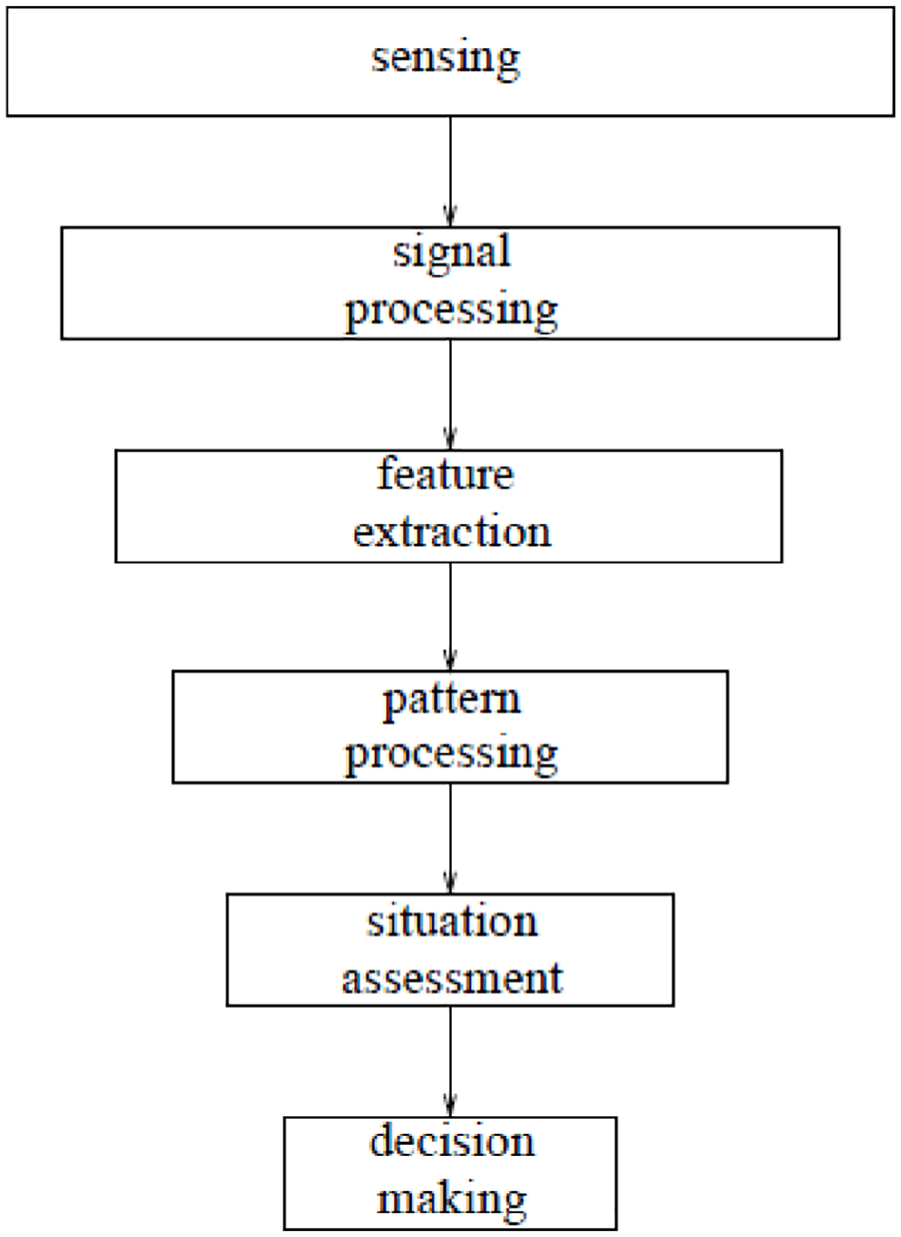
Waterfall model for SHM. 14
Pattern processing is typically carried out on a set of statistical features in order to infer meaningful correlations between signals and responses. A learning method is required, and this method can be supervised or unsupervised learning. Farrar and Worden
15
describe that if
training data comes from multiple classes and the labels for the data are known, the problem is one of supervised learning. If the training data do not have class labels, one can only attempt to learn intrinsic relationships within the data and this is called unsupervised learning.
In the absence of class labels, a one-class classifier can still be formed that defines only normal data; thus, anything not belonging to this class is fault data. This unsupervised learning technique that detects whether a new data point belongs to the normal class is known as novelty detection (it has also been referred to as anomaly or outlier detection). It is surprising to see that there has been such little discussion of unsupervised learning in the machining process monitoring literature. Several review papers from recent years, including those by Teti et al., 13 Liang et al., 3 O’Donnell et al. 16 and Bryne et al., 17 do not explore texts on unsupervised learning; however, they do highlight the issue that training data are expensive and presents a challenge to the production application. Some statistical methods have been applied in a few cases such as multivariate control charts as shown by Harris et al. 18 Furthermore, an unsupervised approach was presented by Dou et al. 19 that reconstructed monitoring signals from a sparse auto-encoder (SAE), then used the reconstruction error to indicate a change in state of the system due to tool wear.
Sick 20 reviews supervised and unsupervised neural networks for tool wear monitoring in turning. The author explains that since the tool wear measurements and cutting experiments are costly, unsupervised training presents an interesting approach. However, the author generalises in saying that ‘it is hard to believe that unsupervised paradigms can successfully be used in a monitoring system which is designed for practical applicability’. Research and industrial application in SHM 21 evidences the opposite. Practical application of unsupervised learning can be found in many scenarios and research fields, such as a good example from Coates et al. 22
Experimental approach and setup
The experiment discussed in this study captures multi-sensor data from a milling process. The intrusive nature of sensing in machining can be a limitation and so the sensing setup presented here has been designed to minimise any obstruction to the machining space. A base plate was manufactured with a cavity to contain all sensing hardware. In addition, two-directional microphones were installed in the machine tool, facing the cutting zone. The base plate is shown in Figure 2. It is important to note that while the base plate design has similarities to other lab-based sensing systems, the important feature of the design is that the cavity is relatively small and can be included in most fixturing scenarios. In a production setting the data acquisition unit would be included in the electrical cabinet of the machine.
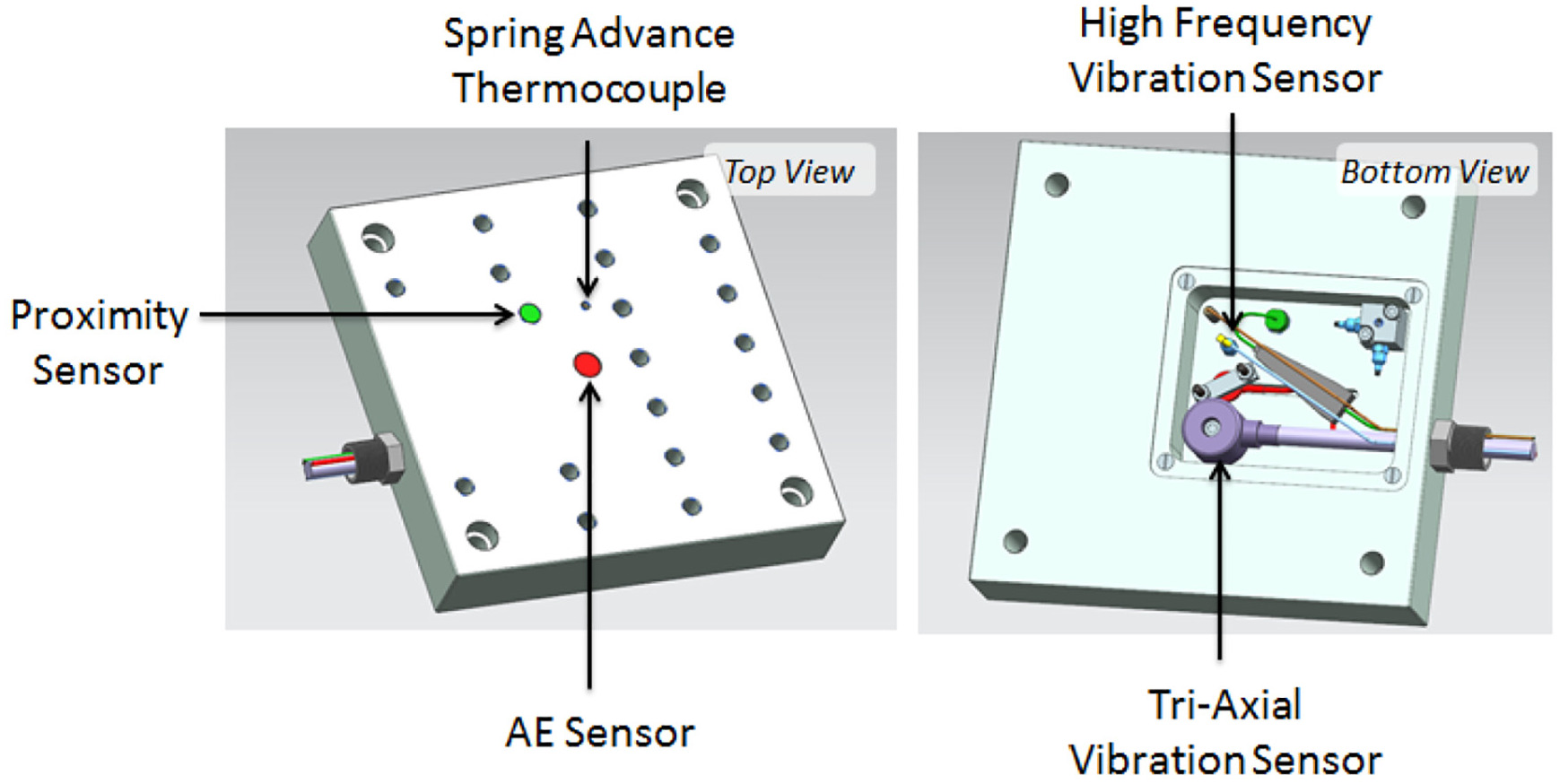
Sensor enclosure design.
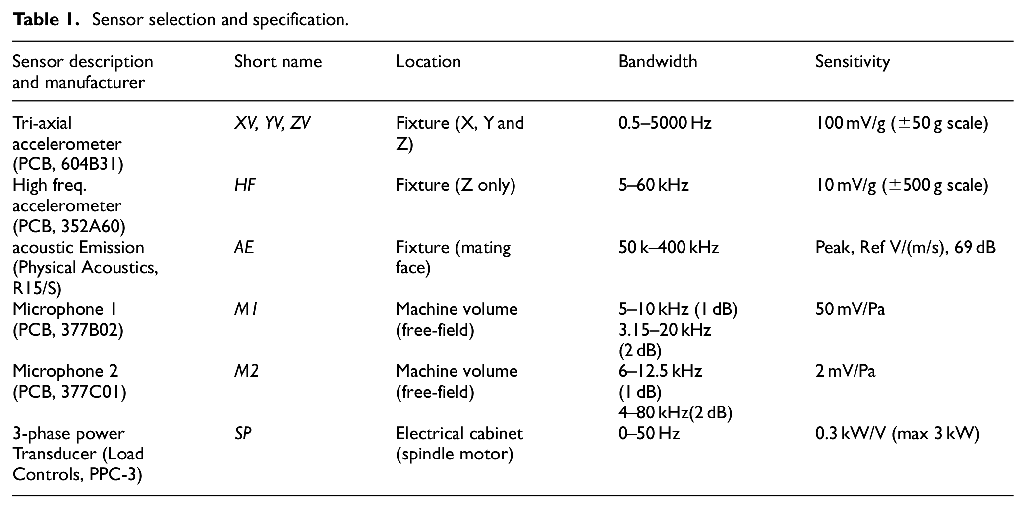
Choices of sensor types have been driven in part by those used in previous studies – it is common to include vibration, AE and spindle power within a sensing setup. In this case, a range of sensors are included to ensure a wide bandwidth of emissions are adequately sensed. A list of sensors used is provided in Table 1 and a summary of the sensor bandwidth is provided in Figure 3. (The proximity sensor and workpiece temperature sensor shown in the figure are excluded for this study.)
Sensor selection and specification.
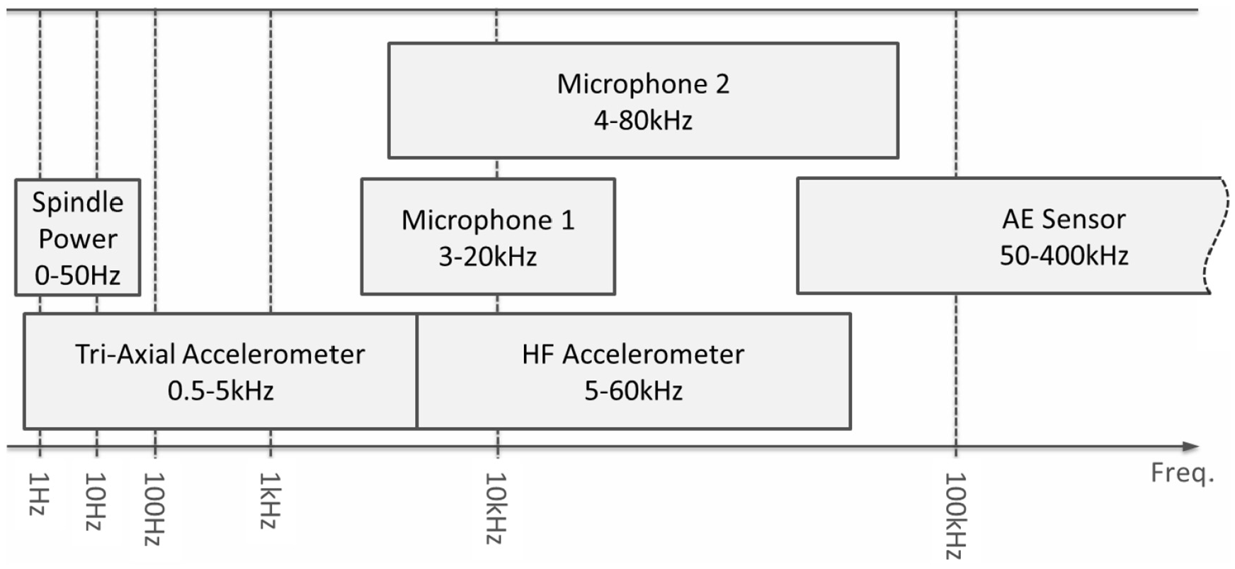
Sensor selection bandwidth.
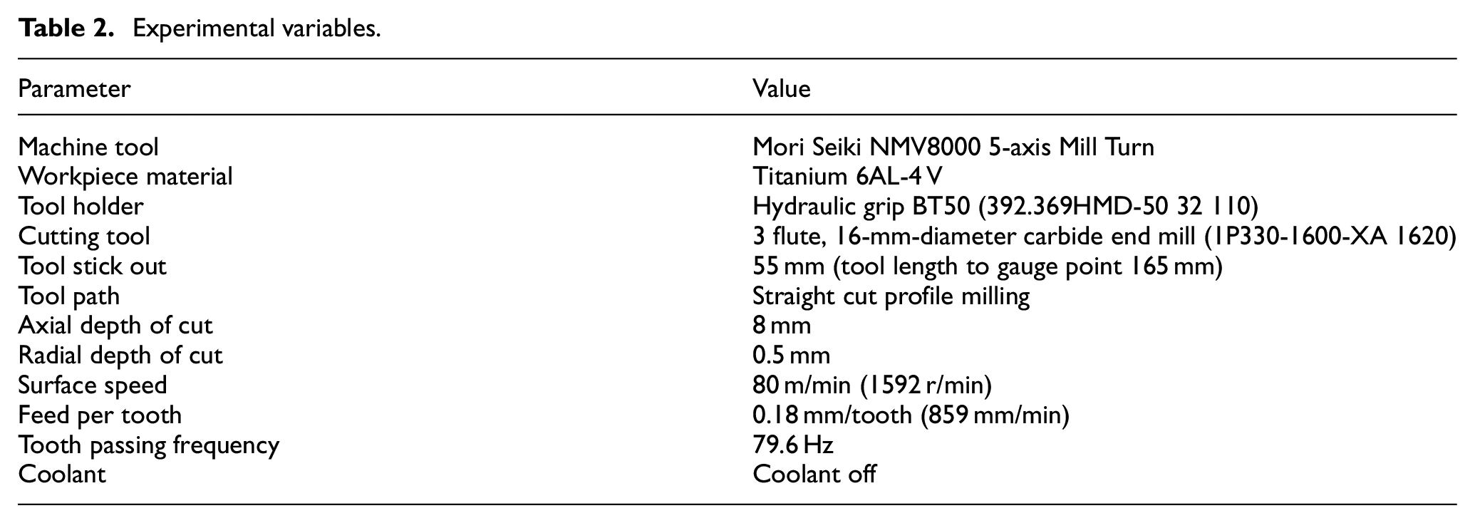
In this study, a three-axis finish profile milling process was performed on a titanium Ti-6Al-4 V work piece. The experimental data were obtained by running the new tool to a severely worn condition (defined by anything above 0.5 mm flank or notch wear width). The experimental variables are listed in Table 2 and a diagram of the experimental setup can be seen in Figure 4.
Experimental variables.
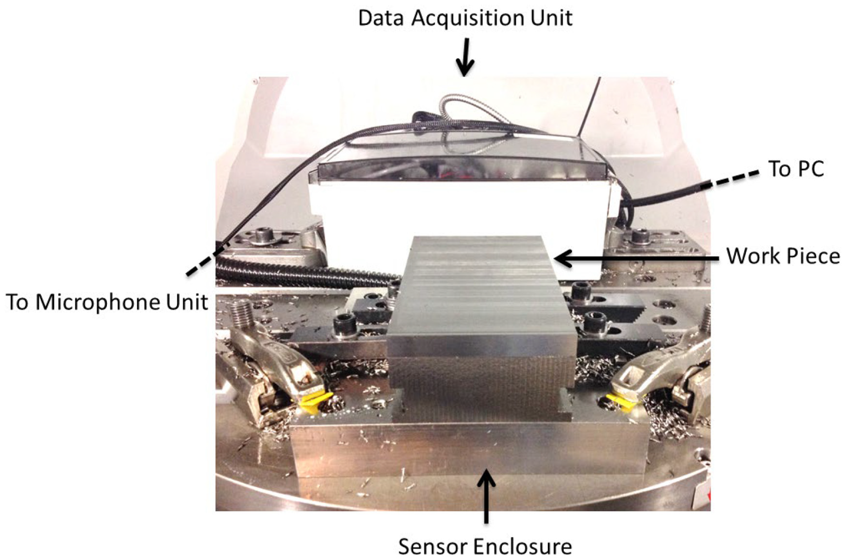
Experimental setup.
This article will focus on the numerical approach; however, more information on the tools condition and wear measurement data can be found in the work by McLeay. 23
Measured tool wear values are not required in this study, since the aim is to avoid the need for response data, allowing unsupervised learning technology to be applied. A judgement on what part of the experience can be considered normal must still be made, so that in the experiment one can collect a data set that, with reasonable confidence, can be used to define normal condition. Since it is reasonable to assume that a new tool will perform in a normal condition for a certain amount of time (in relation to tool wear), the machine operator has indicated at what point in the experiment they believe the tool should no longer be considered ‘normal’. From this observation, a normal condition data set can be defined.
Referring back to the sensors listed in Table 1, all eight channels of raw sensor data were captured using a ‘compact DAq’ data acquisition device available from National Instruments. The raw data were captured through LabView software using sampling rates of 100 kS/s, other than AE, which was sampled at 1 MS/s. Each cut taken was 9.2 s in duration and tools were run for approximately 60 min in the cut. Matlab was then used for all further computation, which is covered in more detail in the following section.
Results and analysis
The numerical analysis presented here essentially aims to reduce 8 waveform data sets into a simple classification of normal or faulty. A common challenge in implementing monitoring systems is the difficulty for them to generalise and perform in different settings. This is both due to a large number of different possible faults and the complexity and often subjectivity in deciding when a process can continue (normal) or must be stopped (faulty).
In this study, the change of the process from normal to faulty is simulated by progressive wear of the tool as time in cut increases. The point at which the process is classed as faulty is not unique to this scenario since it is based on a statistical measure of novelty.
The reader should note that this article provides plots of just some of the data captured in order to visualise the numerical approach. Of the eight raw sensor streams analysed, 151 time and frequency domain statistical features have been extracted. Some examples are shown in Figure 5 for frequency domain features from the Z-axis vibration signal. Two further time-domain signal features can also be seen in Figure 6.
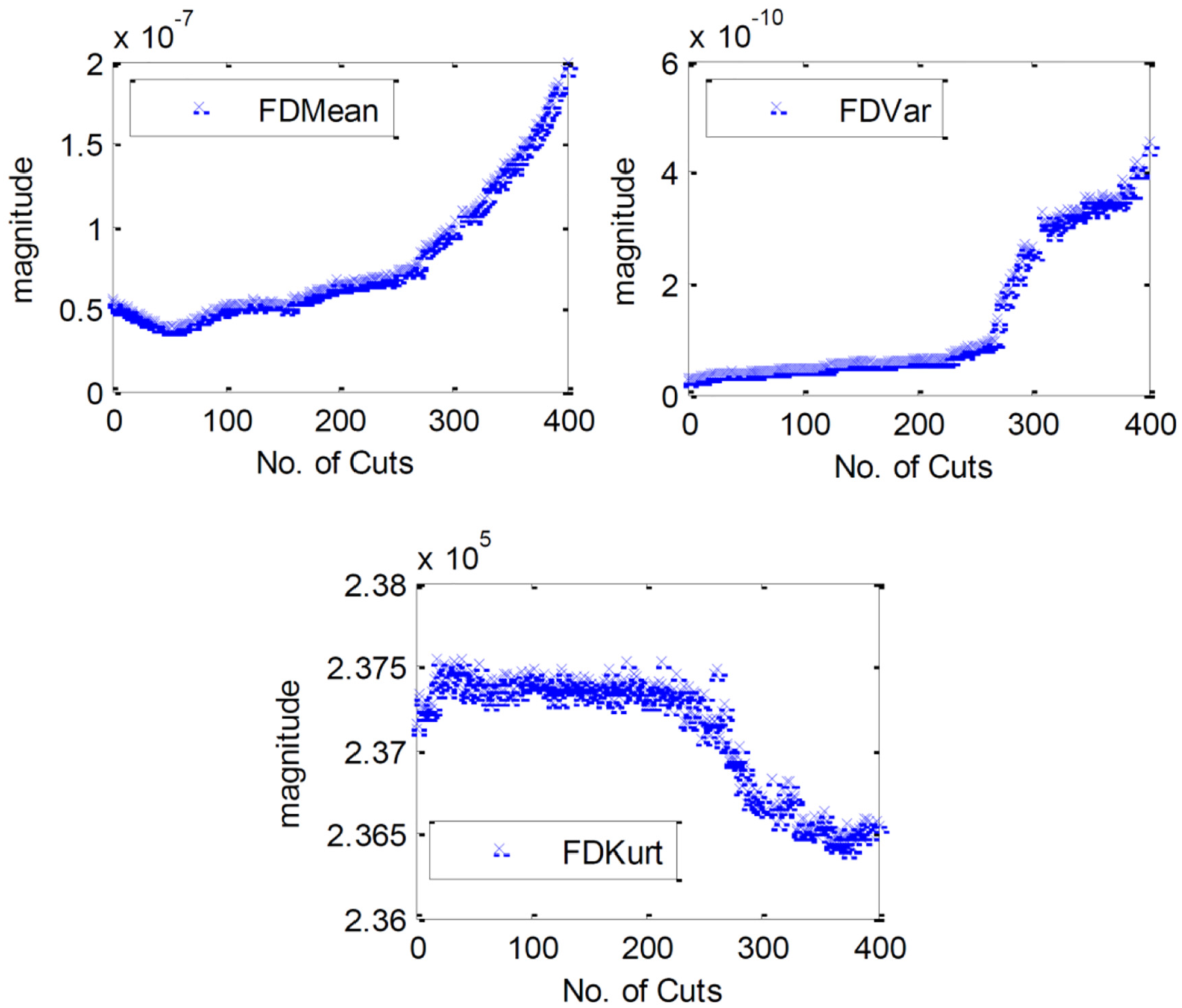
Frequency domain features for the Z-axis vibration signal. Features are the mean, variance and kurtosis of the power spectrum as indicated by graph legends.
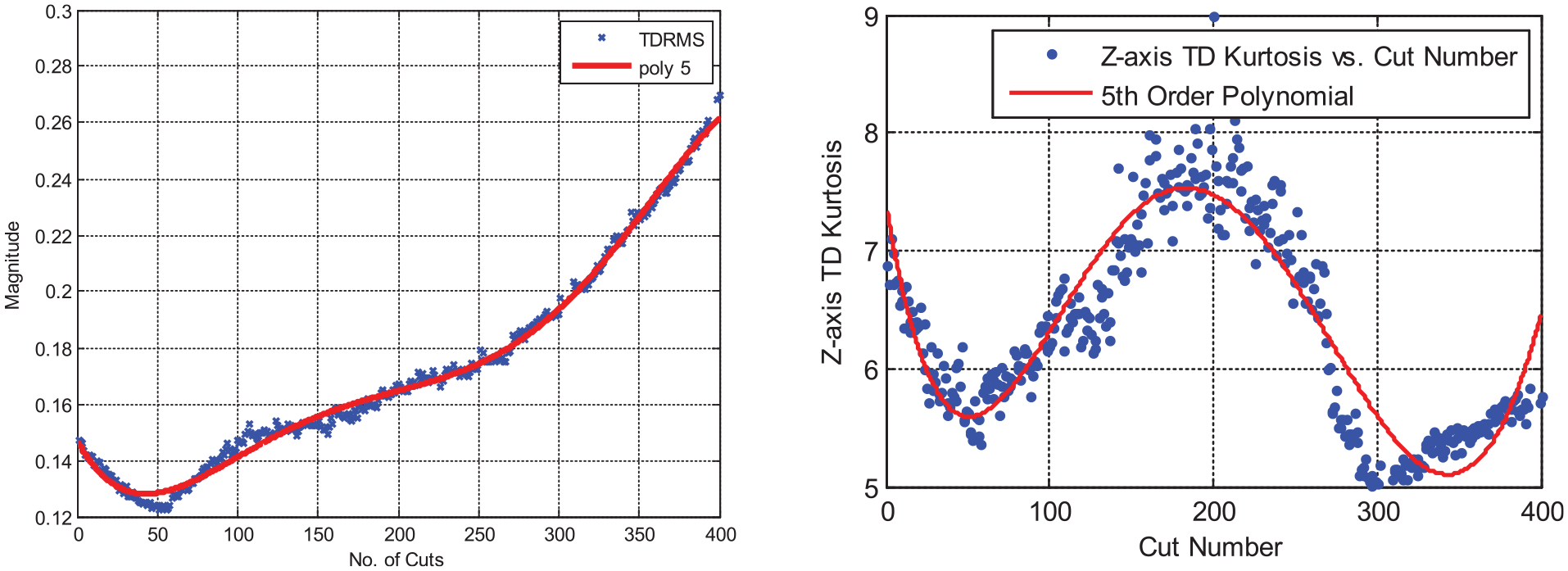
Polynomial fit example for two of the extracted features – a fifth-order model fits the RMS of Z-axis vibration data with an R-squared of 0.99. The same order model fits the Kurtosis with an R-squared of 0.85.
Methodologies for feature extraction have been regularly applied in the previous literature and so will not be expanded on in detail here. A more extensive review of the signals and extracted features gathered from this experiment can be found in the work by McLeay. 23
Feature selection is applied to reduce the data further by selecting only the features with the most useful information towards the objective. A filter method for feature selection has been chosen since this can provide greater computational efficiency when compared to wrapper methods. The following analysis first describes the method for ranking of all features based on evidence that they correlate with the condition of the process.
To rank each feature’s ability to trend the changing condition of the process, polynomial curves are fit to each feature. A monotonic model has intentionally been avoided, since in some cases cutting conditions can improve as cutting edges undergo a small amount of wear, for example. A model estimate data set is extracted using a random selection of the data points. The remaining data points are then compared to the resultant model and the R-squared goodness of fit value is used as the measure of fit, and therefore, as the measure of information content in that feature. The model order is identified by increasing order incrementally until minimal improvement in fit is observed.
The model fit gives a ranking of each of the 151 available features. When selecting the optimum subset of these features, it is also desirable to minimise redundancy within the subset and not keep multiple features that contain the same information. A method of finding a suitable feature subset was presented by Cho et al. 24 where subsets were ranked by the ‘Merit’ formula. The formula for the Merit of any feature subset is given by
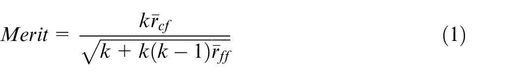
where k is the number of features in the subset,
As there are many different combinations of subsets, a sequential feature subset selection method was employed. While not an optimal method of subset selection, it is an efficient one, and is therefore scalable to larger data sets. Starting with a subset size of 1, each feature is added to the subset individually, ranked using the Merit score, and the highest-ranking feature is retained. The process repeats itself until a maximum Merit score is found. The sequential feature selection method can also occur in reverse, beginning with all features and removing the feature that has the greatest decrease in the Merit score. The results of the forward and reverse feature selection are shown in Figure 7.
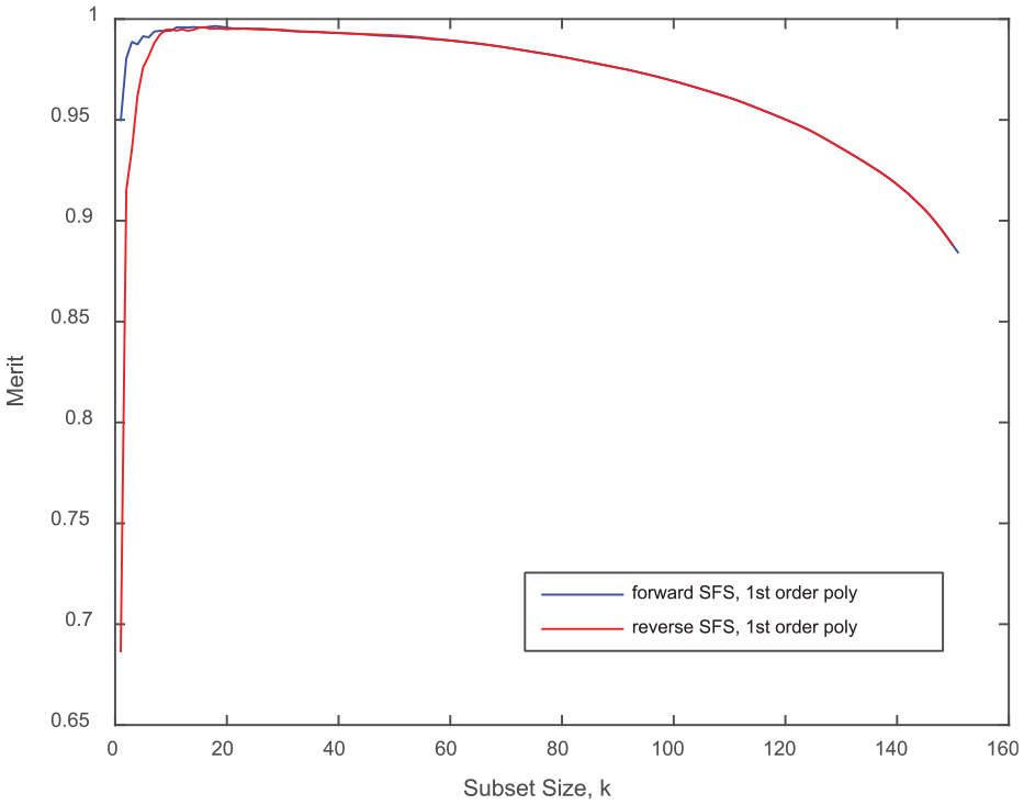
Sequential feature selection results to identify the optimum subset.
The optimum feature subset identified is shown in Table 3. It can be seen that a full range of features has been ranked in the optimum subset, both time and frequency domain. Only the second microphone failed to have any features in the optimum set. With this selection, the final analysis is now able to be conducted on a much reduced data set with 13 dimensions.
Optimum feature subset using sequential feature selection and Merit.
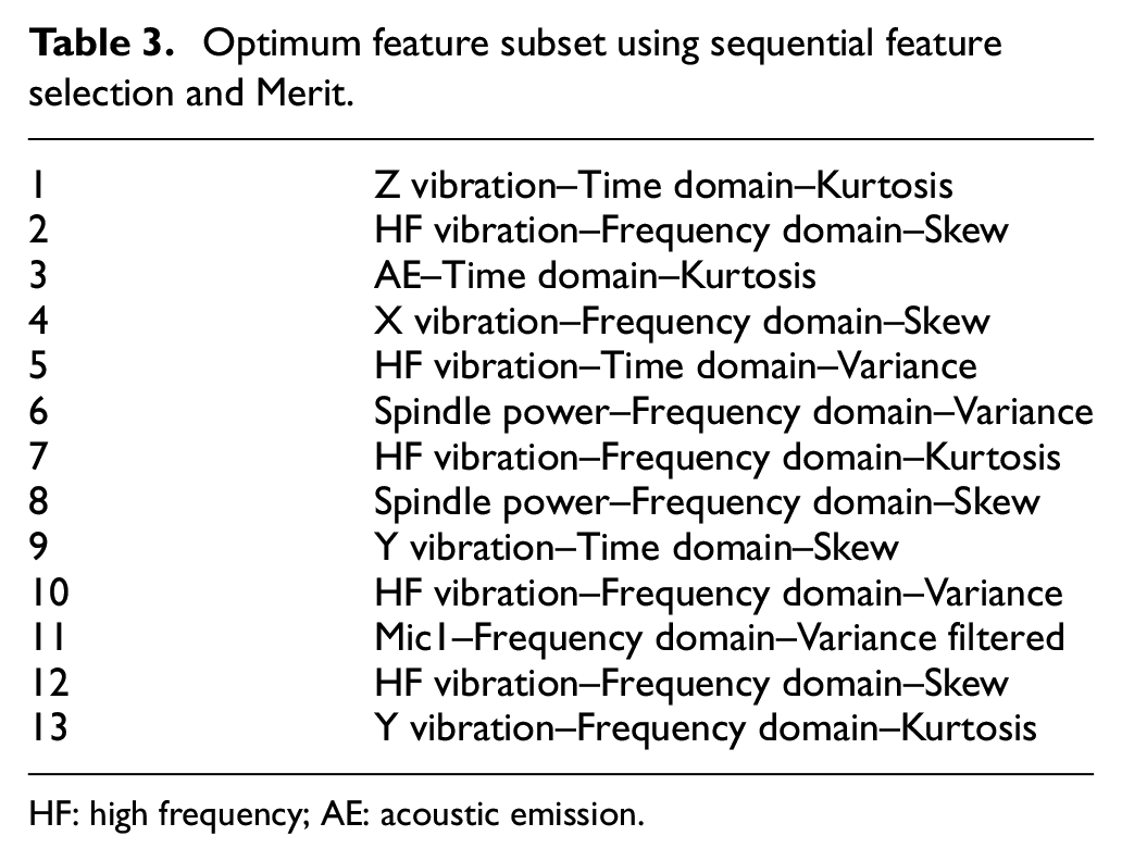
HF: high frequency; AE: acoustic emission
Novelty detection
Now that a feature subset has been identified, a method to detect when the process is in the normal state, and when it has a fault. A measure of how dissimilar a sample of feature data is to other samples provides the basis of novelty detection. Such a measure is referred to as discordancy and further reading is available from Barnett and Lewis. 25 A novelty is a sample which has a large discordancy in comparison with other samples in a data set. A novelty threshold then sets the magnitude above which the discordancy is a novelty.
For a process fault such as tool wear, a new tool begins without wear and therefore is operating under ‘normal’ conditions. Therefore, we can say that for cuts
To demonstrate the proposed method of fault detection, an estimate of the end of the tool’s life in Experiment 1 is made using expert opinion. The machine operator observed no issue with the cutting conditions until 41 min in cut (cut 266), at which point evidence of tool wear and deteriorated surface finish could be visually observed. All cuts through to 41 min will, therefore, define the normal condition and all subsequent cuts will define the faulty condition.
The Mahalanobis squared-distance can be used to determine the degree of discordancy of a sample from the normal condition sample set. The Mahalanobis squared-distance is a measure of the distance between a sample and the centre of a Gaussian distribution weighted according to covariance, calculated from the following equation

where
Figure 8 presents a scatter plot of the selected feature subset. The normal and faulty data are derived by expert opinion as explained earlier. Principal component analysis (PCA) has been used solely to aid the presentation of the data in two dimensions (it is otherwise not part of the analysis for this article). The plot presents the data using the two most significant components. The colour bar shows the log of the Mahalanobis squared-distance from the normal condition data (calculated using all 13 dimensions of the feature set). The trajectory of the data over time is illustrated by the arrows in the plot, also noting five different transition points where the trajectory changes. Each of these points is described briefly below:
After 6 min (cut 39), the trajectory of the data changes;
After 24.4 min (cut 159), a single cut is outlying and marks another change in the trajectory of the data;
At approximately 41 min (cut 266), the process makes a jump away from the previous cluster of data. This coincides with the same cut that the machine operator has decided that the process is no longer acceptable;
At approximately 53 min (cut 345), again the trajectory of the data changes, and finally the testing ends at 61 min (cut 397) in the cut at point (5).
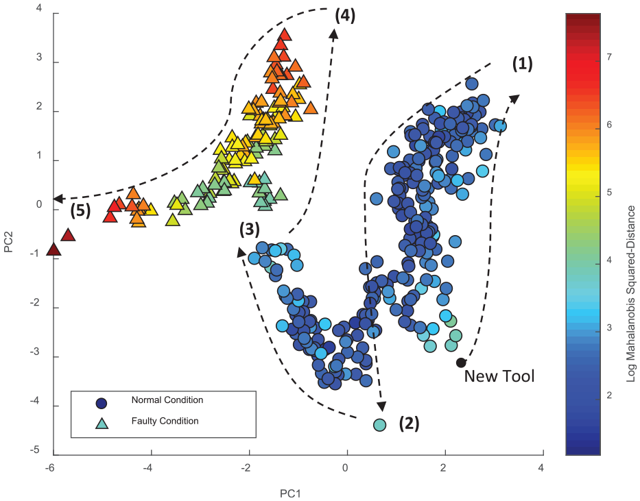
Scatter plot of Log of Mahalanobis Squared-Distance with the trajectory of data illustrated.
Figure 9 presents the same scatter plot data now labelled as clusters according to the grouping listed above. Here one can see some more structure in the data that precedes the faulty condition of the process.
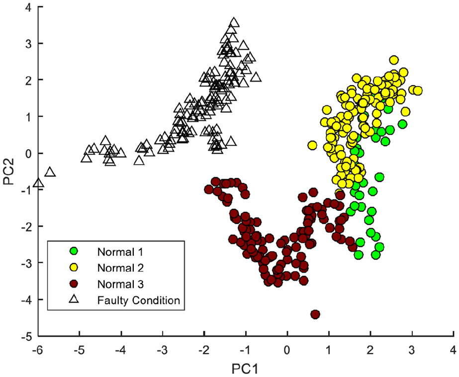
Scatter plot showing the clusters of data observed by comparing with the time in cut (Normal 1 = cut 1–38, Normal 2 = cut 39–158, Normal 3 = cut 159–265, Faulty Condition = cut 266–396).
Figure 8 presents several areas that warrant further discussion, and indeed future research opportunities. First, a key aspect of novelty detection is the definition of the normal condition. In this study, the normal condition has been defined by expert opinion on when the process was operating as normal, but the sensitivity of the system to this decision would need to be considered.
In Figure 8, it is clear that the normal condition data do not take a Gaussian distribution. Instead, the data set is convex, whereas the separate clusters shown in Figure 9 are individually more Gaussian in appearance. This suggests that the tool has multiple different states while still considered to operate in a normal condition. Further research and experimentation would be required to understand whether these states are consistent with specific wear states of the tool, and of course whether the behaviour is reproduced as the process is subject to environmental or operational changes.
Selecting a novelty threshold
As mentioned previously, often there is complexity and subjectivity in judging whether any machining process should continue or should be stopped; therefore, a generalised statistical approach to determine this threshold is appealing. A novelty threshold can be defined using the Monte Carlo method applied in the works by Cross 26 and Farrar and Worden. 15
Figure 10 shows the Mahalanobis squared-distance against the number of cuts. A 95th percentile novelty threshold is also included. The process exceeds the novelty threshold at 43.4 min in cut (cut 283). Recall from earlier that the expert opinion was that the process was behaving as normal up until 41 min (cut 266).
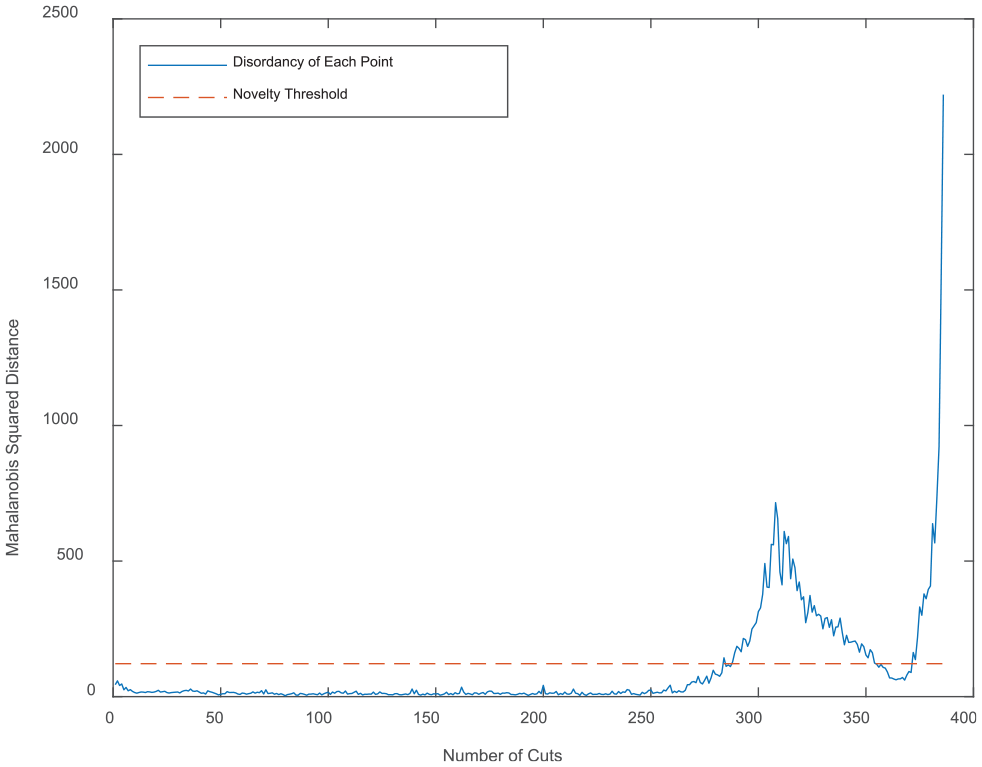
Mahalanobis squared-distance against number of cuts, including 95th percentile novelty threshold.
Generalisation of the approach
A single type of machining process was used to demonstrate the technique in this study, although it is proposed that the methodology is, by design, able to generalise to other machining processes. Indeed, the statistical technique can be generalised to many damage detection problems.
The statistical approach makes two assumptions for such generalisation. First, the normal condition of the process can be obtained easily, with reasonable confidence the data points represent normality, and that the data are Gaussian. Second, the sensor feature data set contains information about the relevant process fault(s) to a sufficient degree that the deviation is statistically significant. Other than these points, the method is agnostic to the type of process being monitored.
A flexible and low-cost approach is used to define the normal condition – it is required that, without additional measurements to be taken, a data set can be captured from the target process that is, with reasonable confidence, considered to be normal. This involves capturing a set of data when the process is operating normally, and so it is a method that can be adopted in the most demanding production environments where system configuration and model training is previously prohibitive (e.g. where the tool wear data must be measured, or faults must be simulated or labelled).
Conclusion
A novel method for observing changing conditions of a machining process and determining when the process can be classed as faulty has been demonstrated using unsupervised learning methods. A sensor system has been designed and built that is minimally intrusive to the cutting process but still acquires informative signals that describe the cutting conditions. The information content of sensor signal features has been successfully selected using a polynomial model fitting method. A feature set was found by first using a heuristic to score the information content of a subset, and then sequential feature selection for finding the optimum subset. Finally, using novelty detection, the Mahalanobis squared-distance has been used to determine the discordancy of data points from a user-defined normal condition data set. Fault conditions can be observed as clusters in a PCA plot. The point at which the process becomes defined using a generalised statistical approach–by calculating a principled novelty threshold using a Monte Carlo method that has been previously demonstrated in other research fields.
Footnotes
Declaration of conflicting interests
The author(s) declared no potential conflicts of interest with respect to the research, authorship, and/or publication of this article.
Funding
The author(s) received no financial support for the research, authorship, and/or publication of this article.