Sage Journals: Discover world-class research

Abstract

Bearings are the most widely used mechanical parts in rotating machinery under high load and high rotational speeds. Operating continuously under such harsh conditions, wear and failure are imminent. Developing defects give rise to even-higher vibration and temperature levels. In general, mechanical defects in a machine cause high vibration levels. Therefore, bearing fault identification and early detection enables the maintenance team to repair the problem before it triggers catastrophic failure in the bearing. Machine downtime is thus avoided or minimized. This paper explores the use of Machine Learning (ML) integrated with decision-making techniques to predict possible bearing failures and improve the overall manufacturing operations by applying the correct maintenance actions at the right time. The accuracy of the Predictive Maintenance (PdM) module has been tested on real industrial production datasets. The paper proposes an effective PdM methodology using different ML algorithms to detect failures before they happen and reduce pump downtime. The performance of the tested ML algorithms is based on five performance indicators: accuracy, precision, F-score, recall, and an area under curve (AUC). Experimental results revealed that all tested ML algorithms are successful and effective. Furthermore, decision making with utility theory has been employed to exploit the probability of failures and thus help to perform the appropriate maintenance interventions. This provides a logical framework for decision-makers to identify the optimum action with the maximum expected benefit. As a case study, the model is applied on forwarding pumping stations belonging to the Sewerage Treatment Company (STC), one of the largest sewage stations in Qatar.

Keywords

Fault detection predictive maintenance machine learning binary classification utility theory sensor data

Introduction

Bearings are essential components of most rotary machines, failure of which contributes to a reduction in the performance of production lines and may eventually lead to the breakdown of these machines.¹ In bearings, most of the faults occur due to wear loss in their elements (i.e. inner race, outer race, and rolling parts) which in general, can dominantly be detected by mechanical noise, temperature, and vibration.² Therefore, the most frequently identified problems in bearings can be summarized as the following³:

Insufficient or excessive lubricant,

Poor installation of the bearings,

Small bearing clearance or heavy load,

High friction between lip and seal groove,

Improper lubricant type, and

Creep between the fitting surfaces.

However, the unexpected failure of the bearings can be very expensive due to many factors such as loss of production, cost of replacement, and significant damage to other parts of rotating machinery.^4–6 Hence, early detection techniques by continuous condition monitoring^7–10 have appeared as promising means to avoid catastrophic component failure of the machines by sensing, measuring, and recording the physical variables that collected from the sensor-mediated components^11,12 and thereby these data are functionalized according to particular operating conditions. More specifically, when the operating conditions reach a certain critical level, alerting signals are displayed by developed models to apply predictive maintenance (PdM).^13,14 Predictive maintenance primarily involves expecting a breakdown of the system to be maintained by detecting early signs of failure to make maintenance jobs more proactive.¹⁵ PdM aims at predicting failure time of a system based on experience, physical laws, and machine learning techniques to replace the faulty components before failure, and as the result minimizing downtime of the systems, reducing the maintenance costs, and improving quality of product.¹⁶

For PdM, a variety of technologies can be used as parts of a comprehensive program including monitoring and diagnostic techniques. These techniques include vibration monitoring,^5,17–19 acoustic emission,^20,21 thermographic inspection,²² oil analysis,^23,24 Radiographic inspection,²⁵ shock pulse,²⁶ ultrasonic leak detectors,²⁷ performance testing, wear and dimensional measurements,²⁸ signature analysis,²⁹ and time and frequency domain.^30,31 Among the above techniques, vibration analysis has attracted a great deal of attention as time domain and time-frequency domain for tracking machinery operating conditions which in turn successfully diagnoses the defects and increases the machinery life. In this regard, vibration signals are firstly gathered and processed using vibration analyzers equipped with sensors in the time domain. These signals are then converted into the frequency domain using Fast Fourier Transform (FFT) to extract the frequency signature. The information obtained from the vibration signals has significant advantages in terms of predicting catastrophic failures.³²

The networking of physical devices and computers which assist in collecting and sharing the data is called the Internet of Things (IoT). These devices have formed a gateway to connect to machines and its subcomponents to not only collect the process data and its parameters but also to collect the physical health aspects of the machine such as vibration, pressure, temperature, acoustics, viscosity, flow rate, etc.³³ This information is widely used for early fault detection and identification, health assessment of the machine, and predicting the future state of the machine. Some of this is made possible owing to machine learning (ML) algorithms available through different learning domains.³⁴ IoT has also been versioned for the application in maintenance, particularly PdM. As reported in references,^15,35 the advances in information, communication, and computer technologies, such as IoT and Radio-Frequency Identification RFID, have enabled PdM to be conducted more efficiently with enhanced data collected in a time-efficient manner.

The machine learning model is a mathematical model that generates predictions by finding patterns in the data. ML helps in solving many problems in big data, vision, speech recognition, and robotics.^36,37 It can be classified into three types: supervised-, unsupervised-, and reinforced learning. Unlike the first type in which the predictors and response variables are known for building the model, in the second type only observations are known. However, in reinforced learning, the agent learns actions and consequences by interacting with the environment.^34,38,39 Supervised ML aims at building a predictive model of the classification of class labels to determine the predictor features. The resulting classifier is then used to assign class labels to the testing dataset where the values of the predictor features are known, but the value of the class label is unknown. As far as this work is concerned, the authors have chosen supervised ML as a prediction model in terms of analyzing the collected data.

Related work

Tian et al.⁴⁰ presented a fault detection method of oil pump based on Support Vector Machines (SVM) which its parameters were optimized by genetic algorithm. Associating the ability of strong self-learning with the generalization of SVM, the detection method was truly shown to diagnose the fault in oil pumps by learning the fault information. The real detection results showed that the proposed method was feasible and effective. Samantaray⁴¹ presented a new technique for high impedance fault (HIF) detection in a power distribution network using ensemble decision trees (random forest RF). The process included two stages: the first was estimating the amplitude and phase of harmonic contents in the HIF current signal whereas, in the second stage, the random forest was trained with the amplitude and phase information of the HIF current signal. The results indicate that the proposed method can reliably detect more than 99% HIF in a large power distribution network. Li et al.⁴² showed that application of analytical approaches (including correlation analysis, causal analysis, time series analysis, and ML techniques) against both historical and real-time data such as failure data, maintenance action data, inspection schedule data, train type data, and weather data led to failure predicting in the future, thus avoiding service interruptions and increasing network velocity. Kroll et al.⁴³ presented an approach that used timed-hybrid automata of the machine’s normal behavior for PdM of industrial plants. They have demonstrated that this method has an advantage over a traditional, static limit testing. This advantage is a model of the whole continuous dynamics, which reduces it to separately modeled state vectors. This, in turn, allowed effective anomaly detection by implementing a combined data acquisition and anomaly detection approach, and presented outlook for other applications, such as PdM planning.

Cline et al.⁴⁴ demonstrated the potential of ML techniques on enhancing the operations of an Oil and Gas equipment service department. Analyzing significant data sets of individual machine performance resulted in major improvements in the customer’s ability to identify risky assets up to 1 year in advance. Paolanti⁴⁵ described the ML architecture for PdM on the base of the Random Forest approach. The system was tested on a real industry example by developing the data collection and data system analysis, applying the ML approach, and comparing it to the simulation tool analysis. Data collection has been done using various sensors, machine programmable logic controllers (PLCs), and communication protocols before being available to Data Analysis Tool on the Azure Cloud architecture. Preliminary results show a proper behavior of the approach to predicting different machine states with high accuracy. Amruthnath and Gupta³⁴ who have chosen a simple vibration data collected from an exhaust fan and have fit different unsupervised learning algorithms such as Principal component analysis (PCA), T² statistic, Hierarchical clustering, K-Means, and Fuzzy C-Means to test its accuracy, performance, and robustness, have eventually proposed a methodology to benchmark different algorithms and choosing the final model. In their study, the T² statistic provided more accurate results compared to the Gaussian mixture model (GMM) method. However, Clustering methodology is undoubtedly a better tool in detecting different levels of faults where T² statistic would be challenging after certain levels. Strictly speaking, when the cost of machine maintenance is expensive, clustering would be a flexible option where machine health can be monitored continuously until a critical level is reached.

Recently, Allah Bukhsh et al.⁴⁶ employed the ML techniques for the development of PdM models based on decision tree (DT), random forest (RF), and gradient boosted tree (GBT) by using existing data from a railway agency. For the prediction of maintenance need, the GBT model performed most optimally as compared to other methods with 86% accuracy. For maintenance activity type and trigger’s status prediction, the RF model attains an accuracy of 70% and 79% on the held-out test set respectively. They proposed that by collecting more data, specifically for minority classes, the predictive performance of the models can even be further improved. Gutschi et al.⁴⁷ presented a data-driven approach for estimating the machine breakdown probability during a specified time interval in the future. The authors described applied data-mining, feature-extraction, and ML methods and concluded that machine failures can be reliably predicted up to 168 h in advance. Xayyasith et al.⁴⁸ presented the ML application for PdM of a water cooling system in Nam Ngum-1 (NNG-1) hydropower plant located by using the Classification Learner Application of train model. A 22 classifier types were organized in six major comparable classification algorithms (including Decision Trees, Discriminant Analysis, Support Vector Machines (SVM), Logistic Regression, k-Nearest Neighbors (KNN), and Ensemble Classification), it was shown that the SVM and Decision Trees are better at predicting faults as compared to the other algorithms used in this study.

In the last related work, Nam et al.⁴⁹ have applied a data-driven approach to develop a health monitoring and diagnosis framework for a fused deposition modeling process based on a machine learning algorithm. For the data-driven approach, three accelerometers, an acoustic emission sensor, and three thermocouples are installed, and associated data are collected from those sensors and processed to obtain root mean square values. Among various root mean square values, those of acceleration data from the frame were most effective for diagnosing health states of the fused deposition modeling process with the non-linear support vector machine-based model.

The current work which is concerned with the fault detection in bearings components of the forwarding pump stations helps the production managers in planning the maintenance activities, that is technicians and spare part availability. The supervised ML method has been applied in this study where the data fed (mainly temperature and vibration) belong to the labeled type. In this respect, a comparison among four different types of classifiers: decision trees, random forest, and gradient boosted trees as well as support vector machine. This comparison was achieved by utilizing python programming language to investigate which type provides the highest detection accuracy. Since the binary classification output of the applied ML algorithms can generate the pseudo probability of an observation belongs to a class the authors choose to use the utility theory to exploit the probability of failures and thus help to perform correct maintenance actions.

Research methodology

Figure 1 summarizes the research methodology which is based on an integration of an online fault detection algorithm with the decision theory for PdM. As the figure indicates, historical data are used for the offline model training, whereas online data are observed from instantaneous sensor measurement for predicting the process state. The utility theory is finally used for scheduling PdM.

Figure 1.

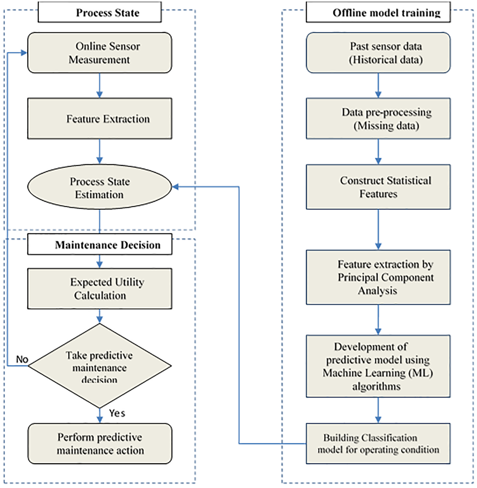
The flow chart of the proposed method for bearing fault prediction model.

The first stage to build the prediction model depends on data acquisition, a process of collecting and storing useful data from the target system to monitor the condition and diagnose the faults. The input for the data acquisition process is vibration signals and temperature readings. These signals are extracted to reduce the dimension of feature space where the reduced features are fed to several types of ML algorithms to classify the operating conditions. Performance comparison among the tested ML algorithms is performed to select the one with the most accurate bearings faults prediction. The selected model is then used to process state estimation for online sensor data measurements after feature extraction. Besides, we utilize utility theory coupled with the probability scores resulted from ML to guide decision-makers on when to implement the maintenance activities in an efficient and cost-effective manner. Therefore, our decision model provides a well-defined framework for the selection of the correct maintenance action. The following sections explain more details of the study main stages.

Offline model training

Several statistical features were extracted to train the ML models that, in turn, generate the final fault predictions. Seven descriptive statistical features for each sensor signal were constructed from the selected dataset of the bearing component: they are mean, skewness, kurtosis, maximum and minimum values representing the upper and lower ends of our data. The standard deviation (SD) and root mean square (RMS) was also included.⁶ These statistical features are calculated for each selected attribute (i.e. temperature and vibration) that gained from six different sensors. Among those features, the RMS values are considered the most effective to distinguish the differences between healthy and faulty states.⁴⁹

The binary classification is viably used for PdM, being able to estimate whether the equipment will fail over a future period of time. To use the binary classification, it is necessary to identify two types of classes, represented by zero and one. Each class is a record of a unit of time for an asset that conceptually describes the operating conditions, taking into consideration the technical data of the pump design as well as its specifications.

In the context of the PdM binary classification, the class “1” denotes the faults while the “0” class stands on the normal operation condition. This classification aims to find a model that identifies the condition of which each bearing may fail or work normally in the future. In the present work two different operating conditions have been considered, the first condition was labeled as normal, where no faults were present in the bearings. Whereas the second one is known as fault indication condition (announced when the operating conditions of the bearings, that is temperature or vibration, reach to or go over the critical limit value) are summarized in Table 1.

Table 1.

Selected attribute classification.

Description	Range	Critical limit	Model classification
Pump DE & NDE temperature	0–200°	80°	0: Normal operating condition <80°
			1: Fault indication when ≥80°
Pump DE & NDE vibration	0–10 mm/s	6 mm/s	0: Normal operating condition <6 mm/s
			1: Fault indication when ≥6 mm/s

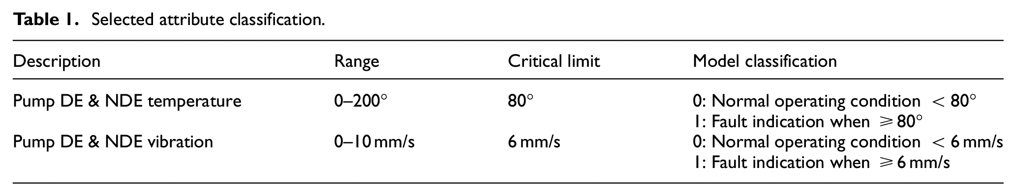
Thus, the ML approach applied to temperature and vibration data has mainly focused on finding the relations between normal and critical operation conditions to extract the most likely root causes for bearings faults determination.⁵⁰

Temperature measurements help in potential failure estimating which are related to the temperature change in the equipment such as excessive mechanical friction (faulty bearings, inadequate lubrication, fouling in a heat exchanger, and poor electrical connections). While those of vibrations can indicate problems such as wear, imbalance, misalignment, and damage.⁵¹ These measurements contribute to determining the causes of the faults that occur in the bearings mainly due to either temperature and/or vibration. In accordance with the results that came from these observations, expert knowledge of maintainers as well as the maintenance manual of pumping machinery, the right maintenance action can be executed.

ML algorithms

Decision Tree (DT), Random Forest (RF), Gradient Boosting (GB), and Support Vector Machine (SVM) algorithms are used to find the best classifier for the data under study. A brief introduction about ML algorithms is given in the following.

Decision Trees (DT)

In respect of this, Sheng and Rovnyak⁵² and Kotsiantis et al.⁵³ have made an overview of decision trees in which the advantages of the DT in ML have been given. Therefore, the authors of the current paper have chosen the decision tree which is a well-known technique in providing the logic-based rule as well as those of classification by tracing down the nodes and branches in the tree. It, furthermore, turns out the decision tree model that gives good results and, hence, satisfies the accuracy requirement and generates simple logic rules that can be interpreted as straightforwardly by operators.

In respect of the proposed ML classification model, the binary classification (0,1) dependent-decision trees exhibit better tendency in terms of its performance and consequently, the decision/classification can be quickly calculated.⁵⁴

Random Forest (RF)

Random Forest, so-called ensemble decision trees, has been used in this work as a classifier algorithm for it gives better predictive results and also operates building multiple decision trees, providing faults detection with higher reliability and accuracy as compared with DT especially when the data are originally expanded.^55,56 Furtherly, RF is used to reduce the difference between the actual and predicted values like variance, bias, and noise which is not functionally included in RF.

Gradient Boosted (GB)

Gradient Boosted is an alternative ensemble learning technique that consecutively produces weak tree classifiers in a stage-wise fashion as other boosting algorithms do with a different base model. To implement the GB algorithm for a particular problem, we need to estimate the right size of tree and number of iterations (number of trees) that give the best prediction accuracy. Each iteration is an attempt to reduce the loss function such as cross-entropy or sum of squared errors which implies that the number of iterations should be large enough to minimize the error function.⁵⁷ Moreover, boosting algorithms are relatively simple to implement with different model designs.⁵⁸

Support Vector Machines (SVM)

Support Vector Machines (SVM) are probably the most popular approach which is primarily used in classification and regression of large sample size owing to their high classification accuracy, even for nonlinear problems and their availability of optimized algorithms for their computation.^39,59–61 In this context, the (SVMs) has received great attention in the last years in much research especially in the field of machine condition monitoring and diagnosis.⁶²

Decision-making theory

Aiming at determining the optimal strategy alternatives, decision making and utility theory have been comprehensively used in the design of manufacturing and production activities.⁶³ In our case study, there is a list of $d_{1}, d_{2} \dots d_{m}$ of decisions (such as taking, or not, the maintenance action) and $Ø_{1}, Ø_{2} . . . Ø_{n}$ of events (such as normal or critical conditions) with the uncertainty of probability $p (Ø_{j})$ of event $Ø_{j} (j = 1, 2 \dots n) .$

Among the possible decisions ( $d_{1}, d_{2} \dots d_{m}$ ), the optimal one is chosen to avoid the extra costs of incorrect maintenance that arise from unreal predictions which can be achieved by maximizing the expected utility function.⁶⁴ The utility of the consequence ( $u_{ij}$ ), in correspondence to a decision (i) on an event (j), is determined by a utility function. As for fault detection of bearings in the current work, there are two decisions, namely, $d_{1}$ : no maintenance action (continue working) and $d_{2}$ : perform maintenances action along with two events $Ø_{1}$ and $Ø_{2}$ which present normal and critical conditions, respectively. The two correct decisions are: (a) to do maintenance if it is a critical condition and (b) to continue operating pumps if the normal condition has a significant utility.

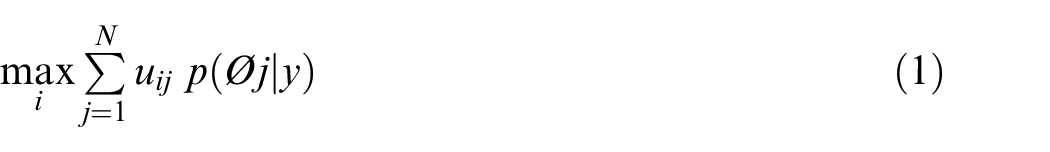
To compute the expected utilities for different decisions, formula (1) is considered for which the probabilities for each event $p (Ø_{j})$ shall be determined.⁶⁵ They can be initially estimated based on historical data. Thereafter, once the in-situ sensor data y is available, $p (Ø_{j})$ will be updated as $p (Ø_{j} | y)$ using ML algorithms. The optimal decision ( $d_{i}$ ) will thus be chosen based on maximal expected utility. This aims to obtain the optimum maintenance action which combines the reliability and availability for each possible action.⁶⁶

\max_{i} \sum_{j = 1}^{N} u_{i j} p (\emptyset j | y)

(1)

Case study

Sewerage Treatment Plant treats 245,000 m³ of wastewater on a daily basis which mainly used in irrigation and other non-potable purposes while the sludge from the treatment plant is used as a soil conditioner in the neighboring agricultural fields and as a source of green energy. For these purposes, vertical and single-stage forwarding pumps (TORISHIMA, Korea) are used. The technical specifications of these pumps are driver output: 840 kW, flow capacity: 4738 m³/h, total head: 47 m, speed: 730 rev/min, and frequency: 50 Hz. One of these many pumps is chosen from which the data used for applying ML algorithms, that is vibration and temperature, are collected at each minute, giving a total number of 130,956 data points which corresponds to a period of 3 months. As for the vibration, four accelerometers of sensitivity: 100 mV/g, sensitivity precision: ±5% at 25°C, and acceleration range: 0 to 80 peak were installed along vertical and horizontal directions to pick up the vibration (acceleration) signals created at Driving End (DE) & Non Driving End (NDE) Bearings. Likewise, there are two temperature sensors of type of Resistance Temperature Detectors (RTD)-PT100. These sensors are installed in the same directional mode with a measuring range between −50 and +180°C for DE & NDE Bearing. The schematic of the forwarding pump adopted in our study is depicted in Figure 2. Moreover, a photo of the pumping station and sensor types are shown in Figure 3.

Figure 2.

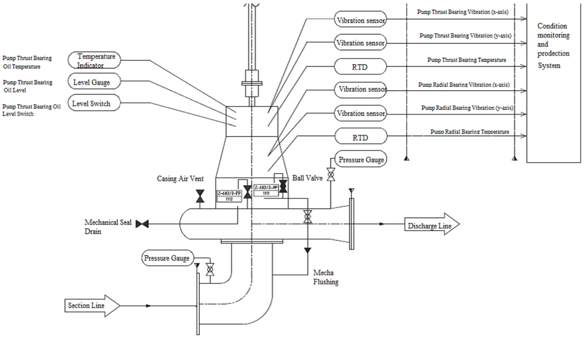
A schematic drawing of the forwarding pump and specific location of the sensors.

Figure 3.

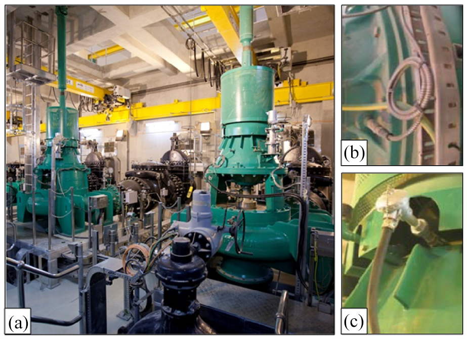
Photographs of the (a) PS70 pumping station, (b) vibration sensor, and (c) temperature sensor.

This paper presents a ML approach using data collected by IoT technology, specifically, by SKF@ptitude observer monitoring which is an expert diagnostics software usually used for pump monitoring system illustrated in Figure 4. It maximizes the rotating equipment performance (REP) via allowing more agile business, delivers greater output, reliability, and optimizes safety. A variety of sensors are installed along with the pumping system components used to measure the data needed as input to the ML. Furthermore, other relevant information is shown in user-friendly displays. Live data, updated every second, and long-term history can easily be displayed in many different formats. In the process overview window, live data and alarm indications are shown in descriptive pictures for pumps. SKF@ptitude observer gives direct measurements of bearing temperature and vibration. Besides, SKF@ptitude observer monitors bearing noise indicating defects that may eventually lead to bearing overheating problems. These recorded measurements are important to protect the machine where the observer gives an alarm if the recorded data exceeds a pre-specified threshold. Such a critical threshold is usually set depending on pump specification and manufacturing standard. For example, when the bearing temperature is greater than 120°, an alarm is triggered and immediately stopping the pump is required. In addition, when undesirable events occur, the software sends an alarm message to the maintenance management department which in turn evaluates the causes of this critical machine condition. However, due to their simplicity, they can only capture imminent overheating and bearing failure accurately. This does not provide enough lead time to perform PdM planning and resource optimization. This highlights the advantage of the current study which integrates the benefits of SKF@ptitude and the ML predictive power to detect the occurrence of abnormal conditions in advance.

Figure 4.

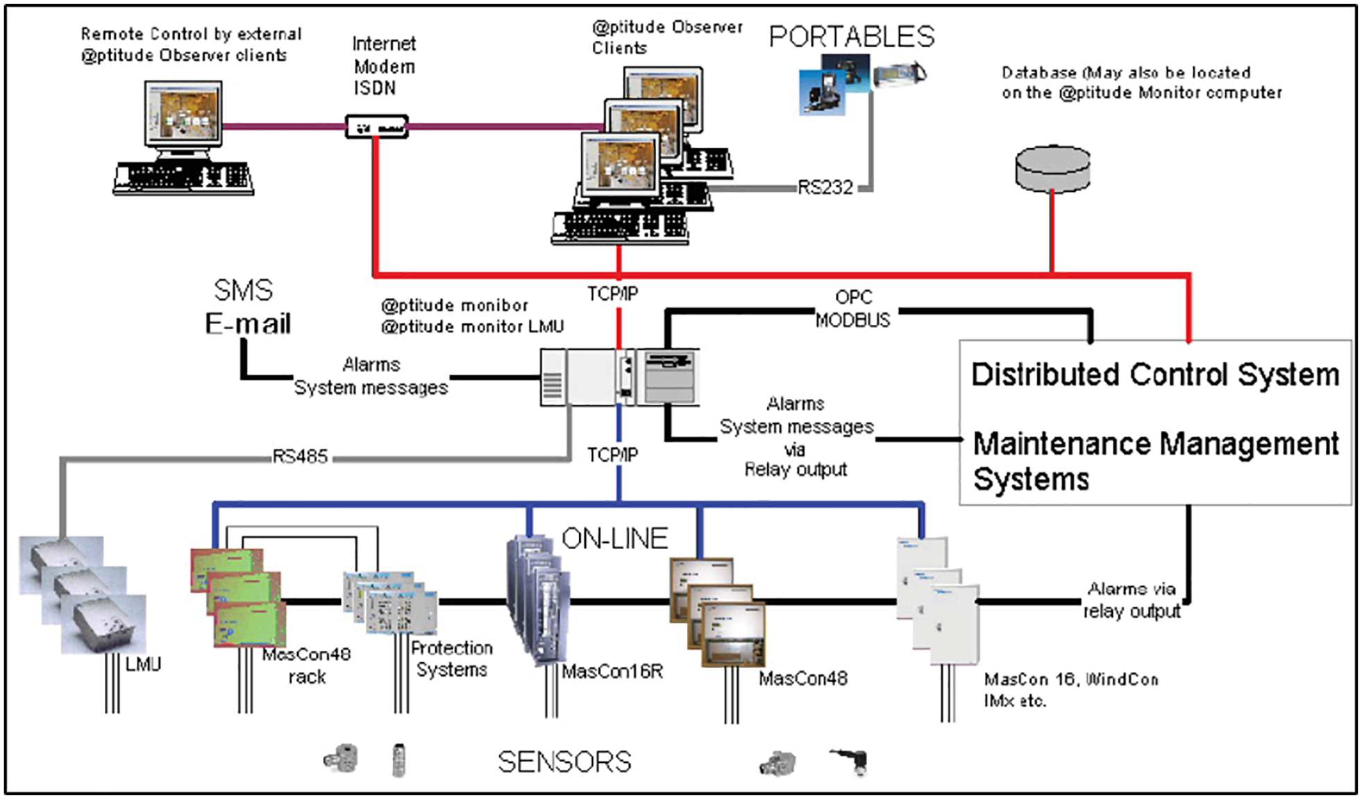
SKF@ptitude observer monitoring system.

Data collection and preprocess

Data collecting is the most important step in applying ML algorithms. As mentioned previously, this work is based on a real data-set collected from several types of sensors that monitor the pumping processes in the sewerage treatment company. The sensor data stream-in at an interval of 1 min, which is equivalent to 1440 rows of data per day, a description of the original data sets as a time series of accelerations and temperature shown in Figure 5. However, as reserved-dataset is not directly suitable to be used in creating a predicting model because it mostly contains noise and missing feature values. Therefore, the second step of data preparation and data preprocessing is applied before feeding it to the ML algorithm in order to convert the raw data into a clean data set and make them more suitable for further analysis.

Figure 5.

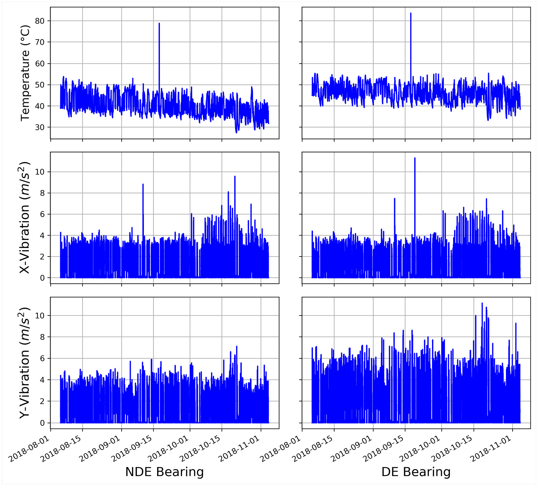
Features of the original data sets.

In this respect, feature extraction is used for data preprocessing that focuses on modifying the data for better fitting in a specific ML method. It also involves reducing the data by generating a smaller set of predictors that seek to capture a majority of the information in the original variables.³⁹ In this way, the original data are replaced by fewer variables providing a reasonable fidelity.

Dimension reduction

Principal component analysis method, the commonly used feature extraction technique,⁶⁷ seeks to find out the correlation nature among statistical features. It is also used to reduce the number of features by not only removing the ones among which the high correlations but also maximizing the variance over a set of instances.

Basing on this unique characteristic, PCA is finally used for the classification of variables and hence early identification of abnormalities in the data structure.⁶⁸ In respect of this explanation and according to the available data, a set of 42 statistical features for six attributes listed in Table 2 was reduced to a smaller set of seven uncorrelated final features corresponding to a 95% variance of the original data set.

Table 2.

Selected attributes for bearing prediction.

Type of sensor	Attribute
Accelerometer (vibration signal reading)	NDE Bearing (x-axis)
	NDE Bearing (y-axis)
	DE Bearing (x-axis)
	DE Bearing (y-axis)
RTD (temperature reading)	NDE Bearing
RTD (temperature reading)	DE Bearing

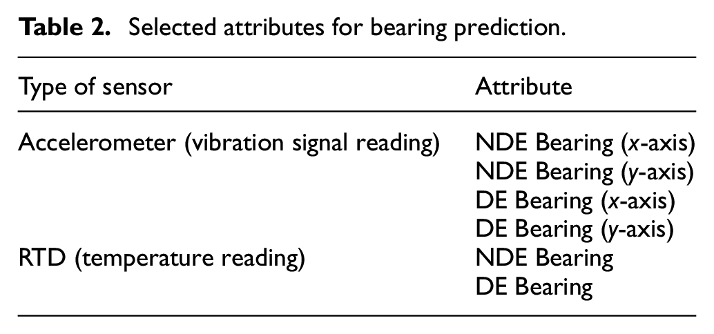
Figure 6 shows the change of the explained variance ratio of the 42 variables selected for PCA versus the principal component. It is can be seen that seven of these 42 variables have explained 95% of the variance. This means that the seven PCs subspace contains enough information about the variation of the original features which is sufficient to construct the model that can detect the faults in the bearing component

Figure 6.

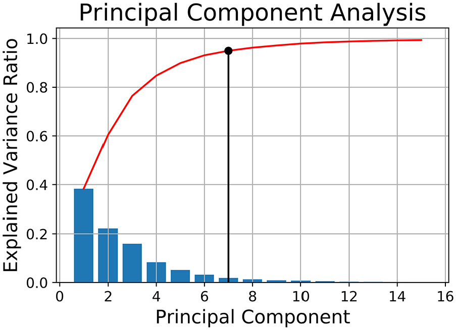
Principal component selection.

Later, the analyzed frame of the target timestamp has been properly sized by a limited-analysis approach. In current work, the time series is split into sub smaller time periods in which the above-described features are extracted from sliding windows with a size of 10 h and a sliding length of 1 h. These strategies could be perform using weekly or monthly time periods depending on the requirements of the PdM.⁶⁹

The use of prior time steps to predict the next time step is called the sliding window method. For short, it may be called the window method in some literature. In statistics and time series analysis, this is called a lag or lag method.

A classification model is then generated from the training set while its performance is estimated on the test set. Among the most commonly used methods for evaluating the performance of a classifier by splitting, the original data set into subsets is k-fold cross-validation. In order to build the classifier, a subset is taken from the training set, called as validation set which is used as a test set with which the original training set is learned to tune the model or obtain the parameters associated with the model.³⁶

In our model, we performed five-fold cross-validation using the original data set. The training set is divided into five equal parts; one of them is used as the validation set whereas the remained ones formed the training set. We have repeated this process five times considering a different part as a validation set at each time and compute the accuracy on the validation data. The final accuracy results are the average of all different validation cycles.

Building classification algorithm

While the process state is used as input for ML algorithms, $y_{t}$ is the output as presented in the following equation (2):

y_{t} = f (X_{t - q})

(2)

where $y_{t}$ is the machine condition which is defined as a normal condition and critical condition, $X_{t}$ is the process state represented by extracted time-series features at time (t) and time lag (q). In this formulation, we would like to predict the process condition at q periods ahead.

DT, RF, GB, and SVM are used to determine the best ML technique that will predict process conditions. In DT, the Gini index has a dual function: it is used to find the feature splits the training data that would be the root node of the tree; moreover, it can be used in evaluating the quality of a particular split.⁷⁰

The Gini index is defined by:

G = \sum_{k = 1}^{K} {\hat{p}}_{m k} (1 - {\hat{P}}_{mk})

(3)

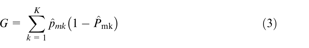
where ${\hat{P}}_{mk}$ represents the proportion of training observations in the $m^{th}$ region in the $k^{th}$ class.

The maximum depth of a tree is set to five to prevent overfitting where max depth gives the maximum depth up to which a tree can grow.³⁶ In order to achieve the best results in the test data set, we tried values from 2 to 10 for maximum depth parameter so as to cover a wide range of possibilities.

In the RF algorithm, a number of trees (number of iterations) are set to 100 which used the same parameters of splitting decision and the maximum depth of the DT. Using more than 100 models in RF algorithm did not improve the results.

The learning rate is taken as 0.12 and 100 models are built in a GB Algorithm. As the case of RF algorithm; 100 models did not improve the results of GB algorithm. Among the tested learning rates (0.01–0.5), a learning rate of 0.12 gave the best accuracy results for GB.

For the SVM algorithm, the radial basis kernel function outperforms the kernel functions of linear, polynomial of order two and three and sigmoid function. Another important support vector classifier (SVC) parameter is regularization parameter C changing the regularization parameter affects the shape of the function. While High values of C results in more smooth functions, low values result in more complex functions leading to overfitting problems. In our experiments, we found that the best C value is 1.0. Results of the algorithms are summarized in figures and tables below.

Next, we will fit a classification model in order to predict pump condition using delay (lag) functions need to be created from data sources including timestamps. Lag features are the classical way that time series forecasting problems are transformed into supervised learning problems. The simplest approach is to predict the value at the next time (t+1) given the value at the previous time (t).

The discussion begins with analyzing the numerical and graphical summaries that resulted from applying ML algorithms for the bearings data. For each recorded data, we have predicted the fault occurrence recognized by pump operating conditions for the nine previous hours, Lag 1 through Lag 9. Now we compare the algorithms’ performance across five random train-test splits of the data using classification accuracy. Figure 7 presents the output of accuracy for every nine lags expressed as the probability of correct classification. As the figure indicates, the GB and RF achieved slightly more than 88% mean accuracy in Lag 1, associated with the correct detection of critical bearing conditions before 1 h. On the other hand, SVM and DT respectively resulted in 82.2% and 81.9% mean accuracy giving an initial indication that DT gives the worse accuracy compared with the other three algorithms. A more extensive analysis of the algorithm’s performance is presented later in the Performance Measures section.

Figure 7.

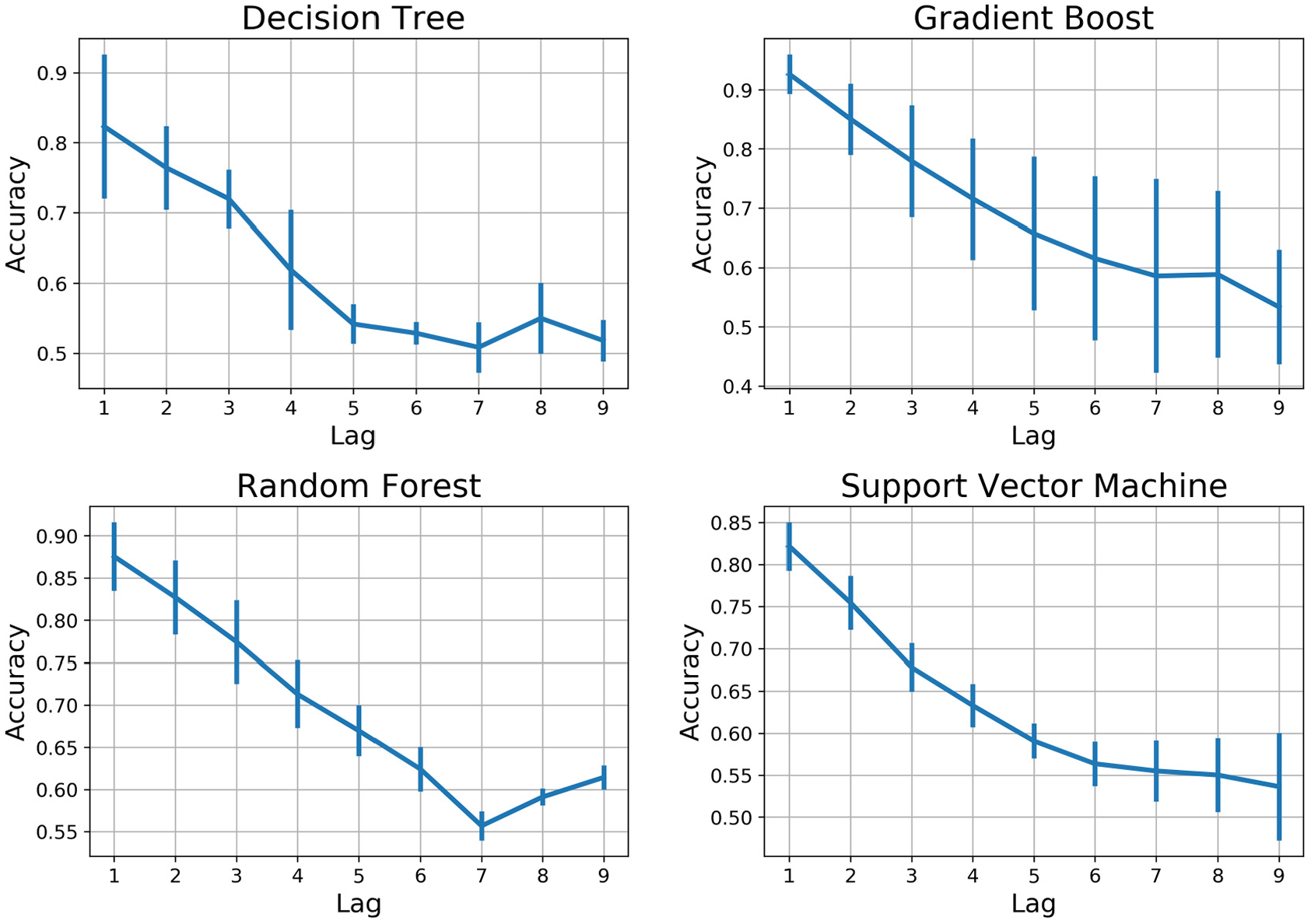
Comparison of ML algorithms performance with respect to their accuracy-lag.

In general, we can see that the prediction accuracy for all models is decreasing significantly with increasing the lag number from one to nine reaching minimum prediction accuracy less than 53% at lag 9. This is a logical consequence since many unexpected circumstances might appear when the prediction took place earlier. Table 3 summarizes the mean and standard deviation (SD) for all ML models for nine lags.

Table 3.

The mean and standard deviation for all ML models for nine lags.

DT algorithm	Mean	SD	GB algorithm	Mean	SD
Lag 1	0.819	0.102	Lag 1	0.926	0.034
Lag 2	0.759	0.058	Lag 2	0.85	0.06
Lag 3	0.707	0.031	Lag 3	0.779	0.095
Lag 4	0.616	0.075	Lag 4	0.716	0.102
Lag 5	0.543	0.032	Lag 5	0.658	0.129
Lag 6	0.518	0.022	Lag 6	0.616	0.139
Lag 7	0.511	0.043	Lag 7	0.586	0.163
Lag 8	0.544	0.051	Lag 8	0.589	0.141
Lag 9	0.524	0.017	Lag 9	0.534	0.097
RF algorithm	Mean	SD	SVM algorithm	Mean	SD
Lag 1	0.876	0.031	Lag 1	0.822	0.029
Lag 2	0.826	0.045	Lag 2	0.755	0.032
Lag 3	0.767	0.041	Lag 3	0.678	0.029
Lag 4	0.729	0.027	Lag 4	0.633	0.026
Lag 5	0.672	0.025	Lag 5	0.591	0.021
Lag 6	0.611	0.042	Lag 6	0.564	0.027
Lag 7	0.569	0.023	Lag 7	0.555	0.037
Lag 8	0.595	0.014	Lag 8	0.55	0.044
Lag 9	0.61	0.015	Lag 9	0.536	0.064

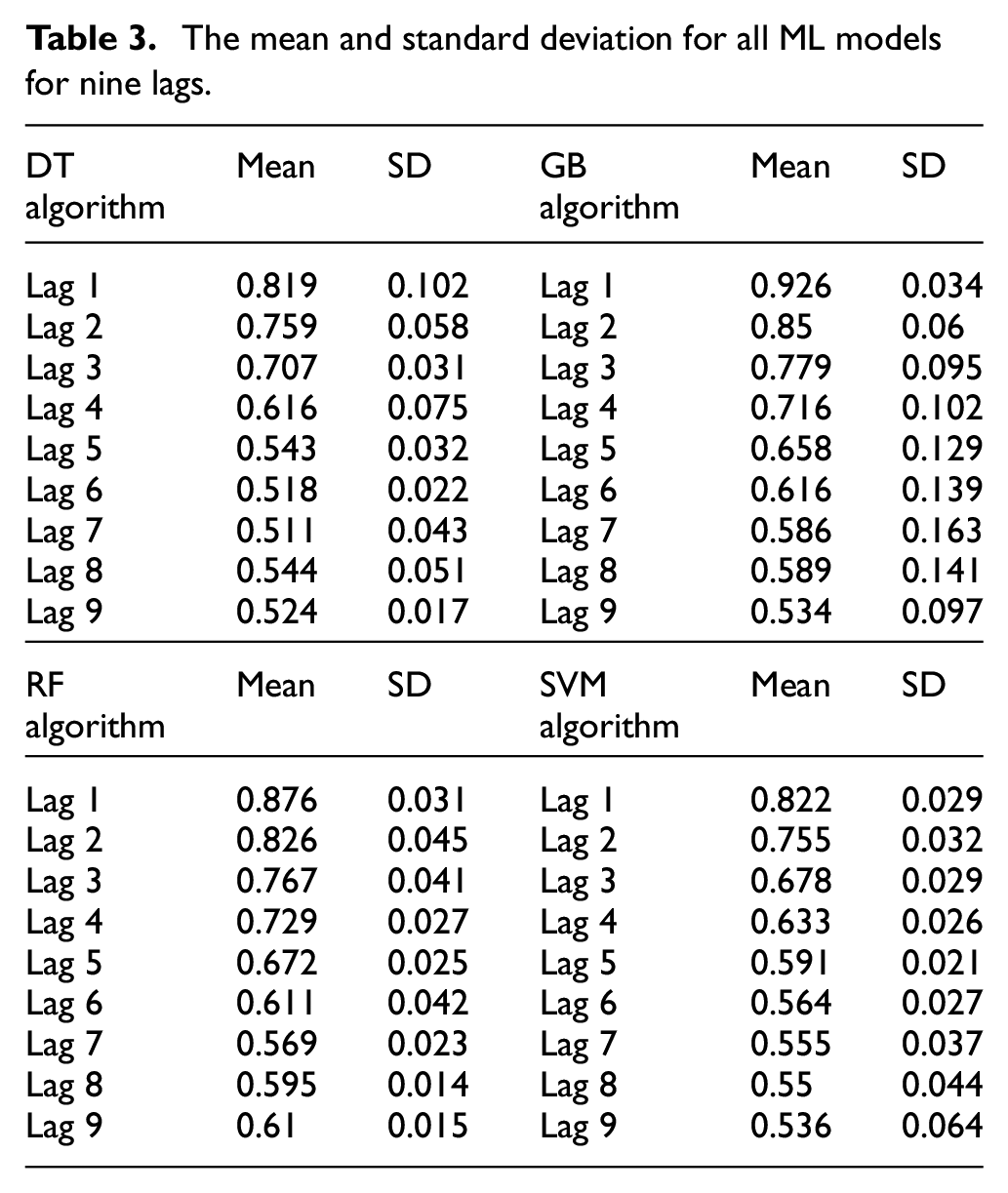
For the purpose of comparing algorithms performance, it is important to consider both mean and SD values. The higher the SD, the less precise is the prediction estimate. For example, although the mean value for GB is better than RF, the SD in RF is less indicating a more precise estimation. To compare the overall performance of both algorithms, a confidence interval may be useful to draw the conclusion.

Performance measures

Several performance measures are used to compare and evaluate the power of model prediction. As mentioned earlier, four distinct models are developed to predict if the operating condition is critical or normal where the maintenance is performed or delay accordingly. The training results of an application are compared in terms of the predictive performance for the testing accuracy of the classifiers algorithm. In the analysis accuracy (%) is considered as a performance index and is computed as:

Accuracy = (TP + TN) / (TP + FP + TN + FN)

(4)

where TP, TN, FP, and FN are true positive, true negative, false positive, and false negative rates, respectively. The accuracy is thus a combination of precision (or positive predictive value) and recall (sensitivity) measures.⁷¹ The precision determines the exactness of the model. It is a ratio of correctly predicted positive instances (TP) to the total positively predicted instances (TP + FP). Precision is represented as:

Precision = TP / (TP + FP)

(5)

In contrast, recall provides a measure of the model’s completeness. It is a ratio of a correctly predicted positive instance to the total instance of the positive class (TP + FN) in test data. A recall is calculated as:

Recall = TP / (TP + FN)

(6)

Precision represents the model’s performance with respect to false positives, whereas recall represents the performance with respect to false negatives. The F₁-score conveys the balance between precision and recall by taking their weighted sum. F₁-score is calculated as follows:

F_{1} = (2 * Precision * Recall) / (Precision + Recall)

(7)

Similar to the accuracy, F₁-score performs well with the fairly balanced dataset. Given the performance evaluation measures, the idea is to maximize the TP and TN and minimize the FN and FP. Generally, a reasonable tradeoff between the FP and TN risks is needed for better predictability. In the case of maintenance, however, the false negative (i.e. when the model predicts no need for maintenance, where it is needed) is more critical. Finally, in our experiments, we also compute the receiver operating characteristic curve ROC (a.k.a Area under the curve AUC), which is a measure of the model’s performance based on the tradeoffs between TP and TN rates over all possible risk thresholds between 0% and 100%. In the ML community, a ROC over 0.70 is considered good, and a ROC over 0.80 is very good.⁴⁴

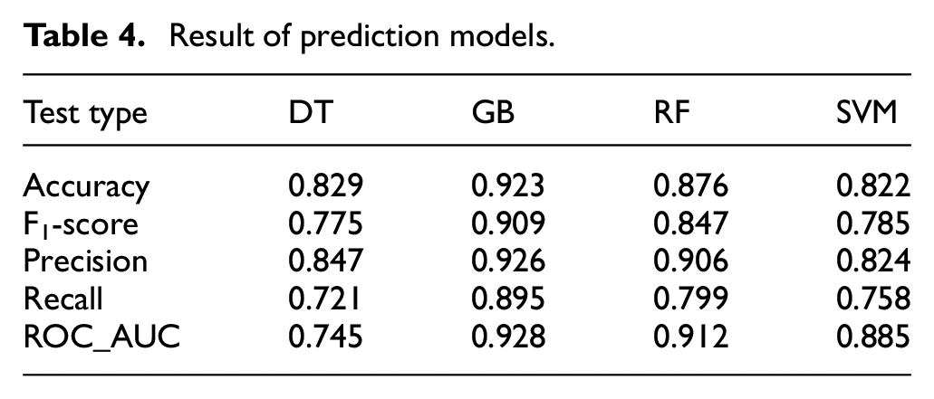
Table 4 shows the model evaluation results tested on a cross-validation dataset. All models show a negligible difference in performance. The GB model performs best in terms of all performance indicators where it reaches an accuracy of 92%; precision of 92.6% has an F-score and Recall of 91% and 89.5%, respectively. This supports our previous conclusion that the GB approach outperforms the other tested ML models. The SVM model, on the other hand, shows the lowest accuracy rate nearly to 82% as such as to the other evaluation criteria. Therefore, GB and RF showed the best performance indicators, with almost identical measures, and are found to outperform the other two models. It is also noteworthy that even with the worst ML model, DT, the AUC measure is considered acceptable (>0.7). ROC curves plots are used in order to evaluate the distinctive ability of the prediction, the GB model exhibits an even higher AUC (92.8%) while the DT model gives a lower AUC (74.5%) as shown in Figure 8 and Table 4.

Table 4.

Result of prediction models.

Test type	DT	GB	RF	SVM
Accuracy	0.829	0.923	0.876	0.822
F₁-score	0.775	0.909	0.847	0.785
Precision	0.847	0.926	0.906	0.824
Recall	0.721	0.895	0.799	0.758
ROC_AUC	0.745	0.928	0.912	0.885

Figure 8.

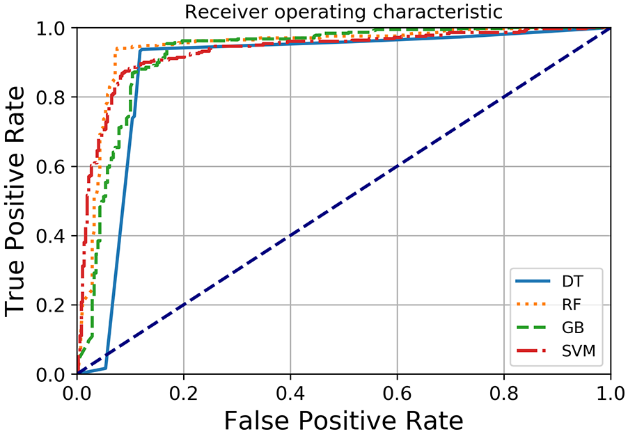
ROC curve of ML algorithms.

Decision making

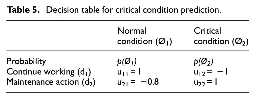
Once the ML algorithms are tested and the best approach is selected, the utility theory is integrated into our model to plan the maintenance action based on the probability of fault occurrence. Table 5 summarizes the utility matrix u_ij expressing the corresponding consequence for taking decision i given event j. Since it is less desirable to continue the machine work when the process is under a critical condition compared with taking a maintenance action when the process is normal, the utility (cost) for consequence u₁₂ is chosen to be less (higher) than that of u₂₁.

Table 5.

Decision table for critical condition prediction.

	Normalcondition (Ø₁)	Criticalcondition (Ø₂)
Probability	p(Ø₁)	p(Ø₂)
Continue working (d₁)	u₁₁ = 1	u₁₂ = −1
Maintenance action (d₂)	u₂₁ = −0.8	u₂₂ = 1

The probability p(Ø) represents how likely event i is to happen given the status of the active features extracted in the offline training phase. There are several approaches to detect these probabilities such as Bayesian networks and neural network algorithms. In this paper, however, we utilize the score resulted from the ML, which is a reflection of the status of all extracted features, and use it as input to the utility theory-based decision making. It is worth noting that the final output of ML is binary 0, 1 classification depending on whether the resulted decimal score is less or greater than 0.5, respectively. However, the decimal score (before binary classification) can be utilized in the application of utility theory as probability of normal and critical conditions.

The choice of the utility value u_ij is based on the decision maker’s knowledge of the system under investigation. Obviously, continue working under normal condition and take a maintenance action under critical condition will receive the maximum utility 1. The worst consequence, on the other hand, happens when work continues on a machine under a critical condition which not only produces nonconforming items but also may cause extra damage in the machinery and production system. Therefore, a utility of −1 is selected for such a consequence. The choice of utility value for taking a maintenance action under normal conditions depends on the cost of unnecessary maintenance and its impact on the production flow but in most cases, it is less serious than working under critical conditions. In this study, a value of −0.8 has been arbitrarily chosen for computational illustration.

It is also worthy to mention that the attitude of decision makers toward risk can significantly influence the way utility scores are defined. For example, in situations where the production management seeks to maximize profit through increasing the production volume within short period (risk-seeking approach), an unnecessary maintenance act will be avoided and critical condition signs with relatively small probabilities will be disregarded. On the other hand, risk-averse decision-makers who follow a more conservative approach will be more protective against any risk of machine failure even with low probability and thus will assign higher utility to unnecessary maintenance action.

The current paper provides a general framework for integrating the concept utility theory with ML to improve decision making regarding PdM. Considering maintenance costs including inspection, repair, failure, and replacement costs; as well as decision-makers’ attitude to risks will help to provide an accurate estimate of the expected utility for each decision alternative. We highlight this as a gap for further extension and investigation.

Figure 9 shows the two expected utility curves for d₁ and d₂. Based on utility maximization rule we should take maintenance action when the expected utility for d₂ (maintenance action) becomes larger than d₁ (continue working). Thus, the maintenance action time can be identified by the intersection of two expected utility functions.

Figure 9.

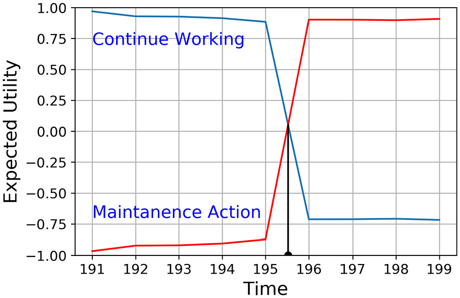
Expected utility for “continue working” and “maintenance action.”

Conclusions and future works

This paper utilizes ML techniques for the development of fault prediction models. Our models are based on estimations taken 1 to 9 h (Lag) in advance that give sufficient time for operators to prepare for inspections. This helps in taking the correct maintenance action on bearing components (e.g. checking the lubricant, cleaning the bearing housing, or preventing overheating) which will in turn increase bearings durability.

The prediction model has been implemented on a real industrial company which provided us with the necessary data collected using an online sensor measurement system. The proposed model has been achieved by training several ML algorithms on the python program. The computational analysis showed that the four ML approaches resulted in acceptable fault detection power. However, among the tested algorithms, GB and RF gave the best performance and accuracy: 92% and 87.6%, respectively. Using ML with the recorded maintenance data demonstrated that PdM could be done and provides good and reliable criteria for the maintenance planned interventions. The model aids operators to easily visualize and monitor the pumping system. Furthermore, while most of the related literature depends on their maintenance action only based on ML results (0, 1 binary classification), the current model is distinguished by its ability to show the probability of critical conditions through the use of utility theory. This helps to avoid false positive alarms and thus reduces the unnecessary maintenance costs. Therefore, this paper significantly contributes to achieving a more trustworthy maintenance management system for different Industrial applications. As a potential area for future research, the proposed fault detection methodology can be extended to include planning of maintenance schedules using a statistical cost minimization approach.

Footnotes

Acknowledgements

Authors of this study are extremely grateful to Sewerage Treatment Company/QATAR, for the provision of various data and information on the machines and equipment. Special thanks are due to Dr Mohanad Al-Ani for his assist. Ministry of Higher Education and Scientific Research of Iraq is gratefully acknowledged for the PhD study program of Raghad Mohammed Khorsheed.

Declaration of conflicting interests

The author(s) declared no potential conflicts of interest with respect to the research, authorship, and/or publication of this article.

Funding

The author(s) received no financial support for the research, authorship, and/or publication of this article.

ORCID iD

Omer Faruk Beyca

References

Rashid

Amar

Gondal

, et al. A data mining approach for machine fault diagnosis based on associated frequency patterns. Appl Intell 2016; 45(3): 638–651.

Hashemian

HM.

Wireless sensors for predictive maintenance of rotating equipment in research reactors. Ann Nucl Energy 2011; 38(2–3): 665–680.

Cong

Chen

Dong

, et al. Vibration model of rolling element bearings in a rotor-bearing system for fault diagnosis. J Sound Vib 2013; 332(8): 2081–2097.

Caesarendra

Kosasih

Tieu

, et al. Circular domain features based condition monitoring for low speed slewing bearing. Mech Syst Signal Process 2014; 45(1): 114–138.

Saruhan

Sandemir

Çiçek

, et al. Vibration analysis of rolling element bearings defects. J Appl Res Technol 2014; 12(3): 384–395.

Tran

Yang

B-S.

An intelligent condition-based maintenance platform for rotating machinery. Expert Syst Appl 2012; 39(3): 2977–2988.

Raposo

Farinha

Ferreira

, et al. Dimensioning reserve bus fleet using life cycle cost models and condition based/predictive maintenance: a case study. Public Transp 2018; 10(1): 169–190.

Sakib

Wuest

Challenges and opportunities of condition-based predictive maintenance: a review. Procedia CIRP 2018; 78: 267–272.

Wang

. A predictive production planning with condition-based maintenance in a deteriorating production system. In: 2016 international conference on robotics and automation engineering (ICRAE), 2016, pp.35–38. IEEE. DOI: 10.1109/ICRAE.2016.7738784.

10.

Qian

Tian

Kanfoud

, et al. A novel condition monitoring method of wind turbines based on long short-term memory neural network. Energies 2019; 12(18): 3411.

11.

Carnero

MC.

Selection of diagnostic techniques and instrumentation in a predictive maintenance program. A case study. Decis Support Syst 2005; 38(4): 539–555.

12.

Yiakopoulos

Gryllias

Antoniadis

IA.

Rolling element bearing fault detection in industrial environments based on a K-means clustering approach. Expert Syst Appl 2011; 38(3): 2888–2911.

13.

Carnero Moya

. The control of the setting up of a predictive maintenance programme using a system of indicators. Omega 2004; 32(1): 57–75.

14.

Zhao

Wang

Jia

, et al. Predictive maintenance policy based on process data. Chemom Intell Lab Syst 2010; 103(2): 137–143.

15.

Selcuk

Predictive maintenance, its implementation and latest trends. Proc IMechE, Part B: J Engineering Manufacture 2017; 231(9): 1670–1679.

16.

Voronov

Machine learning models for predictive maintenance. Sweden, 2020. http://urn.kb.se/resolve?urn=urn:nbn:se:liu:diva-162649.

17.

Orhan

Aktürk

Çelik

Vibration monitoring for defect diagnosis of rolling element bearings as a predictive maintenance tool: comprehensive case studies. NDT E Int 2006; 39(4): 293–298.

18.

Hassin

OAA

. Condition monitoring of journal bearings for predictive maintenance management based on high frequency vibration analysis, 2017, http://eprints.hud.ac.uk/id/eprint/34161/.

19.

NASA. Reliability centered maintenance. In: Engineering maintenance. CRC Press, 2008, P.472. DOI: 10.1201/9781420031843.

20.

Caesarendra

Kosasih

Tieu

, et al. Acoustic emission-based condition monitoring methods: review and application for low speed slew bearing. Mech Syst Signal Process 2016; 72–73: 134–159.

21.

Ferrando Chacon

Kappatos

Balachandran

, et al. A novel approach for incipient defect detection in rolling bearings using acoustic emission technique. Appl Acoust 2015; 89: 88–100.

22.

Giannenas

Triantafillou

Stavrakakis

, et al. Assessment of dietary supplementation with carvacrol or thymol containing feed additives on performance, intestinal microbiota and antioxidant status of rainbow trout (oncorhynchus mykiss). Aquaculture 2012; 350–353(215): 26–32.

23.

Kalligeros

Predictive maintenance of hydraulic lifts through lubricating oil analysis. Machines 2013; 2(1): 1–12.

24.

Raposo

Farinha

Fonseca

, et al. Predicting condition based on oil analysis – a case study. Tribol Int 2019; 135: 65–74.

25.

Fantidis

Potolias

Bandekas

DV.

Wind turbine blade nondestructive testing with a transportable radiography system. Sci Technol Nucl Install 2011; 2011: 347320.

26.

Zhen

Zhengjia

Yanyang

, et al. Bearing condition monitoring based on shock pulse method and improved redundant lifting scheme. Math Comput Simul 2008; 79(3): 318–338.

27.

García Márquez

Tobias

Pinar Pérez

, et al. Condition monitoring of wind turbines: techniques and methods. Renew Energy 2012; 46: 169–178.

28.

Vianna

WOL

Yoneyama

. Predictive maintenance optimization for aircraft redundant systems subjected to multiple wear profiles. IEEE Syst J 2018; 12(2): 1170–1181.

29.

Salomon

Ferreira

Sant’Ana

, et al. A study of fault diagnosis based on electrical signature analysis for synchronous generators predictive maintenance in bulk electric systems. Energies 2019; 12(8): 1506.

30.

Tse

Peng

Yam

Wavelet analysis and envelope detection for rolling element bearing fault diagnosis—their effectiveness and flexibilities. J Vib Acoust 2001; 123(3): 303–310.

31.

Pappachan

Caesarendra

Tjahjowidodo

, et al. Frequency domain analysis of sensor data for event classification in real-time robot assisted deburring. Sensors 2017; 17(6): 1247.

32.

Patidar

Soni

An overview on vibration analysis techniques for the diagnosis of rolling element bearing faults. Int J Eng Trends Technol 2013; 4(5): 1804–1809.

33.

Dong

Mingyue

Guoying

Application of internet of things technology on predictive maintenance system of coal equipment. Procedia Eng 2017; 174: 885–889.

34.

Amruthnath

Gupta

. A research study on unsupervised machine learning algorithms for early fault detection in predictive maintenance. In: 2018 5th international conference on industrial engineering and applications (ICIEA). IEEE, 2018, pp.355–361. DOI: 10.1109/IEA.2018.8387124.

35.

Chen

An internet of things based framework to enhance just-in-time manufacturing. Proc IMechE, Part B: J Engineering Manufacture 2018; 232(13): 2353–2363.

36.

Murty

Devi

VS.

Introduction to pattern recognition and machine learning. Vol 5. Co-published with Indian Institute of Science (IISc), Bangalore, India, 2015. DOI: 10.1142/8037.

37.

Baptista

Sankararaman

de Medeiros

, et al. Forecasting fault events for predictive maintenance using data-driven techniques and ARMA modeling. Comput Ind Eng 2018; 115: 41–53.

38.

Van Every

Rodriguez

Jones

, et al. Advanced detection of HVAC faults using unsupervised SVM novelty detection and Gaussian process models. Energy Build 2017; 149: 216–224.

39.

Susto

Schirru

Pampuri

, et al. Machine learning for predictive maintenance: a multiple classifier approach. IEEE Trans Ind Informatics 2015; 11(3): 812–820.

40.

Tian

Gao

, et al. Fault detection of oil pump based on classify support vector machine. In: 2007 IEEE international conference on control and automation, 2007, pp.549–553. IEEE. DOI: 10.1109/ICCA.2007.4376416.

41.

Samantaray

SR.

Ensemble decision trees for high impedance fault detection in power distribution network. Int J Electr Power Energy Syst 2012; 43(1): 1048–1055.

42.

Parikh

, et al. Improving rail network velocity: a machine learning approach to predictive maintenance. Transp Res Part C Emerg Technol 2014; 45: 17–26.

43.

Kroll

Schaffranek

Schriegel

, et al. System modeling based on machine learning for anomaly detection and predictive maintenance in industrial plants. In: Proceedings of the 2014 IEEE emerging technology and factory automation (ETFA), 2014, pp.1–7, IEEE. DOI: 10.1109/ETFA.2014.7005202.

44.

Cline

Niculescu

Huffman

, et al. Predictive maintenance applications for machine learning. In: 2017 annual reliability and maintainability symposium (RAMS), 2017. IEEE. DOI: 10.1109/RAM.2017.7889679.

45.

Paolanti

Romeo

Felicetti

, et al. Machine learning approach for predictive maintenance in industry 4.0. In: 2018 14th IEEE/ASME international conference on mechatronic and embedded systems and applications (MESA), 2018. IEEE. DOI: 10.1109/MESA.2018.8449150.

46.

Allah Bukhsh

Saeed

Stipanovic

, et al. Predictive maintenance using tree-based classification techniques: a case of railway switches. Transp Res Part C Emerg Technol 2019; 101: 35–54.

47.

Gutschi

Furian

Suschnigg

, et al. Log-based predictive maintenance in discrete parts manufacturing. Procedia CIRP 2019; 79: 528–533.

48.

Xayyasith

Promwungkwa

Ngamsanroaj

. Application of machine learning for predictive maintenance cooling system in Nam Ngum-1 hydropower plant. In: 2018 16th international conference on ICT and knowledge engineering (ICT&KE), 2018. IEEE. DOI: 10.1109/ICTKE.2018.8612435.

49.

Nam

Kim

, et al. Development of a health monitoring and diagnosis framework for fused deposition modeling process based on a machine learning algorithm. Proc IMechE, Part B: J Engineering Manufacture 2020; 234(1–2): 324–332.

50.

Caesarendra

Tjahjowidodo

A review of feature extraction methods in vibration-based condition monitoring and its application for degradation trend estimation of low-speed slew bearing. Machines 2017; 5(4): 21.

51.

Finley

Hodowanec

Holter

WG.

An analytical approach to solving motor vibration problems. IEEE Trans Ind Appl 2000; 36(5): 1467–1480.

52.

Sheng

Rovnyak

SM.

Decision tree-based methodology for high impedance fault detection. IEEE Trans Power Deliv 2004; 19(2): 533–536.

53.

Kotsiantis

Zaharakis

Pintelas

PE.

Supervised machine learning: a review of classification techniques general issues of supervised learning algorithms. Inform 2007; 31: 249–268.

54.

Gerdes

Decision trees and genetic algorithms for condition monitoring forecasting of aircraft air conditioning. Expert System Appl 2013; 40(12): 5021–5026.

55.

Prytz

Nowaczyk

Rögnvaldsson

, et al. Predicting the need for vehicle compressor repairs using maintenance records and logged vehicle data. Eng Appl Artif Intell 2015; 41: 139–150.

56.

Patel

Jokhakar

. A random forest based machine learning approach for mild steel defect diagnosis. In: 2016 IEEE international conference on computational intelligence and computing research (ICCIC), 2016. IEEE. DOI: 10.1109/ICCIC.2016.7919549.

57.

Kejela

Esteves

Rong

. Predictive analytics of sensor data using distributed machine learning techniques. In: 2014 IEEE 6th international conference on cloud computing technology and science, vol. 2015, 2014, pp.626–631. IEEE. DOI: 10.1109/CloudCom.2014.44.

58.

Natekin

Knoll

Gradient boosting machines, a tutorial. Front Neurorobot 2013; 7. DOI: 10.3389/fnbot.2013.00021.

59.

Susto

Schirru

Pampuri

, et al. A predictive maintenance system for integral type faults based on support vector machines: an application to ion implantation. In: 2013 IEEE international conference on automation science and engineering (CASE), 2013, pp.195–200. IEEE. DOI: 10.1109/CoASE.2013.6653952.

60.

Kotsiantis

Zaharakis

Pintelas

PE.

Machine learning: a review of classification and combining techniques. Artif Intell Rev 2006; 26(3): 159–190.

61.

Granderson

Auslander

, et al. Design of machine learning models with domain experts for automated sensor selection for energy fault detection. Appl Energy 2019; 235: 117–128.

62.

Baccarini

LMR

Avelar

Silva

VVRE

, et al. Intelligent system design for stator windings faults diagnosis: suitable for maintenance work. J Softw Eng Appl 2013; 6(10): 526–532.

63.

Hatamura

Decision-making in engineering design: theory and practice. London: Springer, 2006.

64.

Kong

Beyca

Bukkapatnam

, et al. Nonlinear sequential Bayesian analysis-based decision making for end-point detection of chemical mechanical planarization (CMP) processes. IEEE Trans Semicond Manuf 2011; 24(4): 523–532.

65.

Lindley

DV.

Making decisions. 2nd ed. London: Wiley, 1985.

66.

de Almeida

Bohoris

. Decision theory in maintenance decision making. J Qual Maint Eng 1995; 1(1): 39–45.

67.

Kuhn

Johnson

Applied predictive modeling. New York, NY: Springer, 2013.

68.

Ahmed

Baqqar

, et al. Fault detection and diagnosis using principal component analysis of vibration data from a reciprocating compressor. In: Proceedings of 2012 UKACC international conference on control, 2012, pp.461–466. IEEE. DOI: 10.1109/CONTROL.2012.6334674.

69.

Manco

Ritacco

Rullo

, et al. Fault detection and explanation through big data analysis on sensor streams. Expert System Appl 2017; 87: 141–156.

70.

James

Witten

Hastie

, et al. An introduction to statistical learning, vol. 103, 2013. DOI: 10.1007/978-1-4614-7138-7.

71.

Sokolova

Lapalme

A systematic analysis of performance measures for classification tasks. Inf Process Manag 2009; 45(4): 427–437.

An integrated machine learning: Utility theory framework for real-time predictive maintenance in pumping systems

Abstract

Keywords

Introduction

Related work

Research methodology

Offline model training

ML algorithms

Decision Trees (DT)

Random Forest (RF)

Gradient Boosted (GB)

Support Vector Machines (SVM)

Decision-making theory

Case study

Data collection and preprocess

Dimension reduction

Building classification algorithm

Performance measures

Decision making

Conclusions and future works

Footnotes

Acknowledgements

Declaration of conflicting interests

Funding

ORCID iD

References