Sage Journals: Discover world-class research

Abstract

Ball screws play a critical role in high-quality precision manufacturing. The use of machine learning and artificial intelligence for the diagnosis of machines’ health status is increasingly pertinent. The processing of big data originating from machine sensors is crucial. However, installing multiple sensors on the object requiring diagnosis may be costly. A sensorless strategy using built-in signals to determine the conditions of a hollow ball screw was deployed. Moreover, we evaluated the most discriminative parameters among fusion sensor signals by using Fisher’ criteria. A support vector machine (SVM) as diagnostic tool was used. In the absence of prominent characteristic features in data, the conventional SVM cannot classify the data well. To address this concern, we constructed a feature engineering for distinguishing features from the raw data to facilitate the SVM classification process well. In addition, we validated the physical phenomenon in realistic ball screw conditions through feature extraction. Experimental results demonstrated the average diagnostic accuracy levels for the ball screw preload, pretension, cooling system, and table payload were 98.91%, 94.08%, 91.69%, and 93.5%, respectively, after feature engineering was applied successfully.

Keywords

Hollow ball screw support vector machine Fisher criterion feature extraction

Introduction

Hollow ball screws, critical mechanical components deployed to convert rotary movement into linear movement, are crucial in the manufacturing industry. Under continuous operation, the preload stress of a ball screw causes thermal deformation and the phenomenon can subsequently affect position accuracy when ball screw pretension was lost. Wei et al.¹ analyzed the mechanical performance of ball screw elements, such as contact angles and the friction coefficients of ball-screw and ball-nut contact areas. Hilbert–Huang Transform (HHT) was employed in processing signals to investigate the faults and mechanisms of a ball screw.^2,3 Use of ball screw preload for the increase of mechanical stiffness of is usually deployed for a feed drive system. Since the ball screw preserves the lowest stiffness of the feed drive system. The positioning error of a ball screw caused by thermal expansion can deteriorate the positioning accuracy of a feed drive system. Use of ball screw pretension for thermal elongation was usually deployed for ball screw compensation. Since loss of ball screw pretension reveals positioning error before any controller effort. Though prediction models for positioning error or on-line compensation method were studied for positioning compensation.^4,5 However, the health assessment such as preload loss, thermal expansion, cooling system malfunction or fast removing cutting material of the ball screw is pretty crucial and is a must before the control compensation. Since these may cause position error, lower axial mechanical stiffness, lower frequency bandwidth, unbalanced thermal stress and strain and changed natural frequency. All of such render the bad operation status of the CNC machine tool in practice. Especially, with the trend of industrial 4.0 prognostic diagnosis demand accelerates the big data collection for knowing the machine health status.

With the rise of artificial intelligence, productive maintenance strategies have emerged, and the diagnosis of machines’ health status has become a pertinent topic. Wang and Vachtsevanos⁶ performed prognostic diagnosis on a rolling element fault using a recurrent wavelet neural network. Tsai et al.⁷ proposed angular-velocity Vold–Kalman filtering order tracking to monitor changes in ball pass frequency to detect any preload loss in the ball screw. Compared with other algorithms for fault diagnosis, the support vector machine (SVM) has gained popularity owing to its effective classification performance and the little training and testing time required.⁸ The best property of SVM is that it is particularly effective in classifying different classes despite the limited training and small amount of testing data. The small amount of data also reduced the computational load.⁹

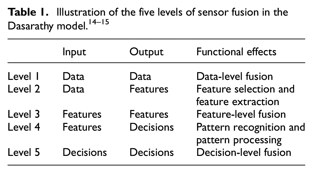
Wang et al.¹⁰ presented an ensemble SVM to classify four image blur types and demonstrated its superior performance by comparing it with a standard SVM and other state-of-the-art blur classification methods. Patel and Upadhyay¹¹ compared an artificial neural network (ANN) and SVM for fault diagnosis in rolling element bearings. Experimental results revealed that the SVM method had a more favorable classification capability than the backpropagation ANN despite the limited training sample size. However, the SVM algorithm is not always advantageous. Selection of the parameter values for different kernel functions and penalty issues in cost parameters are essential for the performance of the SVM. No standard operation process or methodology to set up these values exists.¹² Each classification problem of the SVM corresponds to an optimal parameter set. Moreover, the diagnostic accuracy of the SVM will not be ideal if the training data of different classes are ambiguous or not distinguished. To address these concerns, this paper describes the construction of feature engineering, which is based on the concept of data mining for extending dimensions of raw data. This is followed by choosing the optimal combination characteristic features among the extended data set. Therefore, the inputs of SVM was based on the concept of data mining for extending dimensions of raw data and abstracted features will be a bettering data cleaning solution for the SVM accuracy. Knowledge discovery databases (KDDs),^13–15 as shown in Figure 1, refers to a model for data fusion involving feature extraction and feature selection. Table 1 presents the five levels of sensor fusion. First, in level one to level three, input and output data go to the data driven to features, and feature selection is followed by feature extraction; a decision must be made in the level four and five. Recently, many researchers have diagnosed mechanical faults based on KDDs or data fusion.^16–18 Data preprocessing is a more robust and intelligent means for diagnosis, particularly with the rise of artificial intelligence.

Figure 1.

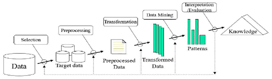
Overview of steps for compose the KDD process.¹³

Table 1.

Illustration of the five levels of sensor fusion in the Dasarathy model.^14–15

	Input	Output	Functional effects
Level 1	Data	Data	Data-level fusion
Level 2	Data	Features	Feature selection andfeature extraction
Level 3	Features	Features	Feature-level fusion
Level 4	Features	Decisions	Pattern recognition andpattern processing
Level 5	Decisions	Decisions	Decision-level fusion

In this research, a three-phase method for prognostic diagnosis is proposed. In the first phase, a single-axis ball screw was deployed to run in a repetitive motion by reciprocating the table’s travel distance for 5, 30, and up to 60 min. Three build-in-signal acquisitioned data by the linear scale position signal, motor current, and motor speed were obtained. Then, Fisher’s criteria were employed to investigate the most discriminating data among the three build-in-signal data sets. The most featured signal will be used for diagnosis. The second phase is to reduce the warm-up time for the startup feed drive efficiently, a repetitive, realistic short traveling distance for mimicking the shop floor machining path was proposed. This design experimental work will benefit industrial application and academic research when they conduct the health status of machine tools in a short time. In phase three, a systematic feature engineering extraction was implemented to expand the sensor dimensions of only the motor current data with a repetitive, realistic short traveling distance was deployed thereof. Finally, the process of feature engineering can promote the discrimination between the different classes we intended to classify and consequently lead to the SVM having an improved classification performance.

SVM method

Vapnik^19,20 first introduced a linear classifier based on statistical learning, the SVM, that can be used to differentiate between various classes. The original SVM was developed to solve binary classification problems by seeking the optimal separating hyperplane that divides different data classes. In a straightforward binary classification problem, such as in Figure 2, the hyperplane can separate the set of vectors without introducing any errors, if the margin is maximal. The brief mathematical model of the SVM is presented as follows.²¹

Figure 2.

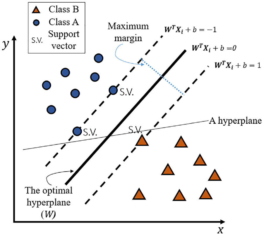
Illustration of a linearly separable SVM.

Given a binary classification problem with a data set $X_{i}$ (i =1, 2,……,n) belong to class A or class B, and their data point label is y_i = ±1. Equation (1) can satisfy the data point of this binary classification problem, where $W^{T}$ stands for the vector set of the optimal hyperplane; b is the bias.

y_{i} (W^{T} X_{i} + b) \geq 0 \forall_{i}

(1)

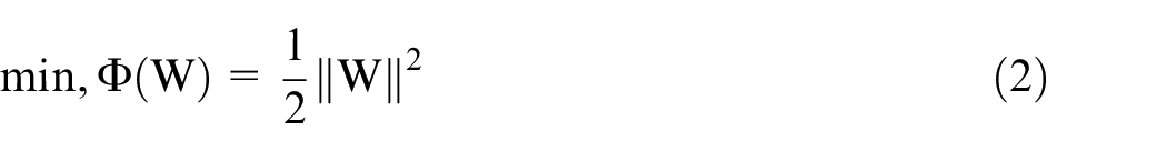
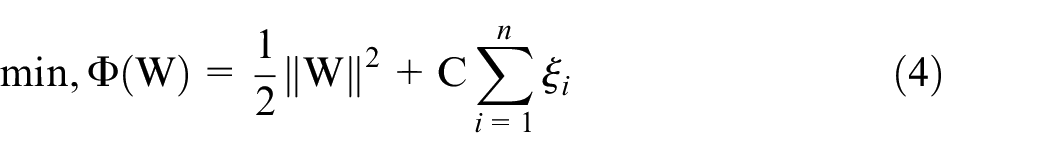
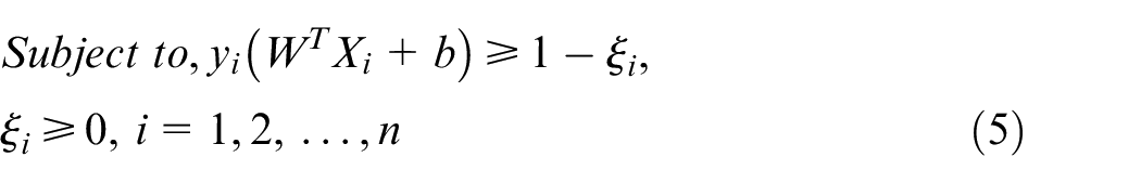
The goal of an SVM is to generate an optimal hyperplane with the maximal margin. This is represented by equations (2) and (3). Also, equations (2) and (3) are the models for the definition of the hard-margin SVM.

\min, Φ (W) = \frac{1}{2} ‖ W ‖^{2}

(2)

Subject to, y_{i} (W^{T} X_{i} + b) \geq 1, i = 1, 2, \dots, n

(3)

However, most real-world classification problems are nonlinear, not easily separable, and contain unexpected data that lead to misclassification. As a result, parameters C and $ξ_{i}$ were introduced to address the aforementioned issue. Equations (4) and (5) are the models for the soft-margin SVM, where $ξ_{i}$ is the slack variable that is introduced to allow misclassification for the whole data set. Every diagnosis point corresponds to the value of its slack variable. A user-defined cost parameter C can affect the extent of the maximal margin and decide the influence of the slack variables.

\min, Φ (W) = \frac{1}{2} ‖ W ‖^{2} + C \sum_{i = 1}^{n} ξ_{i}

(4)

\begin{matrix} Subject to, y_{i} (W^{T} X_{i} + b) \geq 1 - ξ_{i}, \\ ξ_{i} \geq 0, i = 1, 2, \dots, n \end{matrix}

(5)

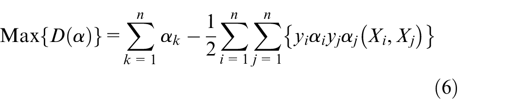
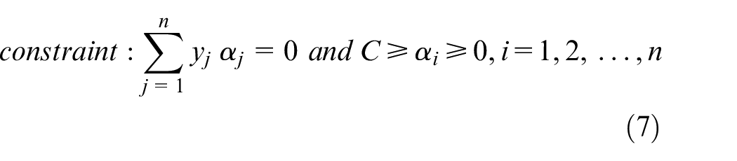
To reduce the complexity in equations (4) and (5), they can be converted into the equivalent Lagrange dual problem in equations (6) and (7), where $(X_{i}, X_{j})$ means the inner product of $X_{i}$ and $X_{j}$ , where the Lagrange multiplier, $α$ , must be found to maximize the ${D (α)}$ ²² subject to the constraints in equation (7).

Max {D (α)} = \sum_{k = 1}^{n} α_{k} - \frac{1}{2} \sum_{i = 1}^{n} \sum_{j = 1}^{n} {y_{i} α_{i} y_{j} α_{j} (X_{i}, X_{j})}

(6)

constraint : \sum_{j = 1}^{n} y_{j} α_{j} = 0 and C \geq α_{i} \geq 0, i = 1, 2, \dots, n

(7)

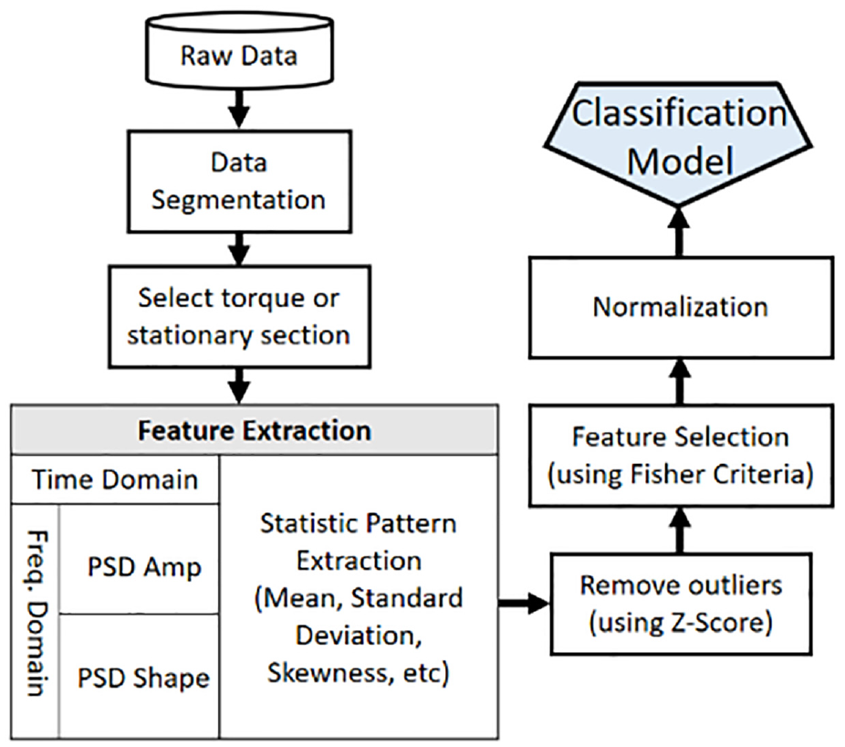
On the basis of the training set of $X_{i or j}$ and y_{i or j}, the optimal hyperplane of the SVM associated with $α$ was developed.

Feature engineering method

The core concept of feature engineering is to identify the most discriminative features from raw data by using a systematic operation. The fusing of different sensor signals features is discussed prominently in recent research. Those signals are obtained from different sensors when it is unclear which one is the key sensing signal for the characteristics of the object requiring diagnosis. Researchers^16–18 have constructed a flow chart for the feature engineering procedure presented in Figure 3.

Figure 3.

Flow chart of feature engineering.^16–18

Data segmentation

A realistic experimental figure is shown in Figure 4. The ball screw moves in a reciprocating motion within a fixed distance. Therefore, the acceleration, constant velocity and deceleration occurs during the duration of linear ball screw motion. Denoting torque part indicates the acceleration and deceleration duration while the stationary part is the time in constant velocity motion of the ball screw. Filtered raw data by stationary part of different ball screw were analyzed as follows.

Figure 4.

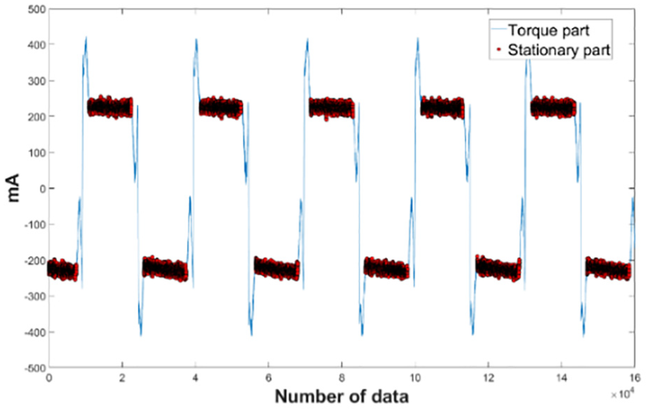
Torque and stationary parts.

In this step, raw data are divided into several segments with a constant number to acquire the signals of the torque or stationary part for future analysis. This was done by filtering the data-to-be-analyzed with six times of the averaged standard deviation window. To put it more specifically, first, we evenly divided the 160,000 raw data into 32 segments and calculated the average standard deviation for all segments. Then, remove the most likely signal outliners for every segment. They were filtered out by moving the threshold window of six standard deviations. Then the original data are initially cleaning and then go to the next feature expansion and extraction.

Feature extraction

First, all the statistical features are extracted from time domain, frequency domains, PSD-Amp and PSD-Shape. The flowchart for these steps is illustrated in Figure 5.

Figure 5.

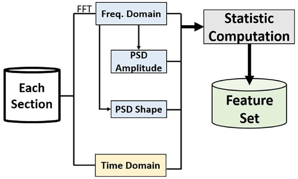
Flowchart of feature extraction.

Six statistical features, namely root mean square (RMS), kurtosis, variance, crest factor, standard deviation and skewness, are calculated and extracted in each section of time domain. These six features are denoted on the number 1 to number 6 of the Table 2. Another eight statistical features by mean, standard deviation, skewness, and kurtosis for the power spectrum density as PSD-Amp and PSD-Shape are denoted by the number 87 to 94 of the Table 2. Since some features calculated by the statistical points of view may arise from the change of mechanical properties of the ball screw feed drive system.

Table 2.

All 94 features for each data segment.

Number	Feature
1	RMS
2	Kurtosis
3	Variance
4	Crest factor
5	Standard deviation
6	Skewness
7~86	The average amplitude of frequency sectors $[1 + 50 * (i - 1)] Hz ~ (50 * i) Hz$ , $i = 1, 2, 3, \dots \dots, 80$
87	PSD – Amplitude mean
88	PSD – Amplitude standard deviation
89	PSD – Amplitude skewness
90	PSD – Amplitude Kurtosis
91	PSD – Shape mean
92	PSD – Shape standard deviation
93	PSD – Shape skewness
94	PSD – Shape Kurtosis

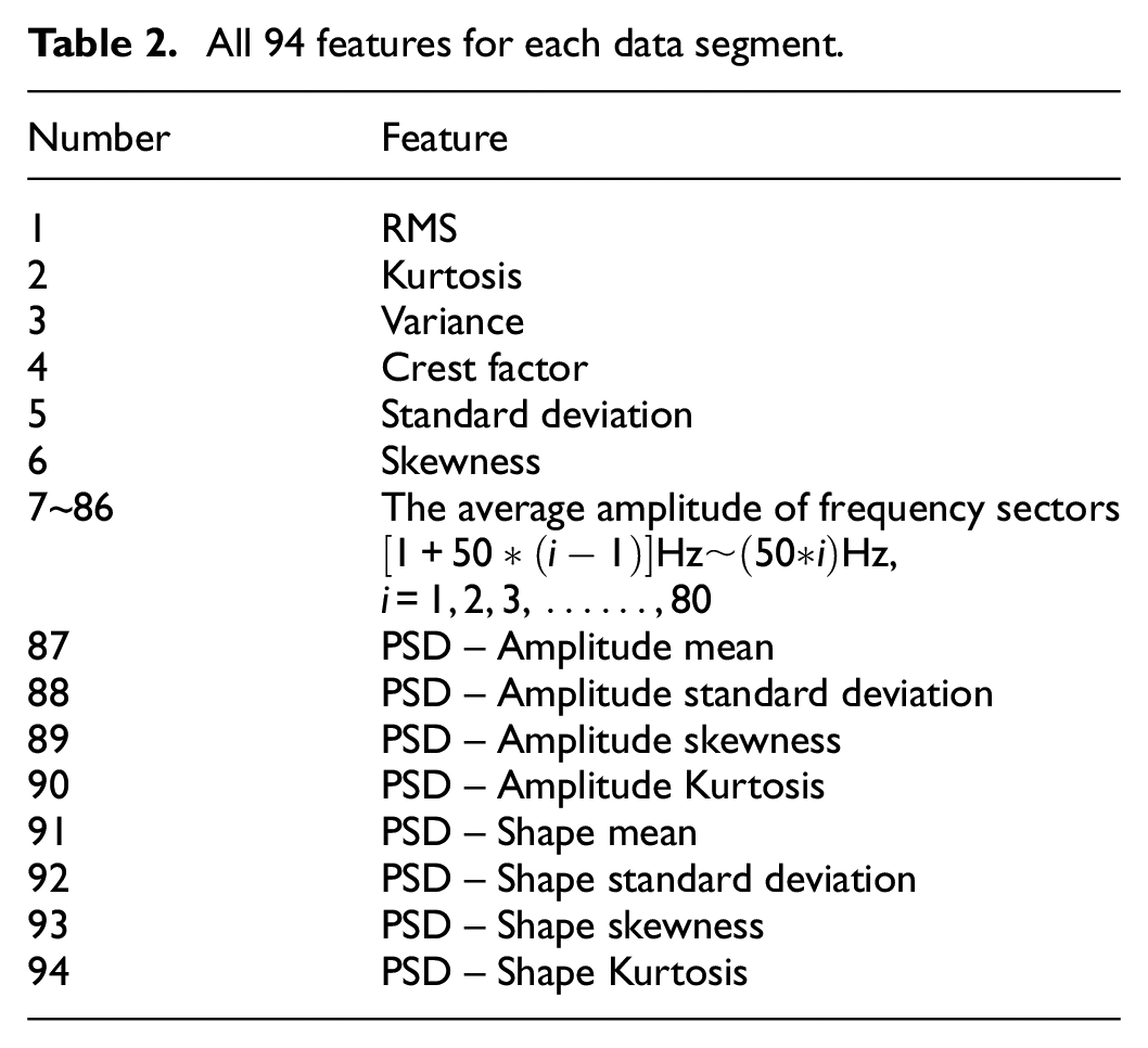
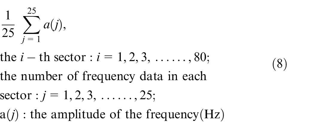
As mentioned, loss of preload, namely lower mechanical stiffness, will degrade the natural frequency of the whole feed drive system. Thus, data calculated for the frequency domain are averagely divided into 80 parts. These 80 features are denoted as the number 7 to number 86 of the Table 2. In each section, the mean of the value of the sum amplitude is a feature. The computational process is shown in equation (8).

\begin{matrix} \frac{1}{25} \sum_{j = 1}^{25} a (j), \\ the i - th sector : i = 1, 2, 3, \dots \dots, 80; \\ the number of frequency data in each \\ sector : j = 1, 2, 3, \dots \dots, 25; \\ a (j) : the amplitude of the frequency (Hz) \end{matrix}

(8)

Finally, 94 features are extracted for each data segment. All the features are listed in Table 2.

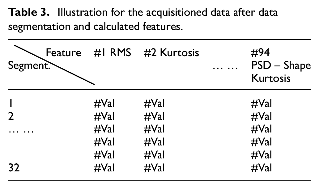
When we operate the data segmentation and feature extraction, we can construct a data table shown in Table 3.

Table 3.

Illustration for the acquisitioned data after data segmentation and calculated features.

FeatureSegment.	#1 RMS	#2 Kurtosis	#94PSD – ShapeKurtosis
1	#Val	#Val	#Val
2	#Val	#Val	#Val
……	#Val	#Val	#Val
	#Val	#Val	#Val
	#Val	#Val	#Val
32	#Val	#Val	#Val

Outlier reduction

In this step, outliers of each feature type are removed using Z-score to avoid their interference in the training of the algorithm. The Z-score formula is shown in function (9).

Z - Score = \frac{x_{i} - μ}{σ_{s}}

(9)

$x_{i}$ represents the i-th section in the feature, $μ$ denotes the mean of the feature, and $σ_{s}$ is the standard deviation of the feature. In each section of the feature, if the Z-score value exceeds the interval set by the operator, the section is removed.

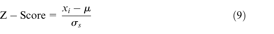
To explain this process specifically, the Z-score interval is set between +3 and −3 in this paper. For an example, we calculated the Z-Score of each segment for the column of # 1 RMS first. Since each segment stands for 160,000 divided by 32 data set. Secondly, we remove the whole segment (the row of Table 3 in #1 RMS) if there are one value bigger than +3 or less than −3. Then we repeat the steps until all features (from #1 to # 94) are processed.

Feature selection

In this step, the most discriminative feature among all features is selected by using Fisher’s criteria.²³ The formula is shown in equation (9).

FS = \frac{{(m_{2 -} m_{1})}^{2}}{s_{1}^{2} + s_{2}^{2}}

(10)

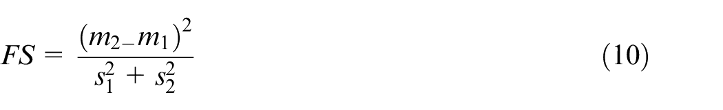
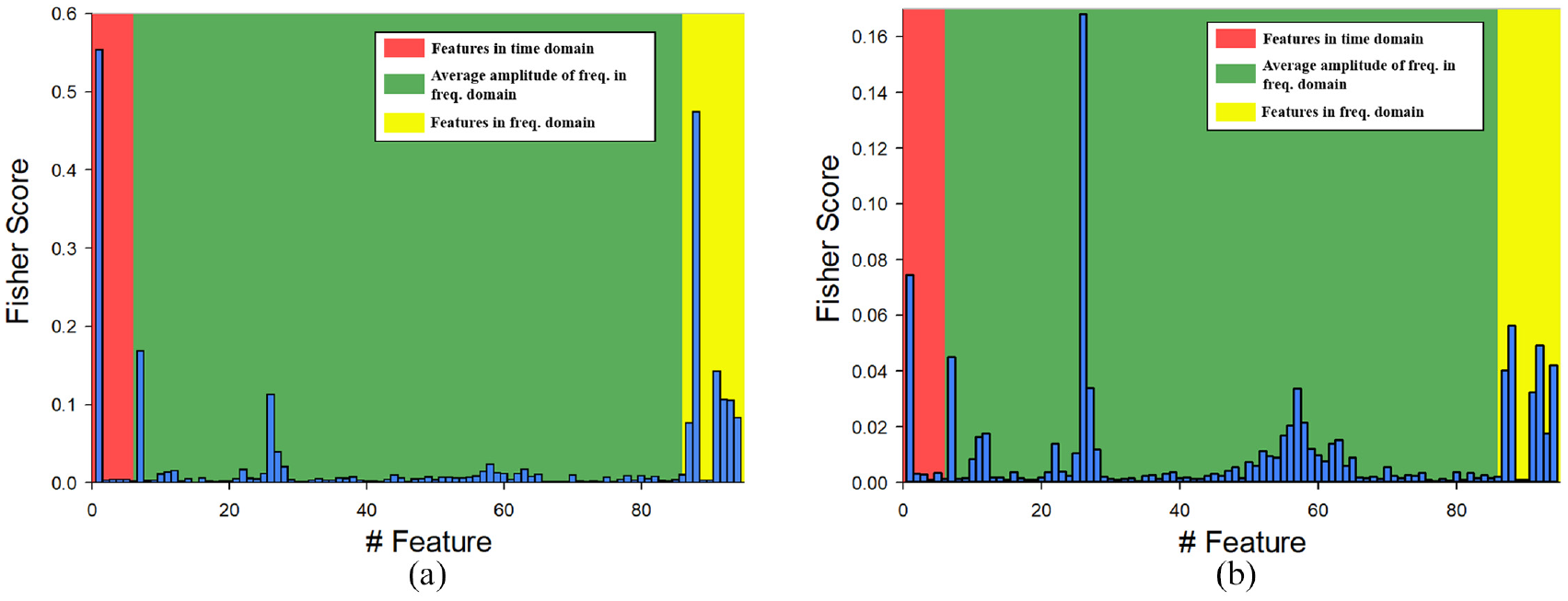
m represents the mean of the class feature and s is the standard deviation of the class feature. The score derived from Fisher’s criteria is an index of the degree of distinction. Figure 6 shows the illustration of the Fisher score. Each feature, as shown in the column of the Table 3, can be calculated a Fisher score with two different diagnosed ball screw. Illustration for the two most discriminative features are shown in Figure 6(a) and (b). Figure 6(a) presents the selective two features with high Fisher score, while Figure 6(b) indicates the selective two features with low Fisher score.

Figure 6.

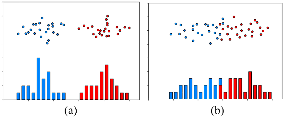
Illustration of Fisher scores with high one in (a) and low one in (b).

Subsequently, the most two high-score features are selected as training data for the algorithm.

Normalization

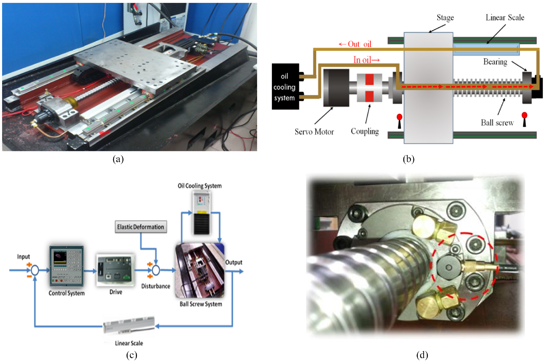
In this step, data are scaled to the same order using normalization to reduce the computation complexity. The formula is shown in equation (10).

X_{s} = \frac{x_{i} - x_{\min}}{x_{\max} - x_{\min}}

(11)

$x_{i}$ represents the i-th original data point, and $x_{\min}$ and $x_{\max}$ are the minimal and maximal value of the data, respectively, of the original data. $X_{s}$ is the data after normalization. The value of the normalized data is between 0 and 1. The value can be +1 to avoid computational errors in the exponential function or logarithm of the algorithm.

Experiment setup and results

Experimental design

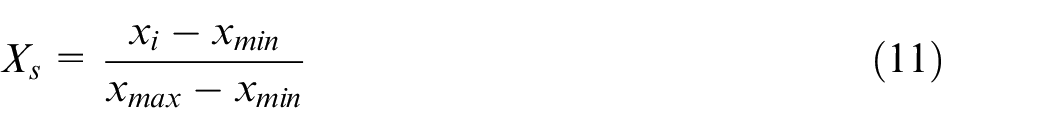
The machine employed for this research is shown in Figure 7(a). It was fabricated according to one axis of an industrial standard for a tapping machine. It had a 2-kW and 3000-rpm servo motor (Delta Electronics, Taiwan); an oil-cooling system shown in Figure 7(b) of 3 ψ and 220 V, with an accuracy of ±2°C; a mechanical structure accuracy of 5 μm, with a repeated accuracy of 2 μm; a maximum positioning speed of 48 m/min, with an acceleration of 1× g when the motor speed was 3000 rpm; and a sampling frequency of 8 kHz for data acquisition from the motor driver. The table was set for a traveling distance of 270 mm with reciprocating movement by varying the motor speed from 300 rpm to 900 rpm, with or without oil-cooling circulation and 20-kg payload conditions. The table was driven by a servomotor, followed by a coupler and a single-nut hollow ball screw (Hiwin R-36-16(K3)-FSC-C1-527-855-0.006-H) with various ball-nut preload and pretension levels. The standard ball-screw preload force was determined to be 4% of its maximum dynamic force of 3750 kgf. The maximum static force of the ball-screw preload was 9542 kgf. In this study, the preload percentage of the maximum dynamic force was divided into three categories: 2%, 4%, and 6%. Oversized balls were used in the single-nut ball screw to provide various preload statuses. The speed, acceleration, and S curve were controlled with a CNC controller (LNC-M310i-V) with feedback from a Heidenhain© encoder strip. Figure 7(c) presents the control block diagram for this single axis system, while 7(d) illustrates the attached accelerator sensor for detecting the vibration.

Figure 7.

Picture of the in-house single-axis hollow ball screw platform with a servo motor and linear scale positioning sensor (a), the illustration for the oil cooling circulation for the hollow ball screw (b), the block diagram for the experimental control system, and the attached accelerator near the ball nut.

In this study, the 4% preload was treated as the standard preload for typical precision motion in industrial applications. Therefore, a 2% preload indicates a preload loss situation, increased mechanical backlash, increased pitted ball trace, low stiffness, and oscillatory position errors. Moreover, the pretension and oil-cooling system on the hollow ball screw were used to achieve thermal rigidity compensation for improving the positioning accuracy.

The first phase of this experiment involved identifying the most useful built-in signal for classification. We employed a single-axis ball screw to do a back-and-forth motion which is shown in Figure 8, and acquired built-in data from internal parameters such as position, motor current, and revolution. Then, Fisher’s criteria were employed to investigate the most discriminative data among the built-in data.

Figure 8.

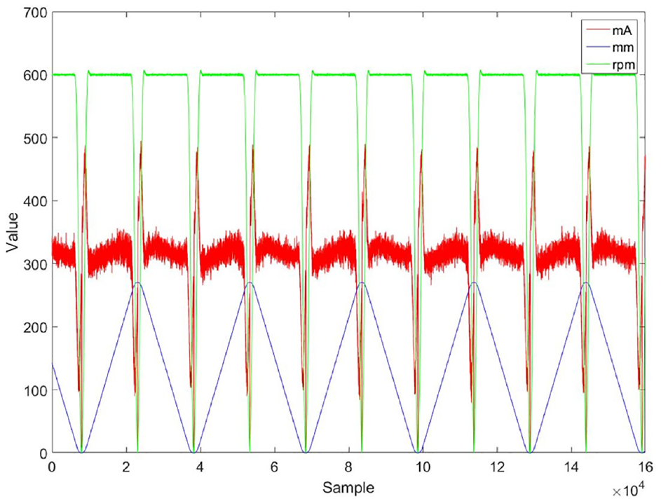
Current, positioning and associated rpm for a fixed reciprocation path.

After investigating the most useful built-in signal, we used the signal to conduct a follow-up study. The reciprocation path is too simple to satisfy the requirement of machining conditions in a realistic plant. As a result, we designed a path that is similar to the realistic path in a factory to reduce warm-up time efficiently. The current value of proposed process path is shown in Figure 9. We sought the best parameter σ and C in the SVM algorithm from the range of 2⁻⁵ to 2⁵.²⁴ The flow chart of this experiment is shown in Figure 10.

Figure 9.

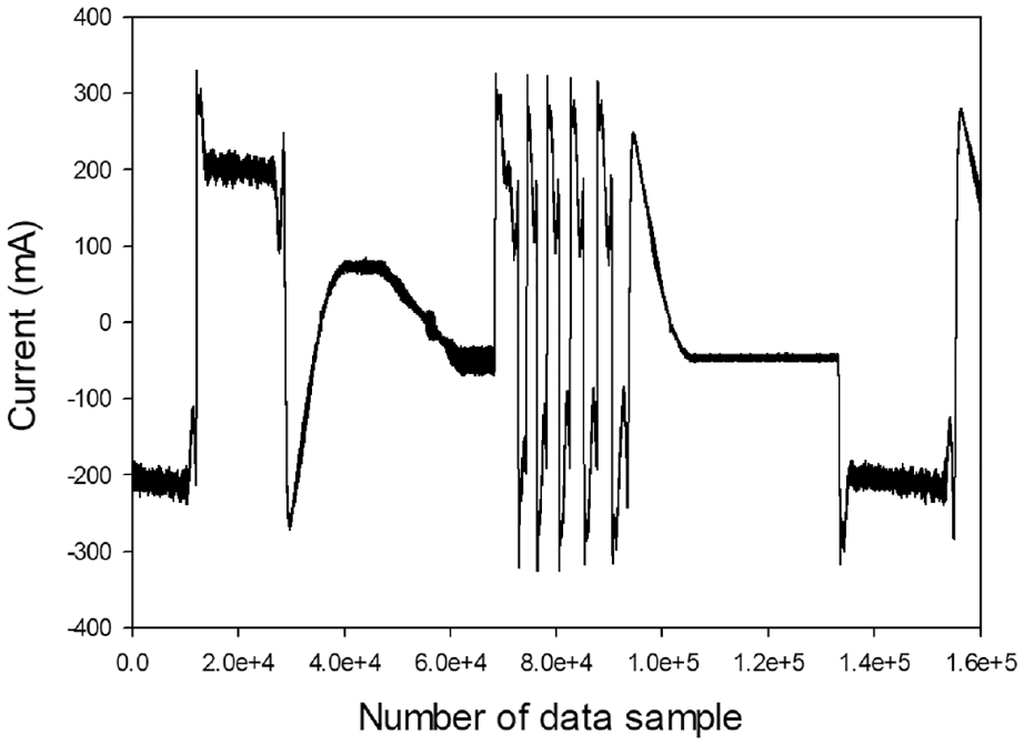
The current value of proposed process path for sampling 8 kHz based on 20 s of each commanded realistic path.

Figure 10.

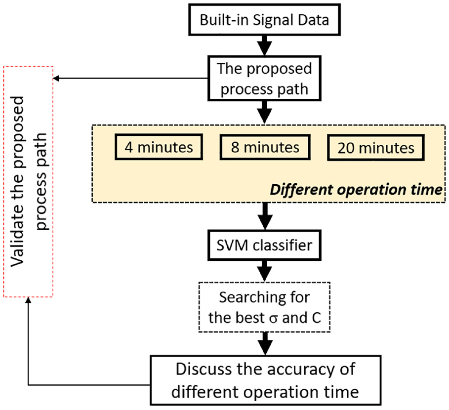
Flowchart of the experiment to validate the proposed process path.

However, each classification problem was in agreement with its best parameter C. It is extremely inefficient to investigate the C value of the SVM algorithm for every classification problem. As a result, we constructed a feature engineering to identify the discriminating features. Because the discriminating features of different classes were already perfectly separated, the value of C would not influence the results of the SVM classification.

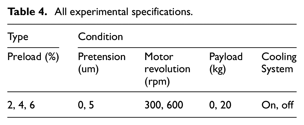
The raw feature engineering data are from the experiment detailed in the following section. The hollow ball screw reacted with the single-axis. The experimental conditions are shown in Table 4. During every test, one factor in type or condition served as the independent variable and the rest of the factors were control variables. The built-in signal was acquired for 2 min at 15-, 30-, and 60-min points during one operation. The sampling rate for these built-in signals was 8 kHz.

Table 4.

All experimental specifications.

Type	Condition
Preload (%)	Pretension(um)	Motorrevolution(rpm)	Payload(kg)	CoolingSystem
2, 4, 6	0, 5	300, 600	0, 20	On, off

The proposed method, feature engineering, was employed for raw data processing. The raw data served as the input of feature engineering, and the output of feature engineering was the most discriminative features. In this case, 144 experiments of preload diagnosis and 72 experiments each of pretension diagnosis, payload diagnosis, and cooling system diagnosis were conducted. The flow chart of the experiment to deploy the feature engineering is shown in Figure 11.

Figure 11.

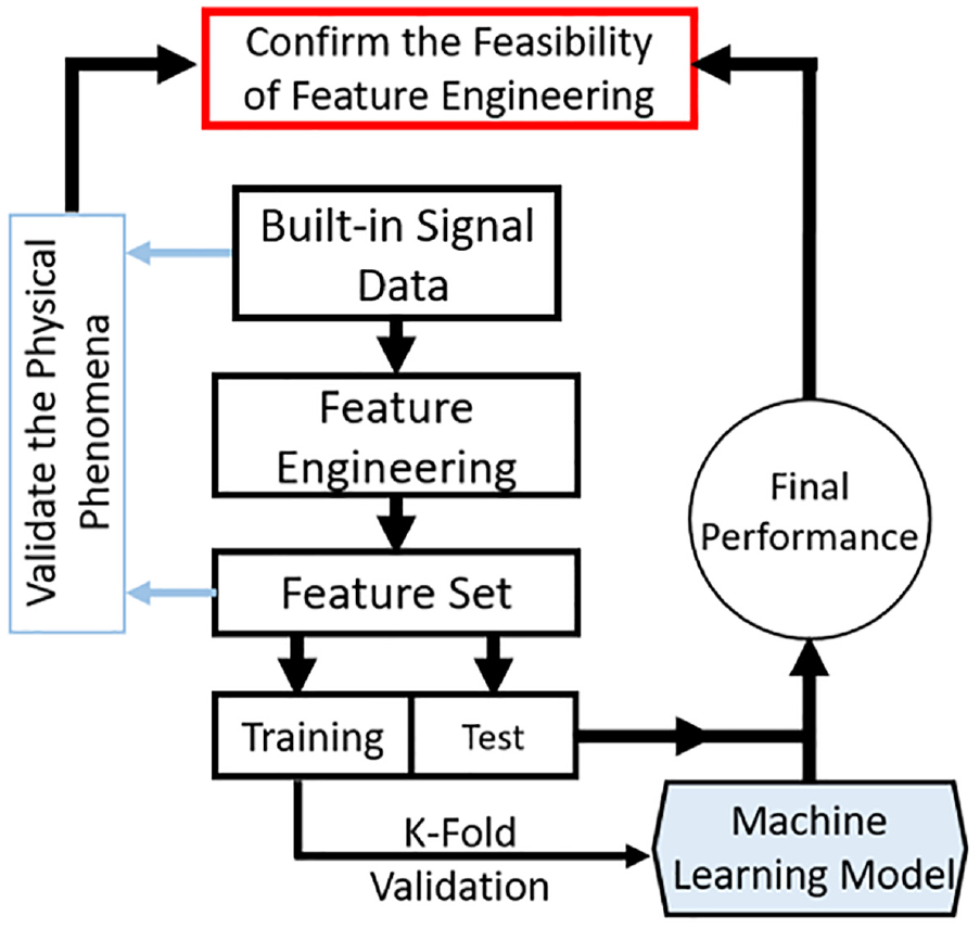
Flowchart of the experiment to validate the feature engineering.

Half of the experimental data set were trained and the rest of data set based on 5-fold validation was for testing.

However, not all signals were useful for classification. Some methods deal with imbalanced data set and feature selection is based on dynamic feature importance.^24,25 In this study, we employed Fisher’s criteria to seek and select the most useful signals for classification among the three built-in signals before the two aforementioned experiments were conducted.

Results and discussion

The aim of the first phase was to identify the most helpful-classified built-in signal from the acquisitioned current, position and motor’s rpm signals. All the results of the Fisher score experiments revealed the Fisher score for current signal was the highest one in Figure 12. In all experiments, the Fisher score for current was the highest among the three built-in signals at all times. This means that the current signal is the most useful built-in signal. The other two signals in terms of millimeter and revolutions-per-minute dimensions were partially overlapped with pretty low Fisher score. The result can also be observed in the outcome shown in Figure 12. Large ball screw preload gives the effect of frictional force and thermal deformation problem when the machine tool is in operation. Such effect causes the variation of the driving servo motor current. Calculated fisher scores represented the most discriminating acquisitioned signal for different preload types. Fisher score will be used for the comparison value of different preload types, for an example of 2% with 4% or 4% with 6%. The aforementioned score indicated that the current signal was the most useful built-in signal for classification. As a result, we used the current signal for diagnosis in the second phase. Figure 13 presents a result of a SVM classifier for 2% and 4% preload types directly with three built-in original signals without any feature engineering process. It was clear that the SVM resulted in a classification hyper surface from the perspective of current signal. This coincides with the result of Figure 12 that the current signal provides bettering classification solution for diagnosis.

Figure 12.

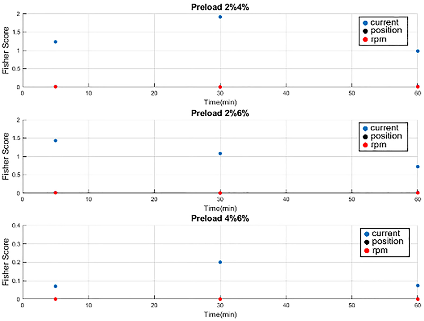
Plot of Fisher score for three built-in signals by three different operation time.

Figure 13.

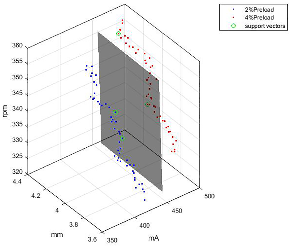
SVM classifier with three built-in signals.

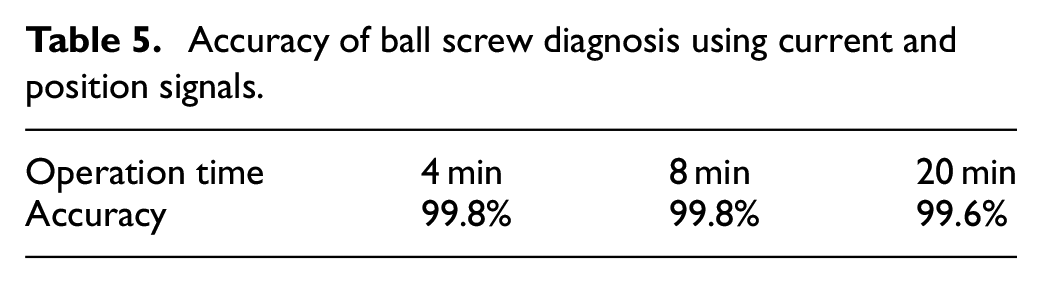
Although with long-term functioning, the preload and extent of ball screws is subject to thermal deformation, and the change of preload and the longitudinal pretension of ball screw lower the diagnostic performance. The results of our experiment to validate the robustness of the process we proposed are shown in Table 5. The accuracy is slightly changed from 99.8% to 99.6%. The results show that there is no severe effect on the diagnostic performance with a change in working time. That means the realistic manufacturing process path can be deployed to reduce the warm-up time.

Table 5.

Accuracy of ball screw diagnosis using current and position signals.

Operation time	4 min	8 min	20 min
Accuracy	99.8%	99.8%	99.6%

Next step is to select the two most discriminative features. Illustration of the Figure 14, the solid points represent training data and x points represent predicting data. The 2%, 4%, and 6% represent the preload; C and NC denote the opening and closing of the cooling system; 0 u and 5 u denote the pretension values; 300 rpm and 600 rpm represent motor revolution; and 5, 30, and 60 min are operation times in the diagram title.

Figure 14.

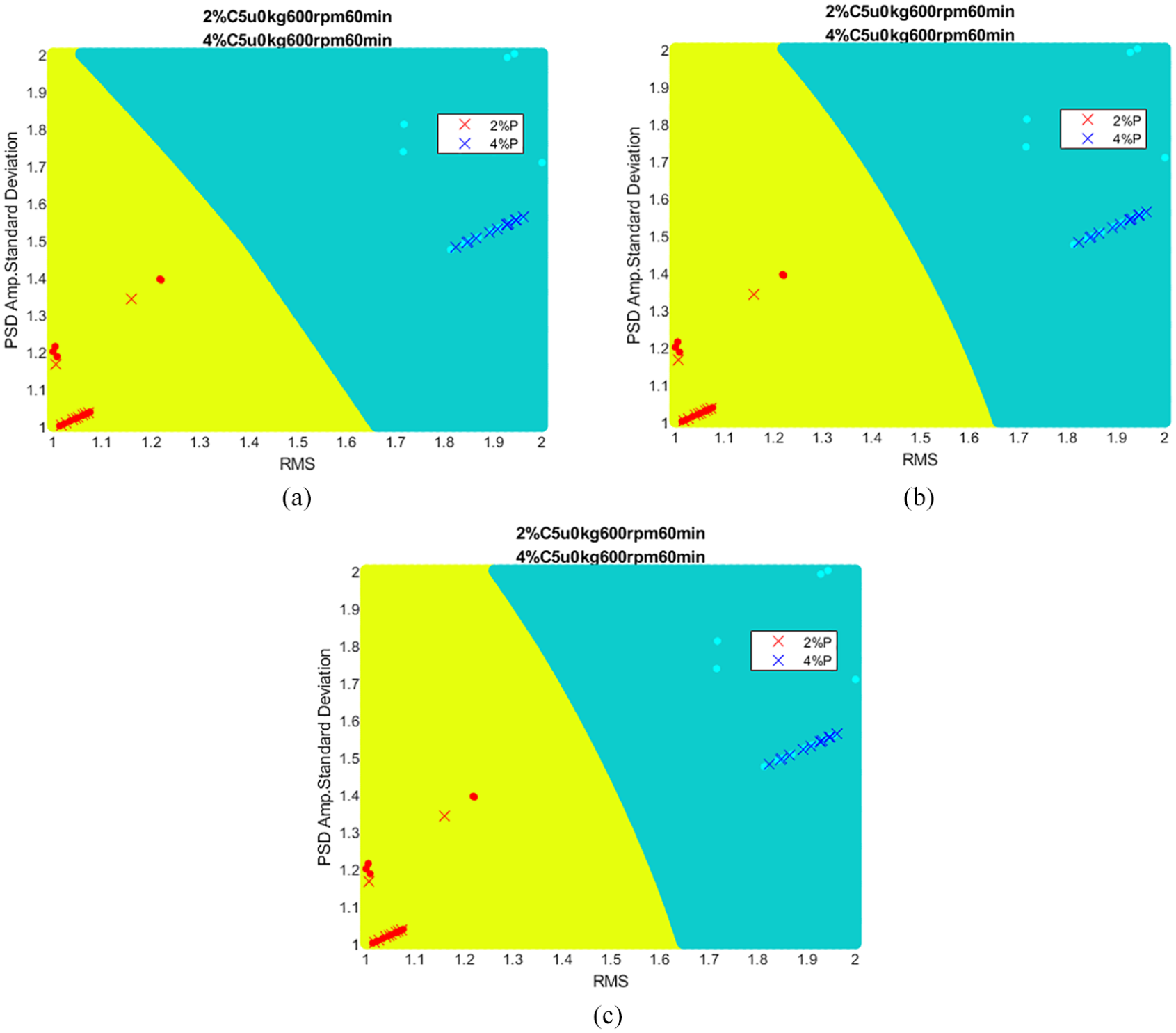
Results for different C values: (a) C = 0.1, (b) C = 1, and (c) C = 10.

Figure 14 conducted feature engineering first and established three C values for the SVM classifier.

We can observe that there was no critical effect on the variance of C values. Because the data processed by feature engineering were already distinguished, no misclassified data points were present. As a result, it was not challenging to identify the appropriate C value in this study.

Preload diagnosis

The Fisher score bar graphs of each type of preload diagnosis are shown in Figure 15. The red area represents the feature in time domain, as the number 1 to number 6 shown in Table 2. The green area represents the average amplitude of frequency in the frequency domain, as the number 7 to number 86 shown in Table 2. The yellow area represents the features in the frequency domain, as the number 87 to number 94 shown in Table 2. The x-axis shows the order-feature and the y-axis shows the average Fisher score of a certain diagnosis type.

Figure 15.

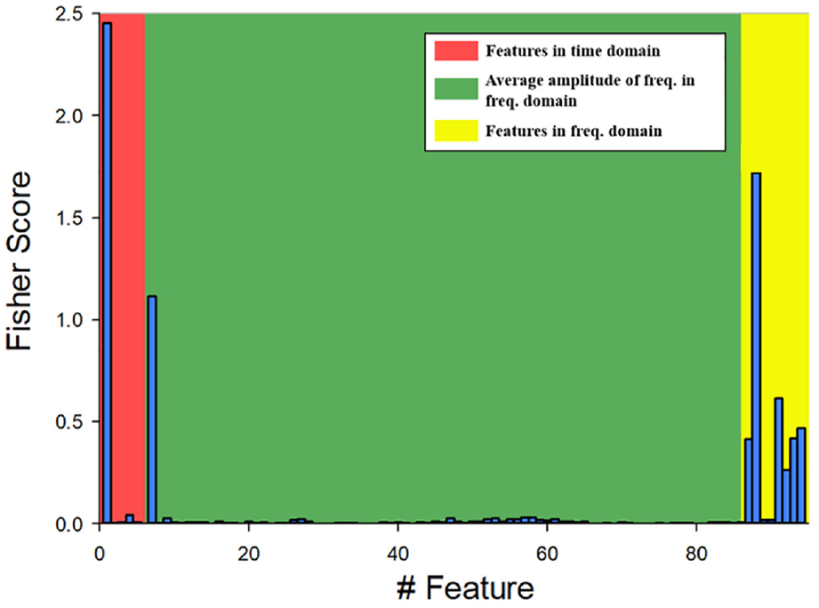
Fisher score bar graph for preload diagnosis.

Figure 15 demonstrated that RMS corresponded to the highest fisher score among the bar graph. The second highest score feature was PSD – amplitude standard deviation. In Figure 16(a), the top two fishers score features for the 2% and 4% preload diagnosis were RMS and PSD – Amplitude Standard deviation. The features of for the 2% and 6% were RMS and PSD – Shape Mean in Figure 16(b). According to results of the 144 preload experiments, there are 126 diagnosis experiments in which the RMS feature get into the top two fisher scores. That means the number of the RMS feature which is selected as one of the two most discriminating features is 126. As a result, the RMS feature is the most discriminative feature.

Figure 16.

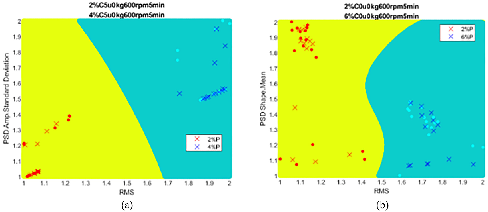
SVM classifier results for examples of two preload diagnosis.

From the perspective of RMS-dimension, the performance in discriminating the SVM features was excellent. The real-time waveform data are shown in Figure 17.

Figure 17.

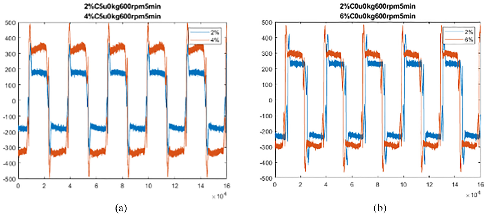
Real-time waveform in preload diagnosis.

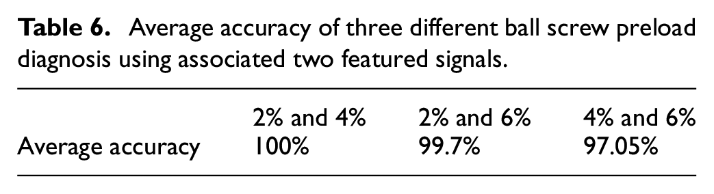
Because the two types of the waveform have been separated already, the RMS feature distinguished from all features and received the highest Fisher score. The reason for this phenomenon might be that the motor output different current because of the different normal forces the balls exerted on the screw. As a result, the two types of wave form is separable. The average accuracy of three different preload condition diagnosis is shown in Table 6. For an example, the diagnosis for two 2% and 4% preload tests of the total 144 experiments, the average accuracy (based on two different pretension conditions, on/off cooling oil, with/without payload, and two different rpm rotation) is 100%. Since the 4% preload stands for standard preload, while, the 2% stands for preload loss.

Table 6.

Average accuracy of three different ball screw preload diagnosis using associated two featured signals.

	2% and 4%	2% and 6%	4% and 6%
Average accuracy	100%	99.7%	97.05%

Pretension diagnosis

The Fisher score bar graph of the 72 experiments in the pretension diagnosis is illustrated in Figure 18. The feature with the highest score was RMS, and the feature with the second highest score was frequency domain. Favorable SVM classifier performance was achieved by training the features which get high fisher score. The SVM results are illustrated in Figure 19.

Figure 18.

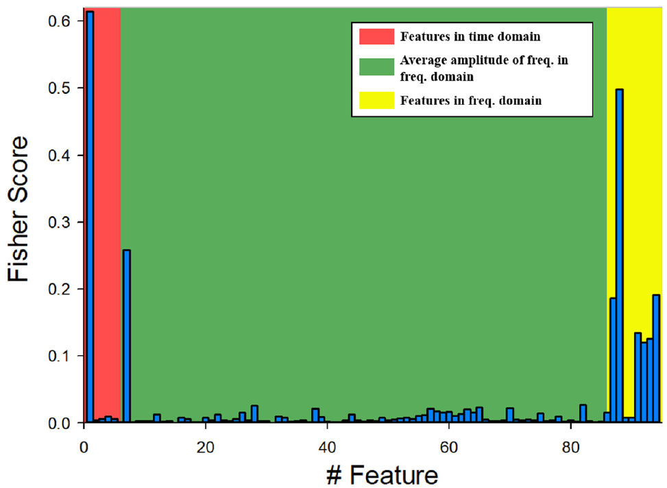
Fisher score bar graph for the pretension diagnosis.

Figure 19.

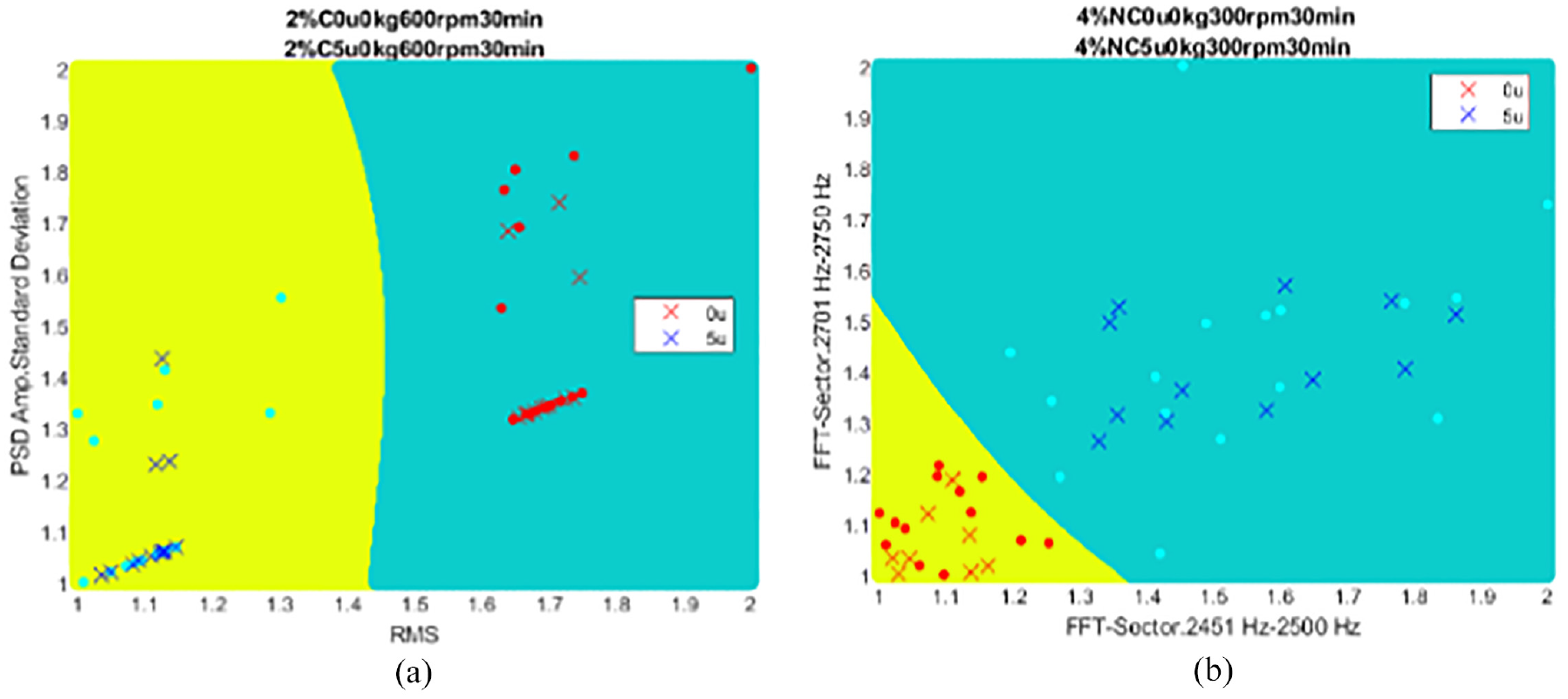
SVM classifier results for the pretension diagnosis.

In (a), in terms of RMS-dimension, the performance in discriminating the RMS feature was excellent. In (b), in terms of the FFT-Sector-dimension, the performance in discriminating of the FFT-Sector features was also excellent. Real-time waveforms are shown in Figure 20.

Figure 20.

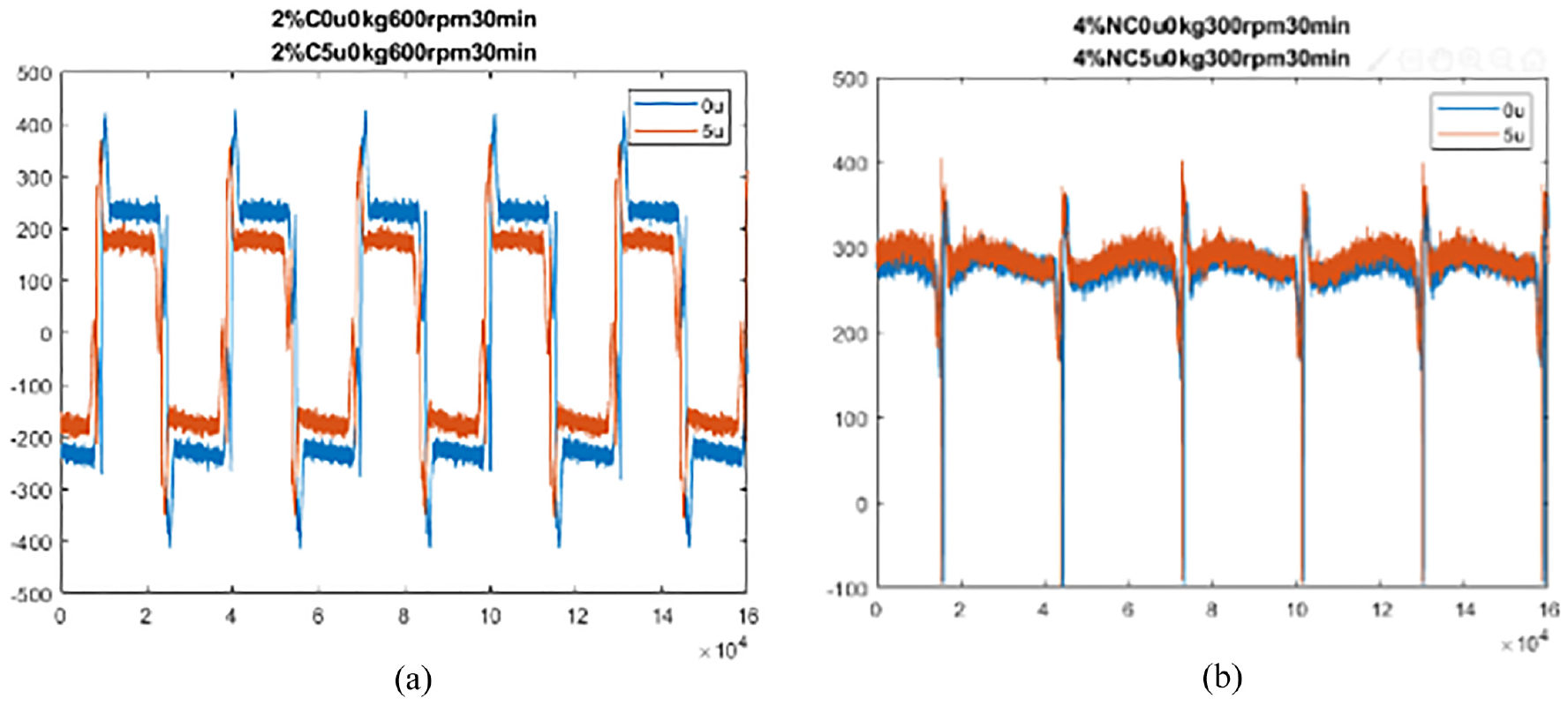
Real-time waveform for the pretension diagnosis.

The inference is similar to the inference for the preload diagnosis: the slightly different current output allows features in the frequency domain to be distinguished. As a result, these features are discriminated and obtain a high Fisher score.

Cooling system diagnosis

The Fisher score bar graph of the 72 experiments for cooling system diagnosis is presented in Figure 21. The diagnostic results for the cooling system were divided into pretension values of 0 μ and 5 μ. The results are illustrated in Figure 22. (A) is the ball screw with 0 μ in the cooling system diagnosis and (b) is the ball screw with 5 μ in said diagnosis.

Figure 21.

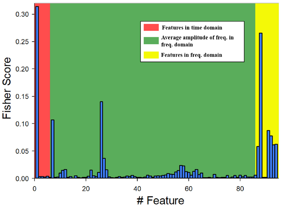
Bar graph of Fisher scores for the cooling system diagnosis.

Figure 22.

Bar graph of Fisher scores for the cooling system diagnosis with a 0-μ screw and 5-μc screw.

We divided the result of the cooling system diagnosis into two groups, those for 0 μm and 5 μm, and the accuracy levels of the two were 93.33% and 90.05% respectively. Screw pretension can inhibit thermal deformation; therefore, the influence of thermal deformation is greater for screws without pretension and SVM can classify them excellently. This phenomenon is illustrated in Figure 18. Because of the 5-μ screw’s capacity to inhibit thermal deformation, the variance of motor current is slight with long-term processing. As a result, the average amplitude of the frequency feature (the green area in Figure 22) corresponds to a higher score.

Moreover, in the 0-µm pretension cooling system diagnosis, dividing the results in 5, 30, and 60 min revealed accuracies of 90.56%, 93.32%, and 96.12%, respectively. The longer the operation time was, the higher the accuracy was. This was because the 0-µm pretension screw has a lower capacity to inhibit thermal deformation. As a result, the difference between opening and closing the cooling system is distinguished, and the SVM performance is high.

Payload diagnosis

The Fisher score bar graph for the 72 payload diagnosis experiments is presented in Figure 23.

Figure 23.

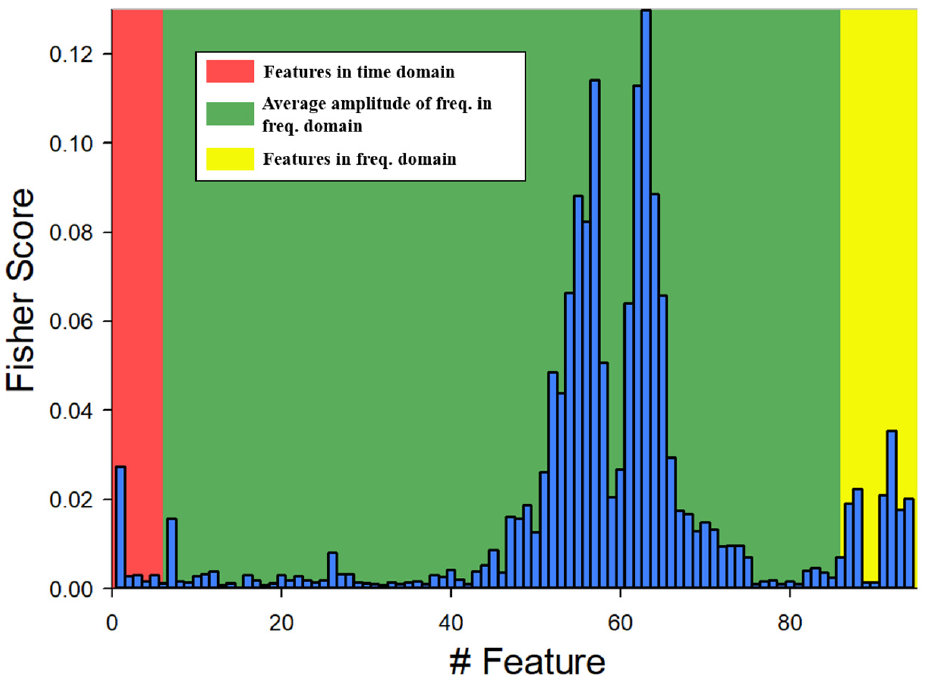
Fisher score bar graph for the payload diagnosis experiments.

According to results of the 72 payload diagnosis experiments, there are 68 experiments in which the FFT-Sectors features get the top 2 fisher score. That means, the number of the feature, FFT-Sectors, which is selected as one of the two most discriminating features is 68. The trend can be observed in Figure 23. The scores for the features in the frequency domain (the green and yellow areas) are higher than those for the features in the time domain (the red area). This shows that the features in the frequency domain are have more discriminative power than the features in the time domain. The SVM results are illustrated in Figure 24.

Figure 24.

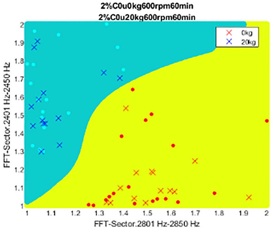
SVM classifier results for the payload diagnosis.

In terms of FFT-Sector-dimension, the performance levels related to discrimination of the FFT-Sector features were excellent. The real-time waveform data are shown in Figure 25.

Figure 25.

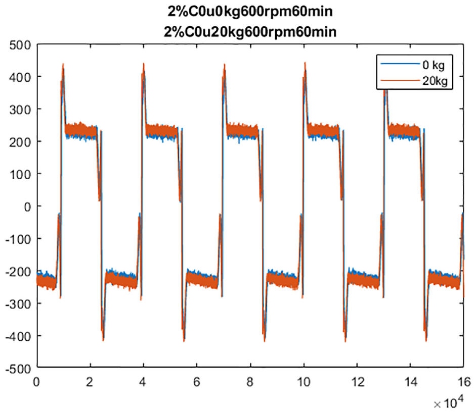
Real-time waveform for the payload diagnosis.

In the payload diagnosis, the two types of signals almost overlap. Moreover, no difference was noted between the two different motor current. This inference of this phenomenon is that the payload mass is undertaken by the linear guideway. As a result, the payload mass only slightly affects the real-time motor current and the features in the frequency domain have discriminative power.

Conclusions

A number of conclusions can be drawn from our study’s results. First, despite different signals in the time domain overlapping, feature engineering could still be employed to extract and select the most discriminative feature set for training the SVM algorithm, and its performance was favorable. Second, in the preload and pretension diagnosis, the different normal force and friction that the balls exerted on the screw caused different motor current outputs. For this reason, the preload and pretension diagnoses were simpler to classify than the cooling system and payload diagnoses were. Third, the operator can choose the RMS feature to train the classifier if the different waveforms are already separated. Fourth, 94 features were extracted in feature engineering, containing six time domain features and 88 frequency domain features. High Fisher scores were obtained for the frequency domain features, which benefits the performance of the classifier if the waveform overlaps in the time domain. Finally, in this study, the average accuracy of diagnosis for different conditions for ball screw preload, pretension, cooling system, and table weight were 98.91%, 94.08%, 91.69%, and 93.5%, respectively, after the feature engineering we constructed was used. This proposed architecture is validated by the experimental data and the accuracy of classification reaches successfully.

Footnotes

Declaration of conflicting interests

The author(s) declared no potential conflicts of interest with respect to the research, authorship, and/or publication of this article.

Funding

The author(s) disclosed receipt of the following financial support for the research, authorship, and/or publication of this article: This work was supported by MOST 108-2221-E-018-013, the authors are much appreciated.

ORCID iD

Yi-Cheng Huang

References

Wei

Lin

Horng

JH.

Analysis of a ball screw with a preload and lubrication. Tribol Int 2009; 42(11): 1816–1831.

Cuttino

Dow

Knight

Analytical and experimental identification of nonlinearities in a single-nut, preload ball screw. J Mech Des 1997; 119: 15–19.

Peng

Tse

Chu

FL.

A comparison study of improved hilbert–huang transform and wavelet transform: application to fault diagnosis for rolling bearing. Mech Syst Signal Process 2005; 19: 974–988.

Zhang

Zhou

, et al. Positioning error prediction and compensation of ball screw feed drive system with different mounting conditions. Proc IMechE, Part B: J Engineering Manufacture 2016; 230(12): 2307–2311.

Zhao

Zhang

YM.

Adaptive on-line compensation model on positioning error of ball screw feed drive systems used in computerized numerical controlled machine tools. Proc IMechE, Part B: J Engineering Manufacture 2019; 233(3): 914–926.

Wang

Vachtsevanos

Fault prognosis using dynamic wavelet neural networks. Artif Intell Eng Des Anal Manuf 2001; 15(4): 349–365.

Tsai

Cheng

Hwang

Ball screw preload loss detection using ball pass frequency. Mech Syst Signal Process 2014; 48(1–2): 77–91.

Bacha

Salem

Chaari

An improved combination of Hilbert and Park transforms for fault detection and identification in three-phase induction motors. Int J Electr power Energy Syst 2012; 43(1): 1006–1016.

Zheng

Zhang

, et al. Rolling element bearing fault detection using support vector machine with improved ant colony optimization. Measurement 2013; 46(8): 2726–2734.

10.

Wang

Zhang

Automatic blur type classification via ensemble SVM. Signal Process Image Commun 2019; 71: 24–35.

11.

Patel

Upadhyay

SH.

Comparison between artificial neural network and support vector method for a fault diagnostics in rolling element bearings. Procedia Eng 2016; 144: 390–397.

12.

Lee

Zhao

, et al. Prognostics and health management design for rotary machinery systems-Reviews, methodology and applications. Mech Syst Signal Process 2014; 42(1–2): 314–334.

13.

Fayyad

Piatetsky-Shapiro

Smyth

From data mining to knowledge discovery in data base. AI Mag 1996; 17(3): 37–54.

14.

Bedworth

O’Brien

The Omnibus model: a new model of data fusion?

IEEE Aerosp Electron Syst Mag 2000; 15(4): 30–36.

15.

Dasarathy

BV.

Sensor fusion potential exploitation-innovative architectures and illustrative applications. Proc IEEE 1997; 85(1): 24–38.

16.

Qiu

Lee

Feature fusion and degradation detection using self-organizing map. In: Proceedings of the 2004 international conference on machine learning and applications, Louisville, KY, USA, 16–18 December 2004, pp. 107–114. IEEE Xplore

17.

Casoetto

Djurdjanovic

Mayor

, et al. Multisensor process performance assessment through use of autoregressive modeling and feature maps. J Manuf Syst 2003; 22(1): 64–72.

18.

Jin

Chen

Lee

Methodology for ball screw component health assessment and failure analysis. In: Proceedings of the ASME 2013 international manufacturing science and engineering conference collocated with the 41st North American manufacturing research conference, Madison, Wisconsin, USA, 10–14 June 2013, 2: Systems; Micro and Nano Technologies; Sustainable Manufacturing. V002T02A031. ASME. https://asmedigitalcollection.asme.org/MSEC/proceedings-abstract/MSEC2013/55461/V002T02A031/267662

19.

Cortes

Vapnik

Support-vector networks. Mach Learn 1995; 20(3): 273–297.

20.

Boser

Guyon

Vapnik

VN.

A training algorithm for optimal margin classifiers. In: Proceedings of the fifth annual workshop of computational learning theory, Pittsburgh, PA, 27–29 July 1992, vol. 5, pp.144–152. Pittsburgh, PA: ACM Press.

21.

Vapink

Levin

CY.

Measuring the VC-dimension of a learning machine. Neural Comput 1994; 6(5): 851–876.

22.

Gangsar

Tiwari

Comparative investigation of vibration and current monitoringfor prediction of mechanical and electrical faults in induction motor based on multiclass-support vector machine. Mech Syst Signal Process 2017; 94: 464–481.

23.

Bishop

Jordan

Kleinberg

, et al. Pattern recognition and machine learning. Berlin: Springer, 2006, pp.1–4.

24.

Wei

Zhao

Feng

, et al. A novel hybrid feature selection method based on dynamic feature importance. Appl Soft Comput 2020; 93: 106337.

25.

de Haro-García

Cerruela-García

García-Pedrajas

. Ensembles of feature selectors for dealing with class-imbalanced datasets: a proposal and comparative study. Inf Sci 2020; 540: 89–116.

Applying a support vector machine for hollow ball screw condition-based classification using feature extraction

Abstract

Keywords

Introduction

SVM method

Feature engineering method

Data segmentation

Feature extraction

Outlier reduction

Feature selection

Normalization

Experiment setup and results

Experimental design

Results and discussion

Preload diagnosis

Pretension diagnosis

Cooling system diagnosis

Payload diagnosis

Conclusions

Footnotes

Declaration of conflicting interests

Funding

ORCID iD

References