
Abstract
The Moving Least Squares (MLS) and Moving Total Least Squares (MTLS) method are widely used for approximating discrete data in many areas such as surface reconstruction. One of the disadvantages of MLS is that it only considers the random errors in the dependent variables. The MTLS method achieves a better fitting accuracy by taking into account the errors of both dependent and independent variables. However, both MLS and MTLS suffer from a low fitting accuracy when applied to the measurement data with outliers. In this work, an improved method named as α-MTLS method is proposed, which uses the Total Least Square (TLS) method based on singular value decomposition (SVD) to fit the nodes in the influence domain and introduces a geometric characteristic parameter α to associated with the abnormal degree of nodes. The generated fitting points are used to construct the parameter and quantify the abnormal degree of the nodes. The node with the largest parameter value is eliminated and the remaining nodes are used to determine the local coefficients. By trimming only one node per influence domain, multiple outliers of measurement data can be effectively handled. There is no need to set threshold values subjectively or assign weights which avoids the negative influence of manual operation. The performance of the improved method is demonstrated by numerical simulations and measurement experiment. It is shown that the α-MTLS method can effectively reduce the influence of the outliers and thus has higher fitting accuracy and greater robustness than that of the MLS and MTLS method.
Introduction
In the past decades, meshless method 1 has been developed into an effective numerical method because of its good characteristics. In the meshless methods, the formation of shape functions is the primary issue. Many kinds of construction methods have been researched, such as the MLS method and the Radial Basis Functions (RBF) method.2,3 In the above-mentioned methods, the MLS method is widely used and was imported by Lancaster and Salkauskas 4 for the surface construction with the corresponding error analysis being discussed.5,6 Different from the traditional Least Square (LS) method,7,8 the complete polynomial is not applied to establish the fitting function in the MLS method. It consists of a coefficient vector related to the independent variable and a complete polynomial basis function. At the same time, the influence domain is divided by the compact support weight function, and the weight of nodes is distributed in the whole parameter domain. Therefore, the curve and surface reconstruction of the MLS method have the property of local approximation. The MLS approximation has been extensively recorded in the document and applied to engineering fields by many scholars.9,10 It derived numbers of methods to solve practical engineering problems for which numerical calculation methods are not suitable,11–13 for example, interpolating element-free Galerkin (IEFG) method for three-dimensional potential problems proposed by Liu 14 and boundary-free element method proposed by Wang 15 .
The MLS method has the advantages of simple calculation, high accuracy and smoothness.16,17 However, the LS method is applied to determine the local approximation and it assumes that there are no errors in the independent variables, while the random errors always occur on all the variables. In the sense of the TLS method, it is more rational to determine the local approximations.18–20 The MTLS method provides a better choice for handling the random errors of all variables. 21 Due to the influence of external factors such as artificial or environmental disturbance, the outliers are inevitable in the measurement data in practical engineering problems, which deviates from measurement data in some way and results in the instability of the reconstruction accuracy.22–24 In this case, neither MLS nor MTLS method can achieve good fitting accuracy due to their sensitivity to the outliers.
Therefore, it is necessary to find a method to avoid the negative effect of these outliers on fitting results. At present, there are two main methods that are feasible and commonly used.25,26 One of the common methods is to eliminate the outliers by setting a threshold value, and then operate reconstruction using the remaining data samples.27–29 Nevertheless, the performance of this method greatly depends on the selection of threshold value, and it is difficult to select the appropriate threshold. Another method is to select an appropriate weight function and assign a smaller weight to the outlier to reduce its influence in the fitting process. 30 Nevertheless, how to accurately determine the small weight and reduce the negative impact of the outlier is a thorny problem, particularly when there are multiple outliers. In addition, it is also unknown whether assigning small weights will have other negative effects or not. 31
To avoid the influence of outliers on the fitting accuracy, this paper presents an improved MTLS approximation named α-MTLS method. In the influence domain of this proposed method, the TLS method applying SVD 32 is used to fit the nodes. The generated fitting points are then applied to quantify the abnormal degree of nodes according to the geometric characteristic parameter α. By trimming only one node per influence domain, multiple outliers of measurement data can be effectively handled. This paper is structured as follows. Section 2 gives a brief introduction to the MLS method. Section 3 outlines the basic concepts of MTLS, and introduces in detail the proposed α-MTLS method. In section 4, the fitting performance of α-MTLS method is demonstrated by numerical simulations and experimental measurement compared with MLS and MTLS method. Finally, section 5 draws the conclusion.
MLS method
MLS is a well-developed method and can approximate the measurement data with high accuracy. The MLS approximation of a given function u h (x) is expressed as 33
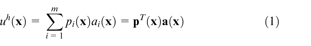
in which pi(
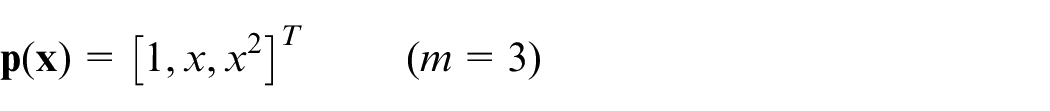
The commonly used basis functions in the two-dimensional case are described as follows.
Linear basis function:

Quadratic basis function:
To evaluate the approximation of the function, the coefficient
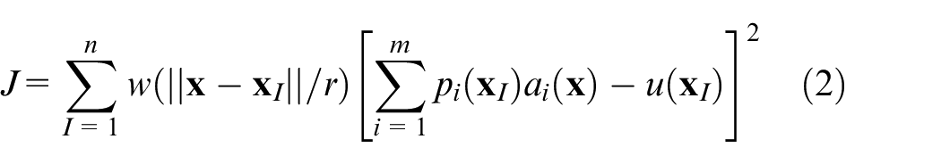
where w(||
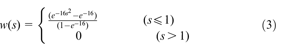
This exponential weight function divides the influence domain with
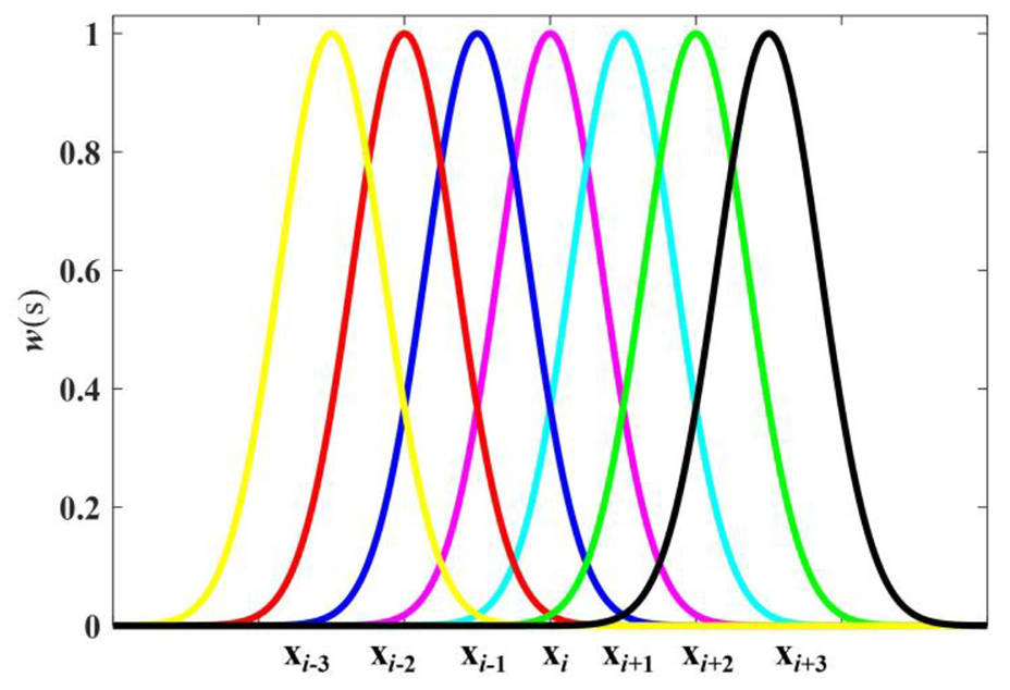
Diagram of the exponential weight function.
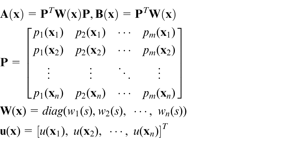
The values of the coefficients at the estimate points are acquired as below

where
The approximate function can be further expressed as

α-MTLS method
The classical MTLS method
The TLS method can be regarded as an advanced model of the least square method, which takes into account the interference of the regression matrix, whereas the influence of this factor is not considered in the general LS method. The error equation is expressed by

where
The SVD of C is expressed as 35

where singular matrix
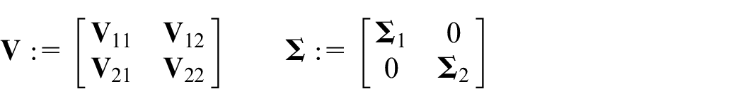
When

To determine the coefficients of local approximants, TLS method is applied to the influence domain of MTLS method. The matrix can be expressed as

where

MTLS method introduces TLS to determine local fitting parameters and takes the sum of squares of orthogonal residuals as the reference index, which is more rational in dealing with the errors of all variables, exactly as expressed in Figure 2.
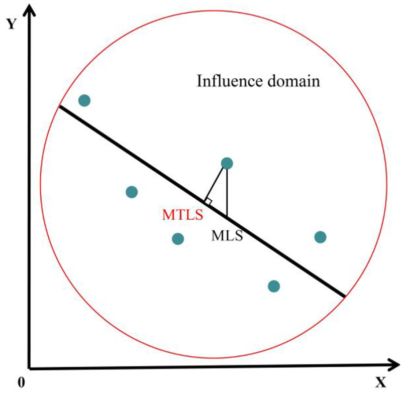
The approximation principle of MTLS method.
α-MTLS method
It can be seen from the above, the local approximants of MTLS method are executed in the orthogonal direction, in which the TLS estimations of influence domain are more appropriate for handling the errors-in-variables (EIV) model compared with the MLS method. However, the fitting accuracies of both methods do not meet the requirements when the outliers exist. Therefore, the α-MTLS is proposed to enhance the fitting accuracy and robustness when there are outliers in measurement data. The construction process of geometric characteristic parameter α for evaluating the abnormal degree of node is shown in Figure 3.
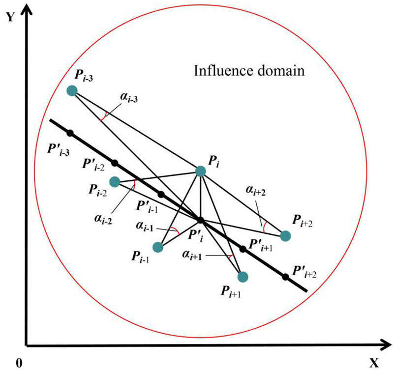
The construction process of parameter α
As shown in Figure 3, TLS method applying SVD is firstly used to fit the nodes Pi (i = i–3:i+2) in the influence domain to obtain the approximation line and generates the fitting points P′ i (i = i–3:i+2) which is in the approximation line and has the same xi with the corresponding node. The parameter α of Pi is the sum of angles formed by the fitting point P′ i and other nodes. For example, the angle αi–3 is formed by the line PiPi–3 and P′iPi–3, and the angle αi–2 is formed by the line PiPi–2 and P′iPi–2, and so on. It is apparent that N nodes can form N–1 angles and each node has one α value. The node with the largest α will be trimmed and the weighted TLS method applying SVD is employed to calculate the local coefficients using the remaining nodes. With the movement of the influence domain, the global reconstruction of the measurement data is completed in the whole parameter domain.
It can be seen from the introduction above that this method eliminates only one point in each influence domain and each eliminating process is independent of each other. To some extent, the parameter α of the node can reflect the deviation degree from the approximation line and can be used to evaluate the abnormal degree of each node. Different from the MTLS method, in the influence domain of α-MTLS method, the abnormal degree of the generated fitting point is quantified according to the geometric characteristic parameter α, and the outliers will be eliminated.
The following flowchart in Figure 4 shows the procedure of the improved method.
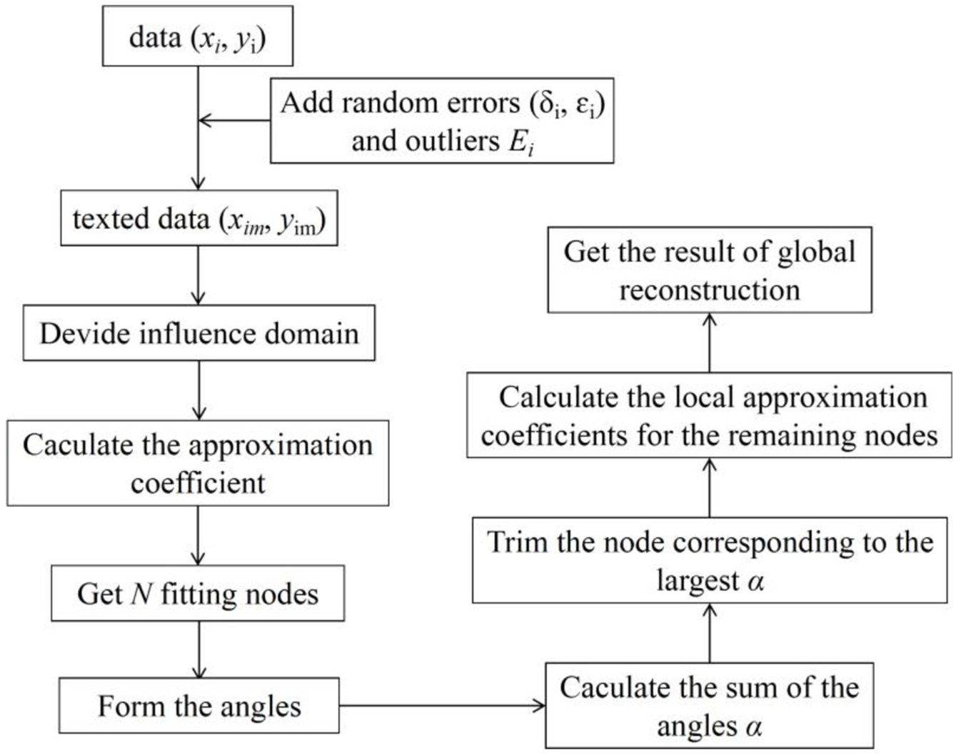
The procedure of the α-MTLS method.
Numerical and experimental examples
Numerical simulations and experimental examples are given to validate the performance of the α-MTLS method. The fitting results obtained by the MLS and MTLS method are shown as well for comparison.
Case 1
Within this example, the aspheric profile function is considered

where c = 1/1025 is the curvature of the base circle and k = –1.2 is a constant. A set of evenly distributed points (xi, yi), i = 1, 2, …, n obtained by equation (11) are selected and random errors with a mean value of 0 and normal distribution (δi,
The fitting accuracy can be evaluated by the sum of the differences between the theoretical values and the fitting values as well as the Root Mean Square (RMS) value
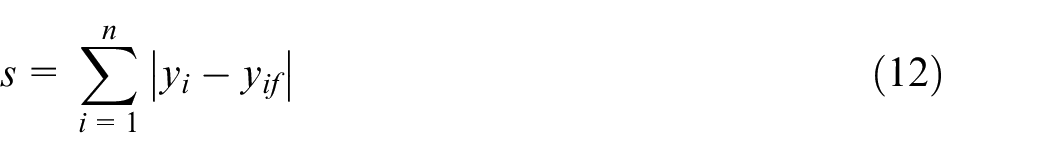
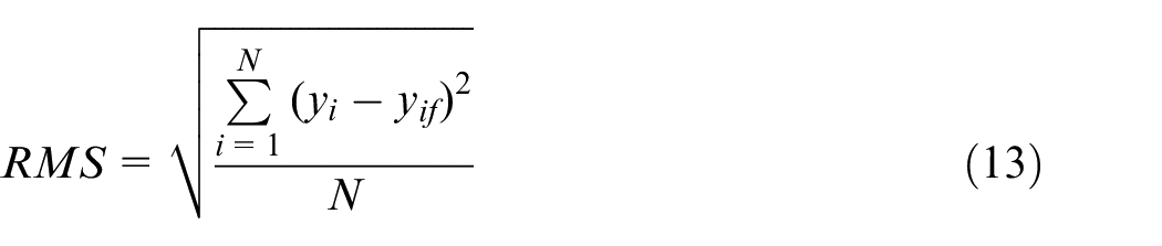
where yi is the theoretical value and yif is the fitting value.
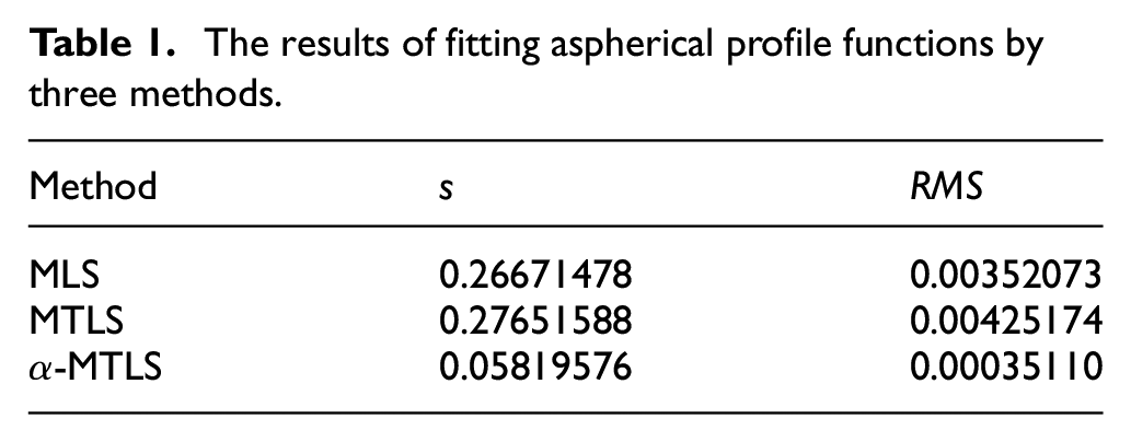
Let n = 121 and d = (max(x)–min(x)) × 1/10, where max(x) = 30 and min(x) = 0. The simulated data is fitted by MLS, MTLS and α-MTLS method respectively. Figure 5 shows the fitting curves of the three methods and the corresponding sum of differences and RMS values for the methods above are listed in Table 1.
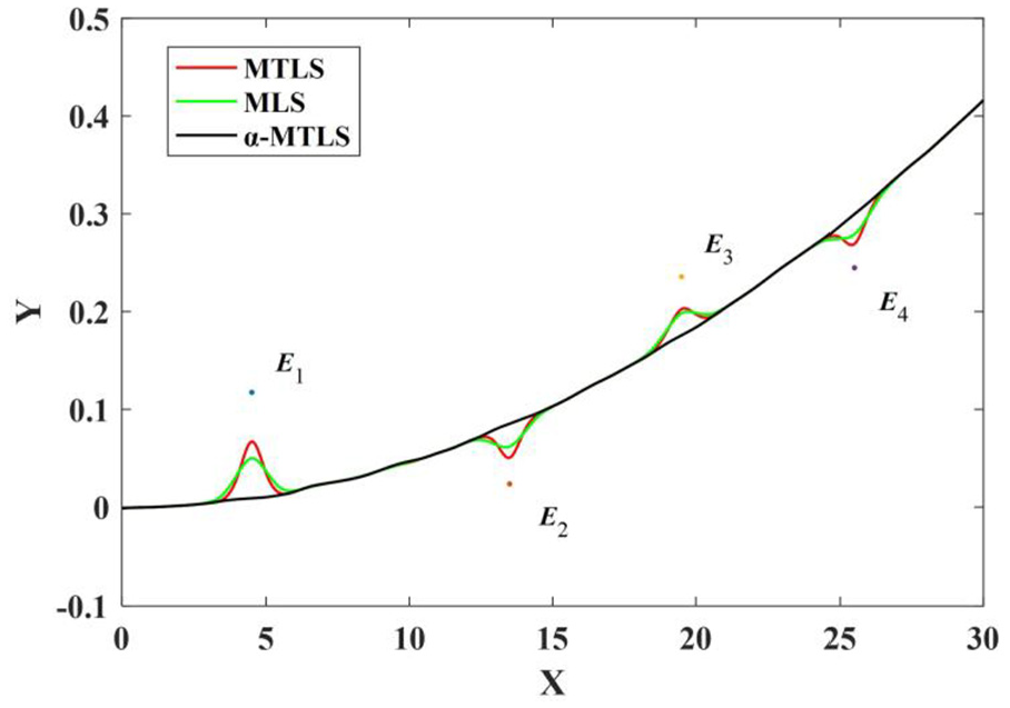
The aspheric curve fitting by three methods.
The results of fitting aspherical profile functions by three methods.
Case 2
The wave function is investigated

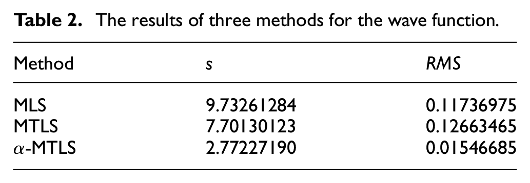
Under the conditions of n = 201 and d = (max(x)–min(x)) × 1/10, in which max(x) = 1 and min(x) = −1. The data is acquired using the same method as that described in Case 1 and is processed by MLS, MTLS and α-MTLS method separately. The corresponding sum of differences and RMS values are shown in Table 2 and the fitting curves are plotted in Figure 6.
The results of three methods for the wave function.
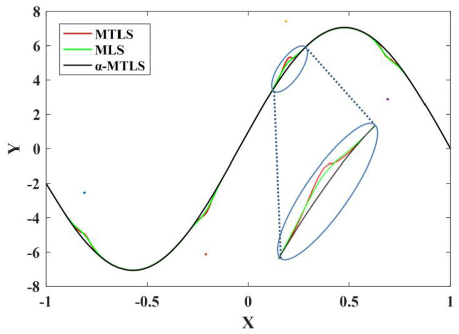
The wave curve fitting by MLS, MTLS and α-MTLS.
As shown in Figures 5 and 6, the existence of outliers greatly affects the fitting accuracy of MLS and MTLS methods, which makes the nearby data deviate from the normal nodes. Meanwhile, Tables 1 and 2 also show that even if there are only a few outliers in the global domain, the reconstruction result will be totally different. Obviously, the proposed α-MTLS method can achieve a better fitting result for the data with outliers in terms of accuracy and robustness.
Case 3
Within this example, the three-dimensional discrete data of the function are considered
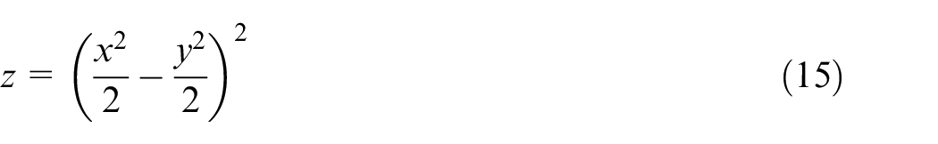
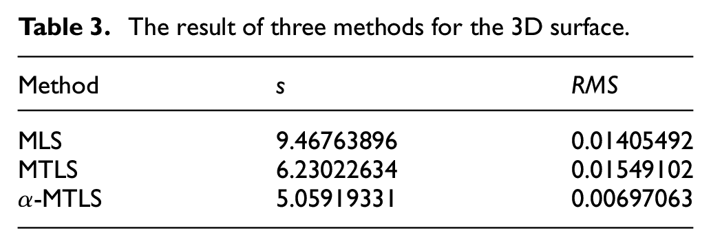
the domain Ω is assumed as Ω = [–1, 1] × [ –1, 1] and the surface is divided into a mesh of 33 × 33 nodes. The case is carried out under the conditions of n = 1089 and d = (max(x)+max(y))/10, where max(x) = 1 and max(y) = 1. The fitting results by MLS, MTLS and α-MTLS are shown in Table 3 and Figure 7.
The result of three methods for the 3D surface.
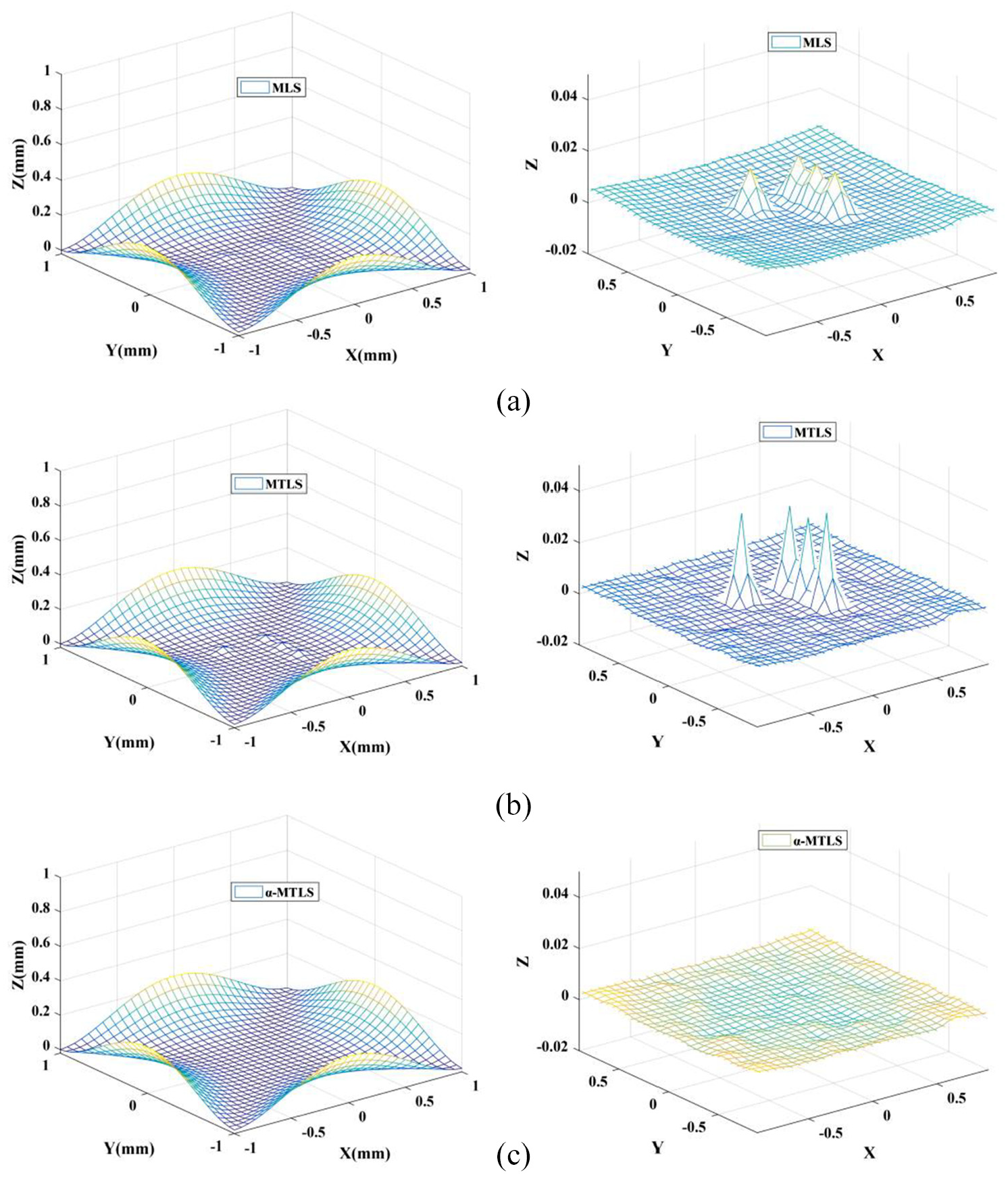
The surface fitting by three methods. (a) The fitting and error surface of the MLS method. (b) The fitting and error surface of the MTLS method. (c) The fitting and error surface of α-MTLS method.
For the result of each method in Figure 7, the fitted surface and error surface are displayed on the left and right, respectively. It can be seen that although the MLS and MTLS method has good approximation character and can well reflect the geometric contour of the data, they are greatly sensitive to the outliers and only a few outliers in curves and surfaces will lead to the unstable reconstruction of a series of adjacent nodes. The proposed method can effectively eliminate outliers without affecting the reconstruction of nearby nodes and achieve a stable reconstruction accuracy.
Case 4
In this example, the experimental measurement data is used to validate the performance of the proposed method.
The measurement system is mainly composed of a mobile platform and a laser displacement sensor system. SILVERA 080 series guideway with precision positioning controlled by YASKAWA servo driver are used in the three-coordinate mobile platform system. The signal exchange between the mobile platform and PC is controlled by the control card Parker 1505. The feedback of motion position of each axis is provided by the RH 100 series grating displacement sensor produced by Renishaw. The other hardware includes digital display rotary table, electronic control cabinet, PC and so on.
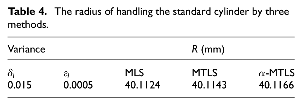
As shown in Figures 8 and 9, a non-contact displacement sensor KEYENCE LK-G150 is used to measure the horizontally fixed cylinder and acquire the contour data of the standard cylinder. The radius of the standard cylinder is 40.1840 mm calibrated by Taylor Hobson PGI 1240 profilometer. The contour data are fitted by MLS, MTLS and α-MTLS respectively. The reconstructed data are processed by the circle regression algorithm and thus the regression radii of three methods are obtained in Table 4. Figure 10 shows the fitting curve of the α-MTLS method. From the radius values in Table 4, compared with the other two methods, it can be known that the α-MTLS result is closest to the standard cylindrical radius under the same condition. The experimental result verifies the good performance of our proposed method.
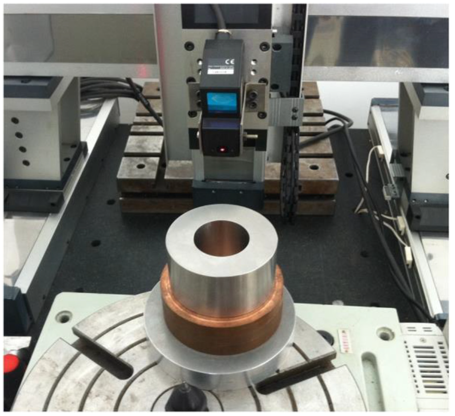
Experiment of measuring cylinder with CMM.
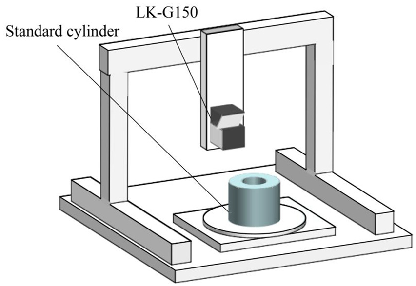
Schematic diagram of CMM.
The radius of handling the standard cylinder by three methods.
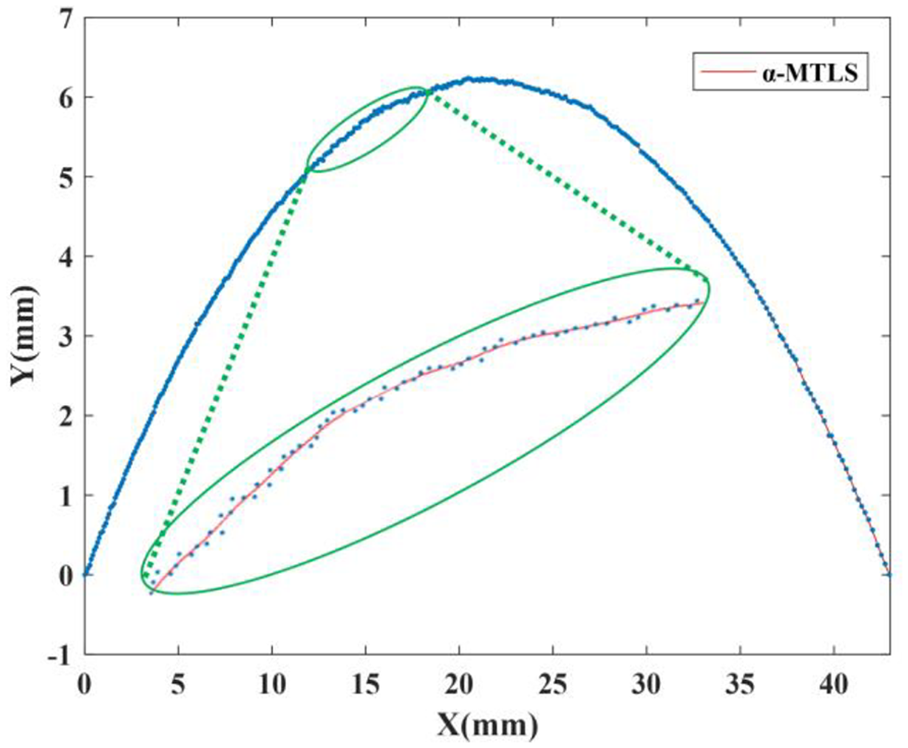
The profile fitting of standard cylinder by α-MTLS method.
As mentioned above, the errors in the measurement data are not seriously deviated, and the α-MTLS method still has better fitting accuracy. The case studies in this section demonstrate that α-MTLS method can eliminate the negative effect of outliers without human intervention. Only one node is trimmed per influence domain, even if there are several outliers, this method can also ensure fitting accuracy and robustness.
Conclusion
In this paper, a novel α-MTLS method is proposed, which avoids the negative effects caused by setting threshold value or allocating weights subjectively. In addition to its own characteristics, the α-MTLS method makes full use of all the advantages of the MTLS method. The shape function with high order continuity can be obtained by choosing suitable compact support function with low order basis function. In each influence domain of α-MTLS method, the abnormal degree of the generated fitting point is quantified according to the geometric characteristic parameter α, and the outliers will be eliminated. Numerical simulations and experimental measurement verify the effectiveness of the method.
Footnotes
Declaration of conflicting interests
The author(s) declared no potential conflicts of interest with respect to the research, authorship, and/or publication of this article.
Funding
The author(s) disclosed receipt of the following financial support for the research, authorship, and/or publication of this article: This work was supported by the National Science Foundation of China (Grant No. 11572316 and 51605094), the Fundamental Research Funds for the Central Universities (Grant No. WK2090050042), the Thousand Young Talents Program of China, and the Center for Micro and Nanoscale Research and Fabrication at the University of Science and Technology of China.