
Abstract
The moving least squares (MLS) and moving total least squares (MTLS) are two of the most popular methods used for reconstructing measurement data, on account of their good local approximation accuracy. However, their reconstruction accuracy and robustness will be greatly reduced when there are outliers in measurement data. This article proposes an improved MTLS method (IMTLS), which introduces an improved random sample consensus (RANSAC) algorithm and a correction parameter in the support domain, to deal with the outliers and random errors. Based on the nodes within the support domain, firstly the improved RANSAC is used to generate a model for establishing the group of pre-interpolation and calculating the residual of each node. Subsequently, the abnormal degree of the node with the largest residual is evaluated by the correction parameter associated with the node residual and random errors. The node with certain abnormal degree will be eliminated and the remaining nodes are used to obtain the approximation coefficients. The correction parameter can be used for data reconstruction without insufficient or excessive elimination. The results of numerical simulation and measurement experiment show that the reconstruction accuracy and robustness of the IMTLS method is superior to the MLS and MTLS method.
Keywords
Introduction
After decades of development, the reconstruction algorithms for discrete data have played an essential role in many engineering and scientific fields, especially in error analysis and data processing. The conventional numerical methods, such as finite element method (FEM), interpolate or approximate the nodes through defining a mesh based on known nodes. 1 However, the accuracy of reconstruction will be greatly reduced and the fitting will even fail when the grid-based method is used to deal with large deformation and discontinuity problems. 2 In addition, the human-labor and time cost of generating meshes in complex-shaped domains are not satisfactory. While meshless methods use node-based approximation without mesh discretization, the efficiency and accuracy of data processing are, therefore, greatly improved. 3 In order to meet the development requirement of different fields, a multitude of meshless methods have been presented and applied, such as the element-free galerkin (EFG), 4 diffuse elements method (DEM), 5 and moving least squares (MLS).
Mclain 6 proposed the weighted least squares method. On this basis, Lancaster and Salkauskas 7 introduced the moving concept and proposed the MLS method in 1981. To this day, the MLS has become an important method for constructing shape function. Unlike the traditional least square method using complete polynomials, the shape function of the MLS is composed of a coefficient vector and a basis function vector, which can obtain higher continuity under the condition with low order basis function. 8 The introduction of the weight function with compact support makes the reconstructed curve or surface accurate and smooth, which has contributed to the wide application of the MLS in various fields. For example, the MLS is applied to solve elasticity problems, 9 the compressible Navier-Stokes, 10 Kuramoto-Sivashinsky, 11 and Burgers equation, 12 and estimate mathematical model based on discrete points. 13 Due to its good performance, the MLS method is often used in combination with other methods to construct shape function. In finite element analysis, the introduction of the MLS method enhances the shape function of the active element. 14 In the smoothed particle hydrodynamics (SPH), the MLS method was used to construct kernel functions to obtain higher consistency. 15
The MLS method obtains the local fitting coefficients through the weighted least squares (LS) 16 method in the support domain 17 based on the Gauss Markov error model, in which only the dependent variable contains errors. 18 The total least squares (TLS) 19 method is an estimation method based on the errors-in-variables (EIV) model. Unlike the Gauss Markov model, the errors of both independent variable and dependent variable are considered in the EIV model. 20 By replacing the LS estimation with the TLS estimation in the support domain, the MLS method is transformed into the moving total least squares (MTLS). 21
Nevertheless, due to the impact of factors, such as the disturbances in the measurement environment, the measurement data often contains outliers that seriously deviate from the actual value.22,23 The LS and TLS respectively used in the support domains of the MLS and MTLS method are not robust estimation methods.24,25 When there are outliers in the domain, larger deviations will exist in the fitted values around outliers. Many studies have been carried out to reduce the negative impact from the outliers, with the proposed robust algorithms dividing into two main forms. One is to select a subsample from the discrete points to obtain the regression coefficient.26,27 If the outlier is in the subsample, it will be automatically eliminated. However, this method may eliminate some of non-outliers, in which case the accuracy of approximation will be significantly affected. 28 The other type of algorithm is to identify outliers first and then weaken the influence of outliers by assigning weights to them. In this method, it is difficult to determine appropriate weights when multiple outliers with different levels exist in the discrete data.
In order to weaken the impact of outliers on reconstruction, we propose an improved MTLS (IMTLS) reconstruction method in this article. In the support domain, we deal with outliers by introducing an improved random sample consensus (RANSAC) and a correction parameter, and then the local approximation coefficients are obtained based on the TLS estimation. RANSAC is a robust model estimation algorithm, especially when measurement data contains high proportion of outliers. However, it has limitations in data fitting influencing its accuracy and stability. 29 Therefore, RANSAC algorithm needs to be improved to estimate a relatively reliable initial model. The correction parameter associated with the random error and the node residual is introduced to detect and eliminate abnormal node.
The rest of this article is structured as follows: the second section is a brief introduction to the MLS, MTLS, and RANSAC algorithm, the third section explains the principle and procedure of the proposed algorithm in detail, and the fourth part verifies the performance of the IMTLS method through numerical simulation and experimental data.
Introduction to the basic algorithms
The MLS method
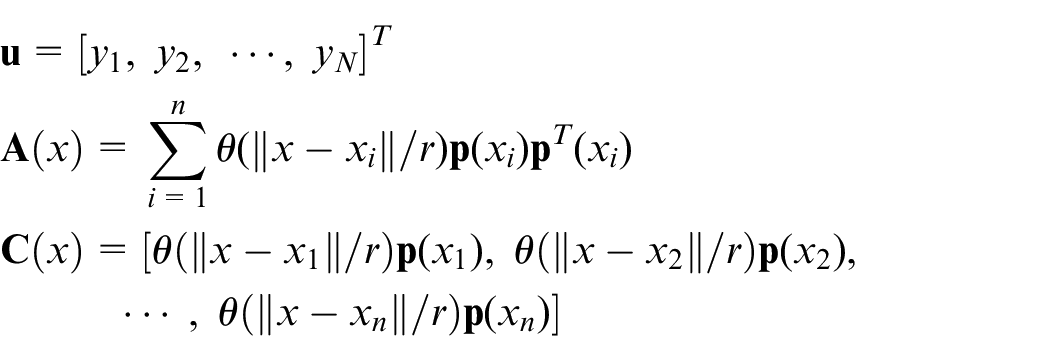
Consider that there are n discrete points
where
In order to solve the optimal
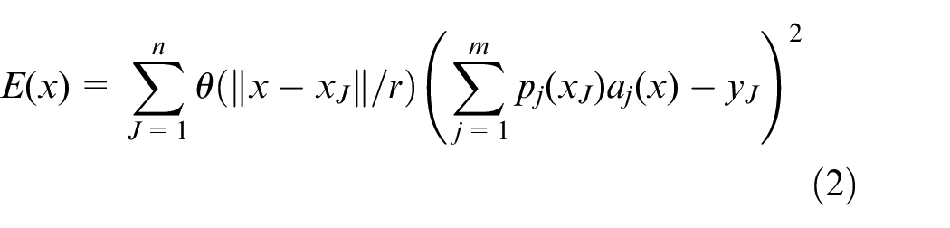
where r is used to control size of the support domain, and θ(||x–xJ||/r) is a non-negative and compactly supported weight function to attribute a weight to each node according to its position relative to x. The fitting property of MLS algorithm will be influenced by the weight function. For example, the fitting form will be interpolated when θ(0) = ∞. 30 There are many kinds of weight functions with compact support such as exponential, Gaussian, and cubic spline weight functions. This article chooses exponential weight function, that is,
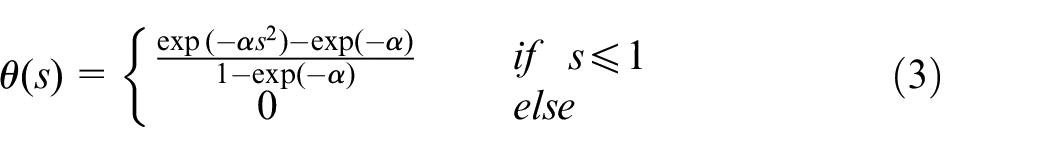
where α is a coefficient related to the convergence speed.
According to the principle of least squares, the coefficient vector
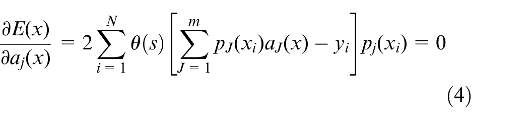
where j = 1, 2, …, m, solving equation (4) to obtain

where
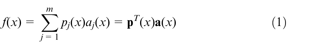
Taking equation (5) into equation (1), the function f(x) can be presented as

The MTLS method
Unlike the MLS using LS estimation to obtain the local fitting coefficients, the MTLS method applies the TLS estimation for those coefficients, in which the errors of both dependent variable and independent variables can be considered. In TLS, the solution of linear equation is considered, that is,

where

where
Therefore,
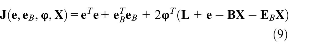
where
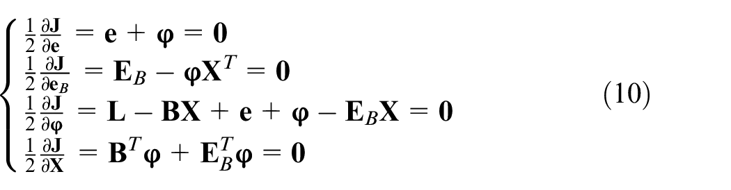
derived from equation (10), we can obtain
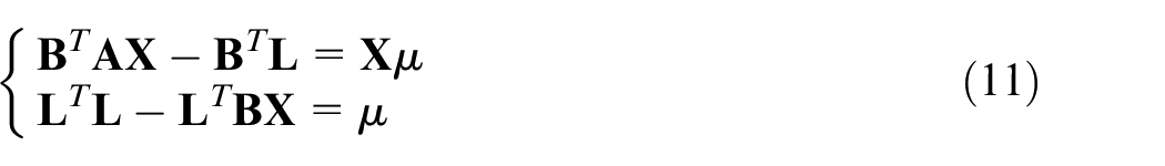
where μ =
The equation (11) can be transformed into
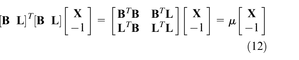
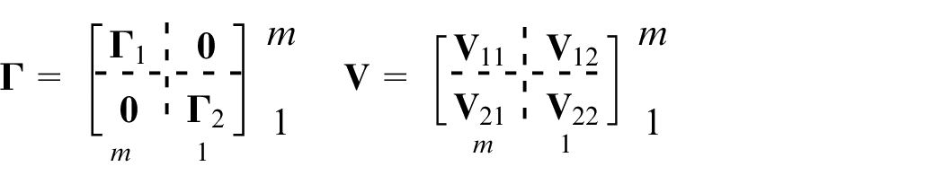
It can be seen from equation (12) that the problem of solving total least squares is transformed into obtaining the eigenvalues and eigenvectors of matrix [

where
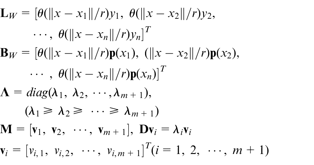
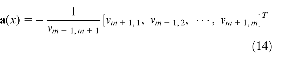
If λm+1≠λm, combined with equations (12) and (13), the regression coefficient vector
In the MLS method, the coefficient matrix
The RANSAC algorithm
The RANSAC algorithm, presented by Fischler and Bolles, 32 can robustly estimate the model parameters. It has been applied to many fields, especially in computer vision,33,34 due to good performance in handling the data with a tremendous level of outliers and remarkably simple structure. The main idea of the RANSAC is to calculate parameters of hypothesized model by randomly sampling the subsample from the entire dataset, 35 and then the model is performed on the entire dataset. During this process, a distance threshold that is considered empirically 36 is set to calculate the inlier rate of each model, and sampling is stopped when the number of iterations reaches the defined value. The parameters corresponding to the highest inlier rate (the highest consensus) are selected as the model parameters of the total sample. The brief calculation steps of the RANSAC algorithm are described as follows:
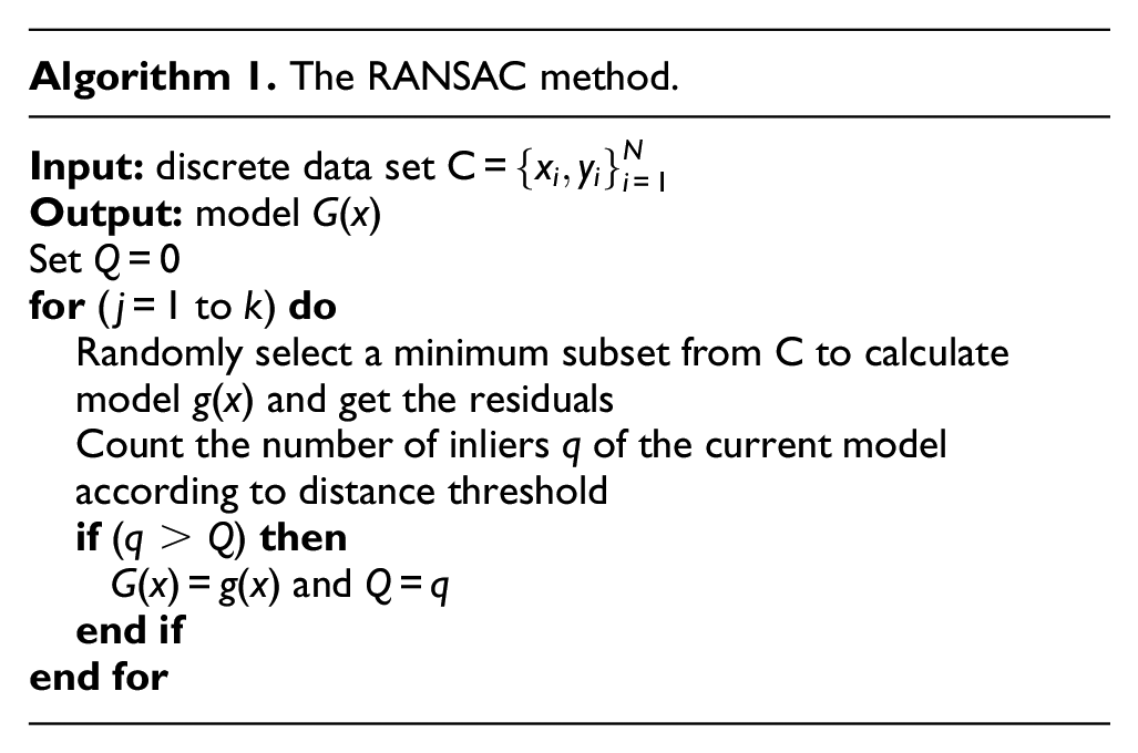
In order to get a subsample that is all inliers with probability p, the sampling times k can be obtained by the following formula, 37 that is,
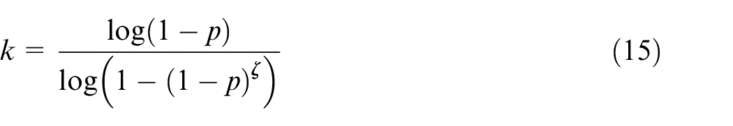
where w is the proportion of outliers in the entire dataset, and ζ is number of data nodes needed to calculate model parameters. For example, ζ = 2 is taken in the linear parameter estimation. Then a reliable model is obtained through multiple iterations, and the node with the residual outside the distance threshold is considered as outlier.
The improved MTLS method
When there are outliers in the measurement data, the robustness and accuracy of both the MLS and MTLS method are not satisfactory due to their construction principles. 38 Therefore, this article proposes an IMTLS method to reduce the negative impact of outliers on reconstruction. In this method, an improved RANSAC and a correction parameter are introduced into the support domain of the MTLS method to detect and eliminate abnormal nodes, and then the local fitting coefficients based on the TLS estimation can be obtained. The improved RANSAC algorithm is different from the standard RANSAC algorithm in two aspects. Firstly, it considers every possible subsample to generate hypothesized models, which can enhance the stability of data reconstruction. Secondly, the threshold is automatically set to a value related to the random error of the data, which reduces the negative impact of the original method to set a threshold empirically.
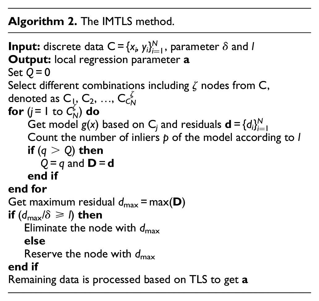
Then, we mainly introduce the principle and procedure of the algorithm reconstruction in support domain, as shown in Figure 1. Assuming that there are N nodes in single support domain, the reconstruction process of the MTLS method can mainly be divided into three steps. Firstly, an estimation model is obtained by the improved RANSAC algorithm. Secondly, the abnormal node is eliminated by introducing a correction parameter δ. In this step, whether to eliminate the node with the largest residual is determined by the size of dmax/δ and l, where dmax is the maximum residual and l is automatically set according to the random error of the data. Lastly, local approximation coefficients are determined by TLS estimation. In the support domain, the calculation process of the IMTLS method is shown as follows:
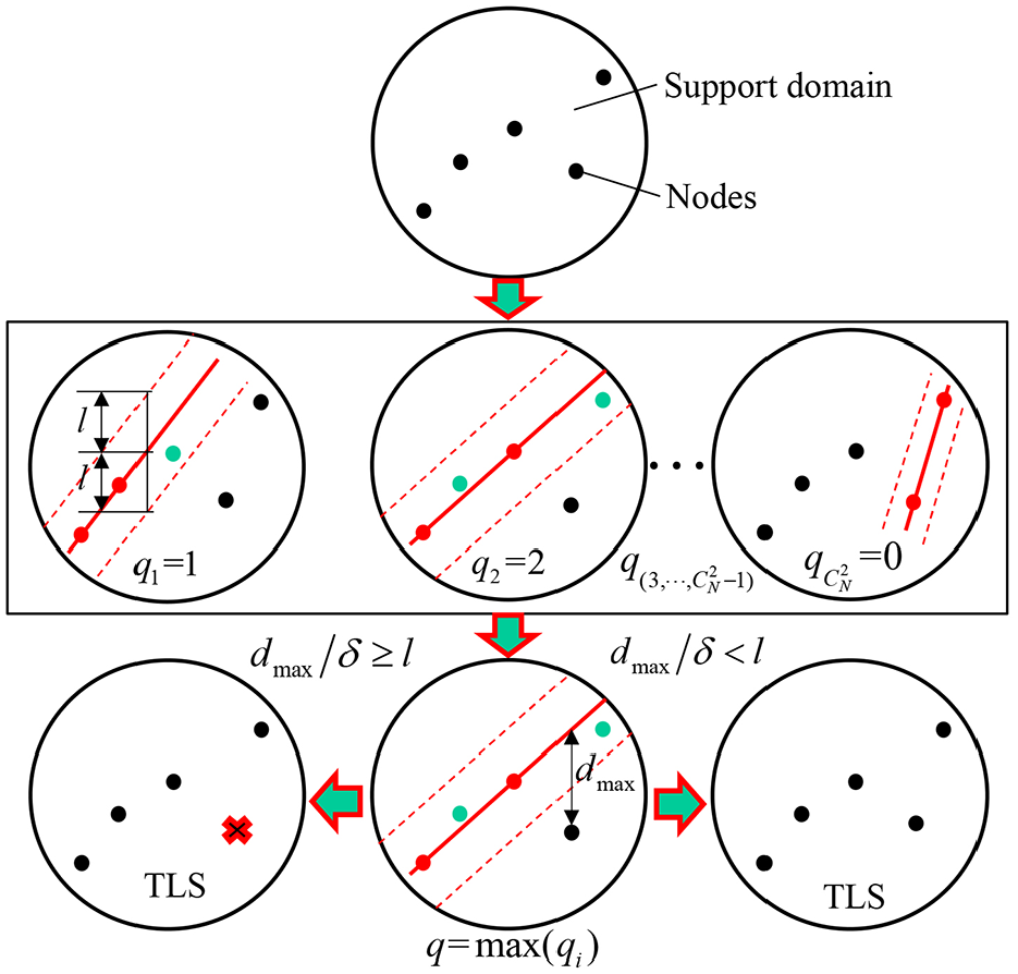
The fitting procedure in the support domain of IMTLS method.
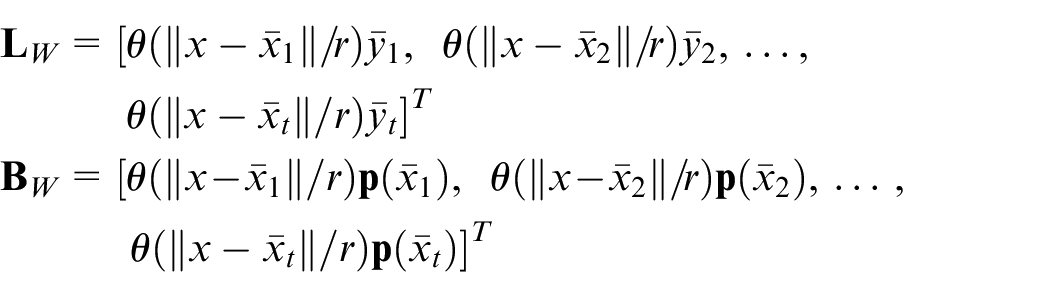
After eliminating the abnormal nodes, assume that t nodes
in which
When

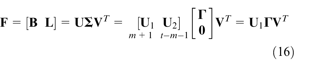
For the IMTLS method, the matrix

Where
The solution expression of equation (17) is rewritten as

In the support domain of the IMTLS method, abnormal nodes are automatically detected and eliminated by the improved RANSAC method and the introduced correction parameter δ. The outliers are evidently included in the abnormal node and can be effectively processed. The local fitting coefficients are obtained by the TLS estimation. As the movement of fitting point x, outliers and random errors are processed in the entire domain.
Case verification
In this section, both numerical and experimental cases were considered by the MLS, MTLS, and IMTLS method, to verify the performance of the proposed method.
Case 1
Take the curve function

as a model to generate uniformly distributed discrete points (x0i, y0i). Outliers (0, Δyi) and random errors of normal distribution with zero mean are added to (x0i, y0i) to get simulation data (x1i, y1i). The reconstruction points (x2i, y2i) are obtained after reconstruction. The sum of absolute differences can be presented as
which is considered as the index to evaluate three algorithms.
In this case, the parameter
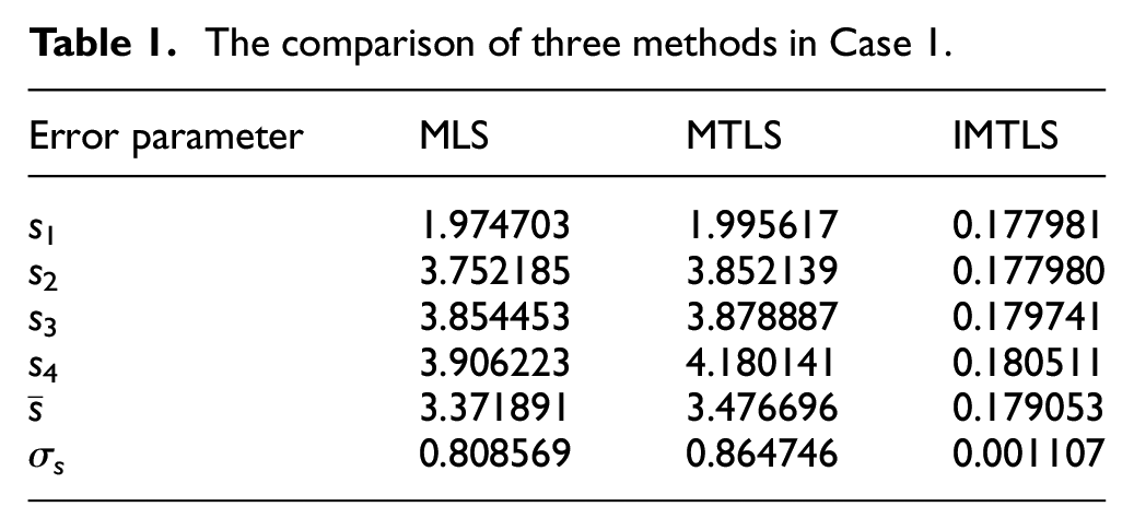
Let n = 201 and r = [max(x0)−min(x0)] × 4/100, where min(x0) = 0 and max(x0) = 5. Under the same random error condition (σx = 0.001 and σy = 0.001), we add four different outliers to (x0i, y0i), and the s values obtained by three algorithms are shown in Table 1. The fitting curves are shown in Figure 2.
The comparison of three methods in Case 1.
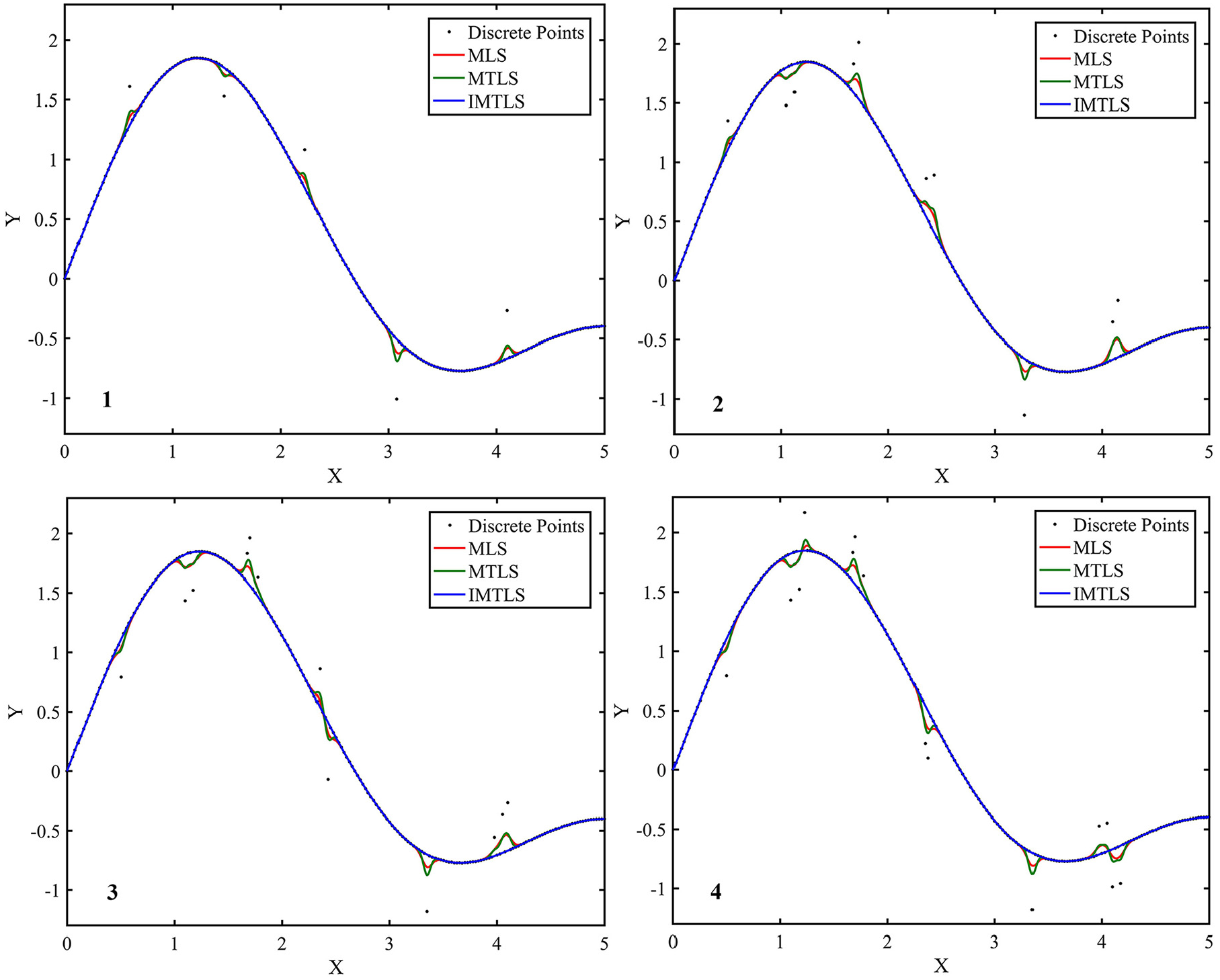
The curves fitting by three algorithms under different outlier conditions.
The figures and tables of the above cases show that outliers can be effectively detected and eliminated by the IMTLS method to reduce the incalculable negative impact on the reconstruction. Compared with the MLS and MTLS method, the error values of the reconstructed data processed by the IMTLS method is much smaller.
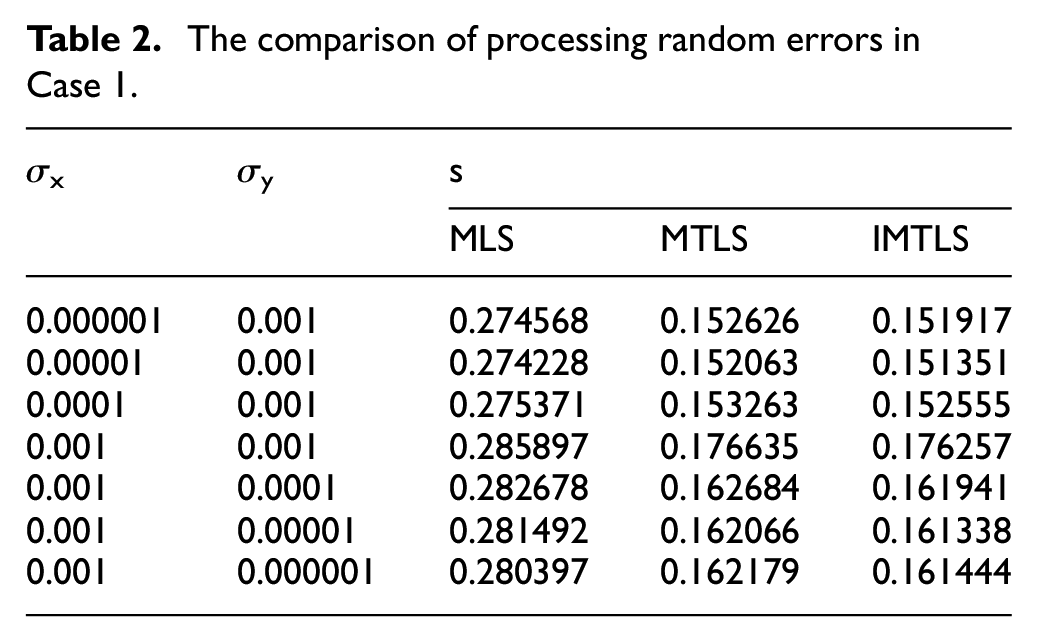
To further verify the performance of the IMTLS method, we take this case as an example, in which only random errors are added in the simulation data. In Table 2, we can see that the error values obtained by the IMTLS fitting is still minimum among the three reconstruction methods, which shows that the IMTLS method also has good approximation performance under this situation, and Figure 3 shows the bar graph of error values under different random errors.
The comparison of processing random errors in Case 1.
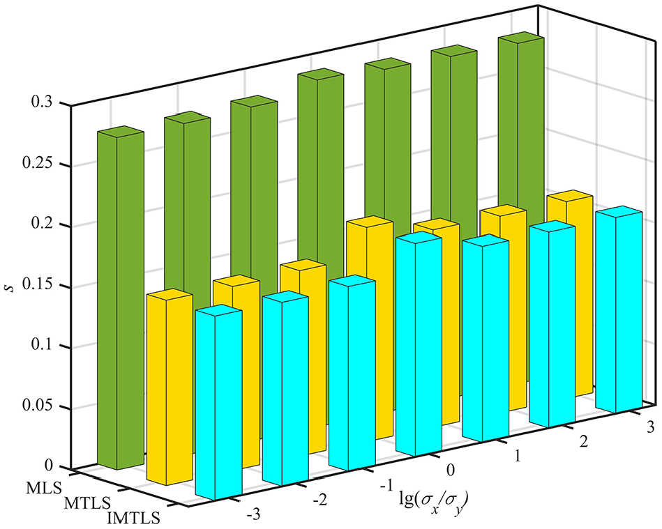
The s values under different random errors.
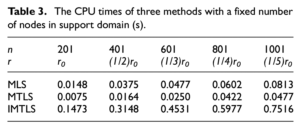
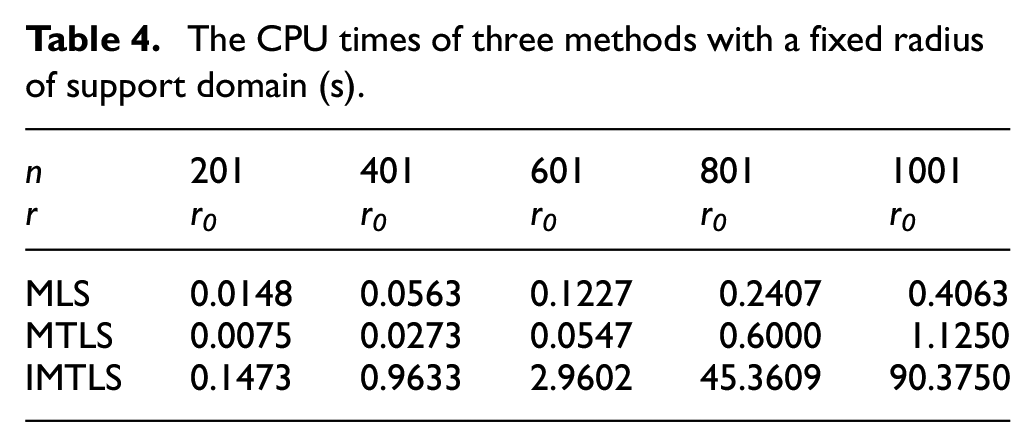
Furthermore, the CPU time of each algorithm is calculated by MATLAB based on the datasets with different size of n = 201 + i × 200 (i = 0, 1, …, 4). Two conditions are considered and presented in Tables 3 and 4 (r0 = [max(x0)−min(x0)] × 4/100, where max(x0) = 5 and min(x0) = 0) respectively. One is to fix the number of nodes in support domain, and the other one is to fix the size of support domain. In the first condition, CPU time of IMTLS method changes steadily with the increase of n. While in the second condition, the CPU time of IMTLS method increases rapidly as n increases because more nodes are included in single support domain. These results illustrate that the number of nodes in the support domain has a significant impact on the CPU time of IMTLS method. Therefore, in order to ensure the efficiency of IMTLS method in data reconstructing, the size of support domain should be appropriately selected to control the number of nodes in support domain.
The CPU times of three methods with a fixed number of nodes in support domain (s).
The CPU times of three methods with a fixed radius of support domain (s).
Case 2
In this case, the surface data of standard ball was processed to verify the performance of the IMTLS method. The data is obtained by a commercial white light interferometer (WLI) – Taylor Hobson CCI 3000.
Figure 4 shows the schematic diagram of a WLI system. Firstly, a broadband illumination beam passes through an interferometric objective via a beam splitter. The beams that were reflected by reference mirror and measured surface were focused onto a camera. Interference fringes will generate when the optical path difference (OPD) between the reference and measurement arm is within the coherence length, and the visibility of the fringes increases as OPD decreases. A series of interferograms can be obtained through scanning the objective. Surface data can be obtained by tracking all coherence peaks or phase retrieval within the field of view of the objective.
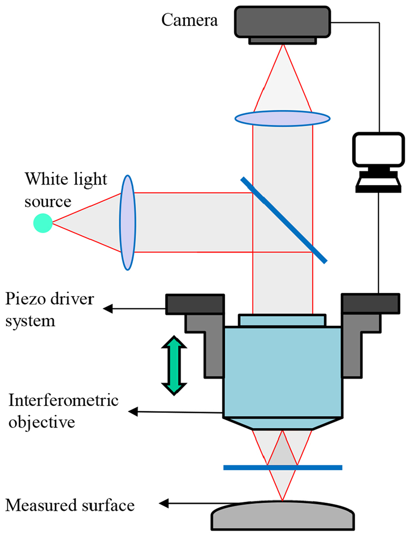
Schematic diagram of a WLI system.
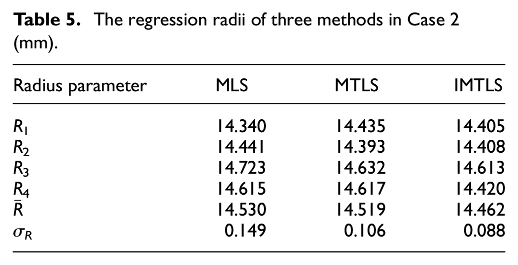
The errors contained in experimental data will have a negative impact on obtaining the true profile of the ball measured, and the impact can be reduced by using appropriate algorithm for reconstruction. Three methods are used to reconstruct the experimental data respectively. Then, the reconstructed data are used for parameter regression based on simulated annealing algorithm 40 and the regressed radius is used as the evaluation index of reconstruction method. The radius of standard ball is calibrated as 14.402 mm. Since the random error of measurement data cannot be calibrated technically, l is defined to the standard deviation of residuals fitted by the LS estimation in support domain. As shown in Figure 5, data selected in different locations are processed by three algorithms. As shown in Table 5, the radius corresponding to the IMTLS is more proximate to the calibrated value among the three algorithms.
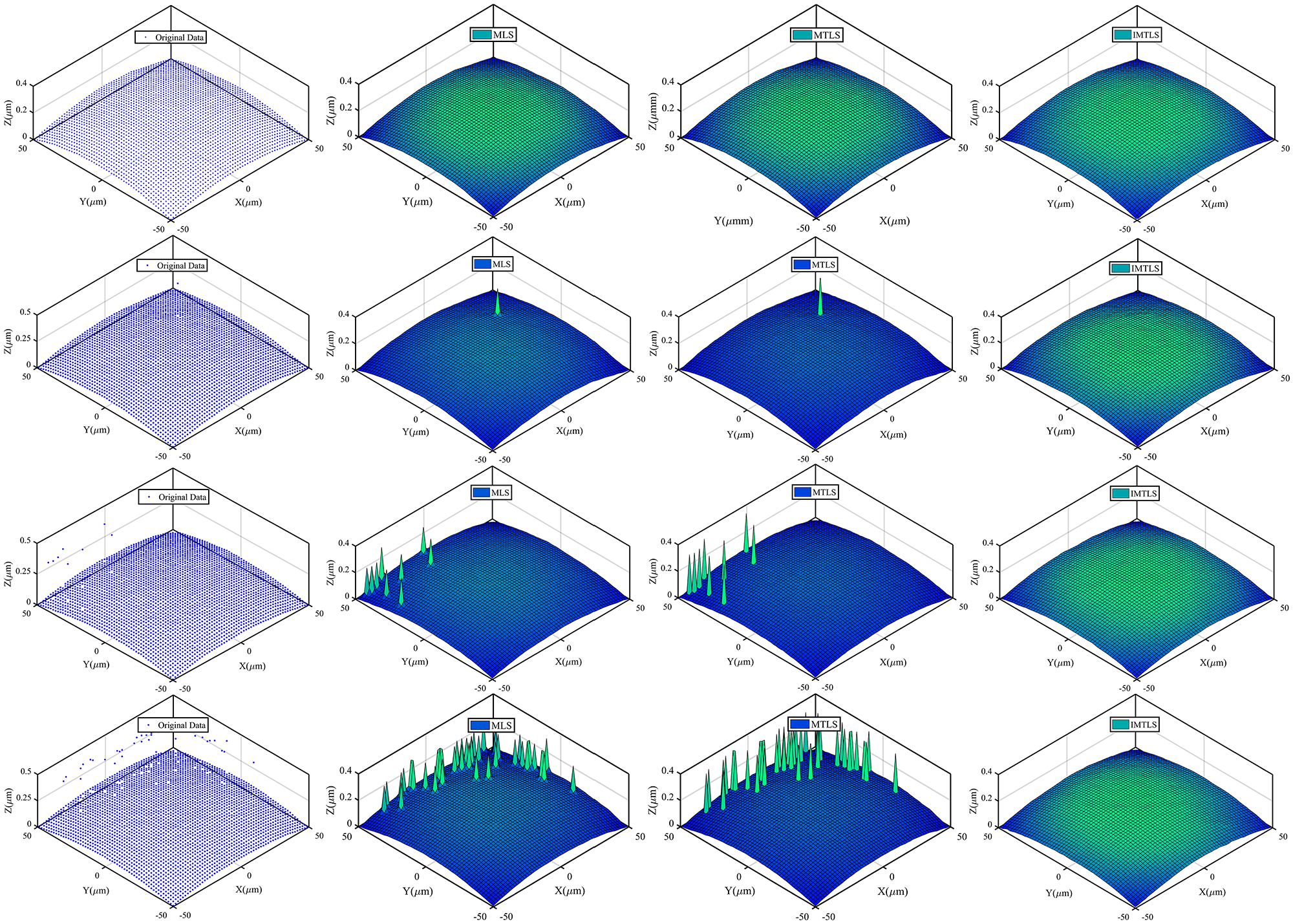
The processing of experimental data.
The regression radii of three methods in Case 2 (mm).
For the correction parameter δ introduced by the IMTLS method, we set different values to observe the change of reconstruction result. As shown in Figure 6(a), when there are outliers in the data, the reconstruction result of the IMTLS method is obviously better than the other two algorithms. And the result will be consistent with that of the MTLS method as δ increases, which shows that when δ increases to a certain value, the node will not be eliminated in the support domain. As shown in Figure 6(b), when there are only random errors, the result of the IMTLS method is still better among the three algorithms. It is clear that δ can be selected in this way for the curve and surface reconstruction.
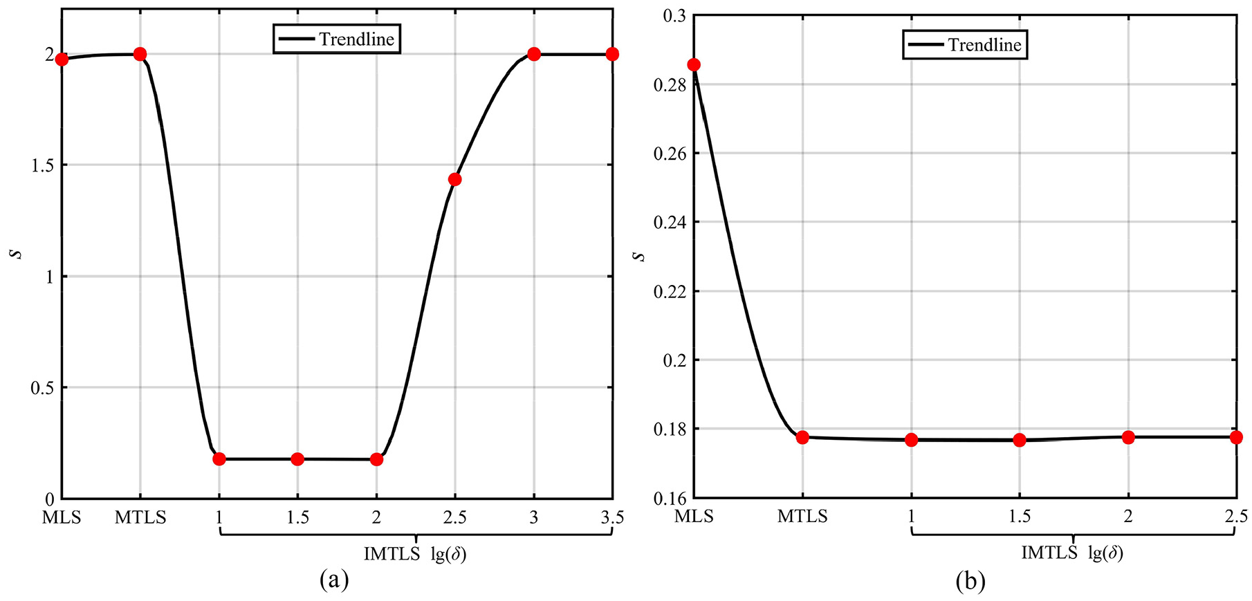
Trendlines of three algorithms in Case 1: (a) the data of the fourth group and (b) the data only containing random errors.
Furthermore, we set different number of nodes that can be eliminated in the support domain, to observe the number of points eliminated in each support domain. The data of the fourth group in Case 2 is taken as an example.
As shown in the Figure 7, the l calculated by the residuals fitted by the LS estimation is relatively large in the support domain with outliers, while in the support domain without outliers, the obtained l is relatively small. Therefore, compared with the support domain without outliers, fewer points are eliminated in the support domain with outliers.
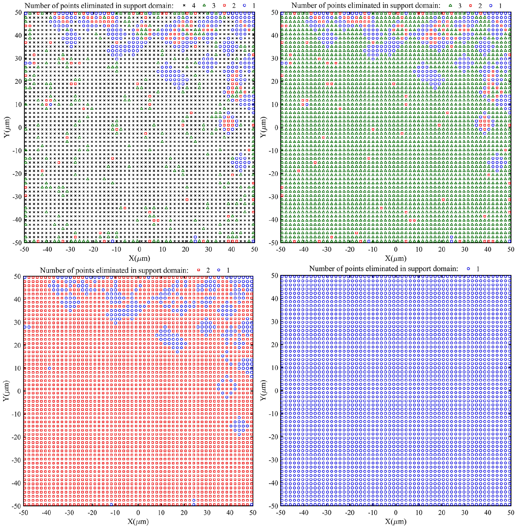
Number of points eliminated in each support domain under different conditions.
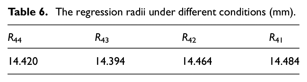
Figure 8 demonstrates the processing result with eliminated nodes, some outliers are not effectively eliminated, because the number of eliminated nodes is not sufficient to eliminate all outliers in some support domains. In addition, the processed data are regressed by simulated annealing to get the regression radii, as shown in Table 6. When the outliers are effectively processed, the corresponding regression radius is significantly closer to the calibrated value. This indicates that the outlier has a great negative influence on the parameter regression and can be processed effectively by setting an appropriate number of elimination nodes.
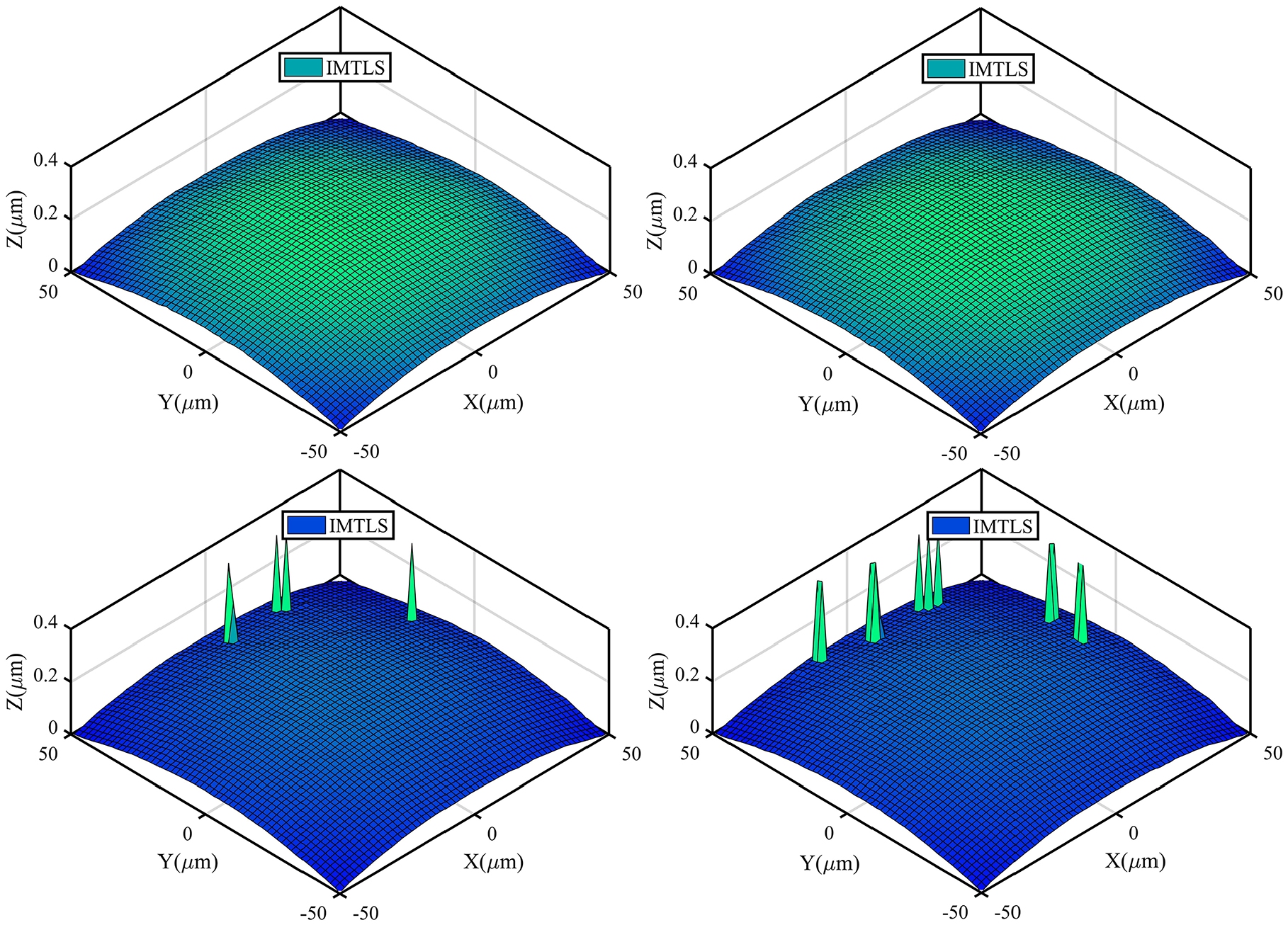
The fitting surface under different conditions.
The regression radii under different conditions (mm).
Through numerical simulation and experimental data verification, the IMTLS method shows better performance. As seen from Case 1, compared with the MLS and MTLS method, the IMTLS method can effectively deal with errors, regardless of whether there are outliers in the data. In addition, the IMTLS method also inherits the good local approximation properties from the MTLS method. We further verify the algorithm by processing measurement data of a standard ball, and the performance of proposed method is evaluated by regression radius. As seen from Case 2, the processed result by the IMTLS algorithm is more proximate to calibrated value.
Conclusion
The MLS and MTLS method show good performance in the fitting of discrete data, such as realizing effective approximation for local geometry feature and obtaining high-order continuous approximation functions with low-order basis functions, etc. However, these two reconstruction methods are not robust, because the outliers in the measurement data will have extremely negative impact on the fitting results. In order to reduce this impact, we proposed an improved MTLS method, in which an improved RANSAC and a correction parameter are introduced into the support domain of the MTLS method to process the abnormal nodes, and then the local fitting coefficients are obtained by the TLS estimation. In this way, the improved MTLS method not only has the advantages of the MTLS method but also can effectively deal with outliers. Practically, we verified the proposed algorithm by dealing with experimental data obtained by CCI. The processing results of three cases show that the performance of the IMTLS method is significantly better than the other two algorithms.
Footnotes
Declaration of conflicting interests
The author(s) declared no potential conflicts of interest with respect to the research, authorship, and/or publication of this article.
Funding
The author(s) disclosed receipt of the following financial support for the research, authorship, and/or publication of this article: This work was supported by the National Natural Science Foundation of China (Grant No. 51605094) and the Fundamental Research Funds for the Central Universities (Grant No. WK2090050042).