
Abstract
Reducing energy consumption in manufacturing is essential for using energy effectively and minimising carbon footprint. In this study, the equation for selecting optimum cutting conditions to minimise energy footprint was extended by considering the fact that as tool wear increases, power and specific energy also increase. This new model enables selecting optimum conditions for energy-smart machining by considering energy footprint, cutting tool utilisation and the volume of material to be removed. This timely research improves the integrity of energy models in machining and their suitability and impact in practical machining conditions.
Introduction
Energy reduction in manufacturing is becoming more critical, due to the increasing impact of industrial emissions as well as the need to minimise costs. Machine tools are one of the resources widely used in manufacturing. Many researchers have investigated the direct energy consumption in machine tools. One of the basic models for direct energy consumption in machining is the model developed by Gutowski et al., 1 as shown in equation (1) presented in Table 1. This model simplified the electrical energy consumed in machining into two main groups, namely, power consumed by the machine tool and power consumed by performing the cutting process.
Direct energy models in machining.
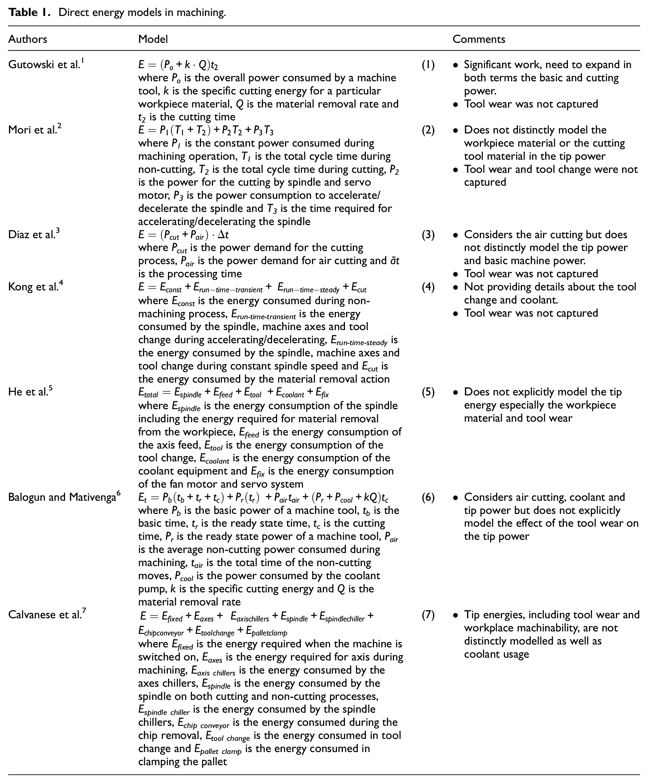
Mori et al. 2 extended the direct energy model to include the ready state power which is the power consumed due to positioning the work to accelerate/decelerate the spindle to a specific speed as seen in equation (2) presented in Table 1. Another model was developed by Diaz et al. 3 The model considered the power consumed in air cutting alongside the actual cutting power (equation (3) in Table 1).
In another step towards smart manufacturing, Kong et al. 4 developed a web-based software and application program interface (API) for evaluating the influence of the toolpath on the environment. The energy model suggested consists of three main stages – non-machining stage, run-time stage (which also consists of two parts), and the cutting stage, as seen in equation (4) presented in Table 1. He et al. 5 presented an energy consumption model based on numerical control (NC) program in machining, as shown in equation (5) presented in Table 1. The model predicts the energy consumption in NC machining and helps to improve the energy consumption in NC program selection. An improved model was suggested by Balogun and Mativenga, 6 which is also shown in equation (6) presented in Table 1. Calvanese et al. 7 proposed an energy model which composes of basic machine power, axes, spindle, chillers and tool change system as seen in equation (7) presented in Table 1.
The equations in Table 1 model the direct energy in machining. In mechanical machining, direct energy demand can be reduced by rapid machining and reducing cycle time. However, such a strategy does not take into account the economic and physics of cutting tool utilisation. A methodology for selecting optimum cutting parameters to minimise energy footprint was developed by Mativenga and Rajemi 8 based on an optimum tool life derived from an energy footprint model that considers both direct energy demand and the energy embodied in the cutting tool and workpiece material. They reported that if the embodied energy of inputs is comprehensively considered, reducing energy in machining can lead to the lower overall cost. This is because there is a synergy between embodied energy and cost. Both parameters address resource effectiveness. This approach was extended by Priarone et al. 9 who added detailed modelling of direct energy consumption for the spindle, axis and lubrication system as well as the energy embodied in the cutting fluid and workpiece material. Table 2 below summarises these previous studies,8,9 modelling the energy footprint E.
Energy footprint models in machining.
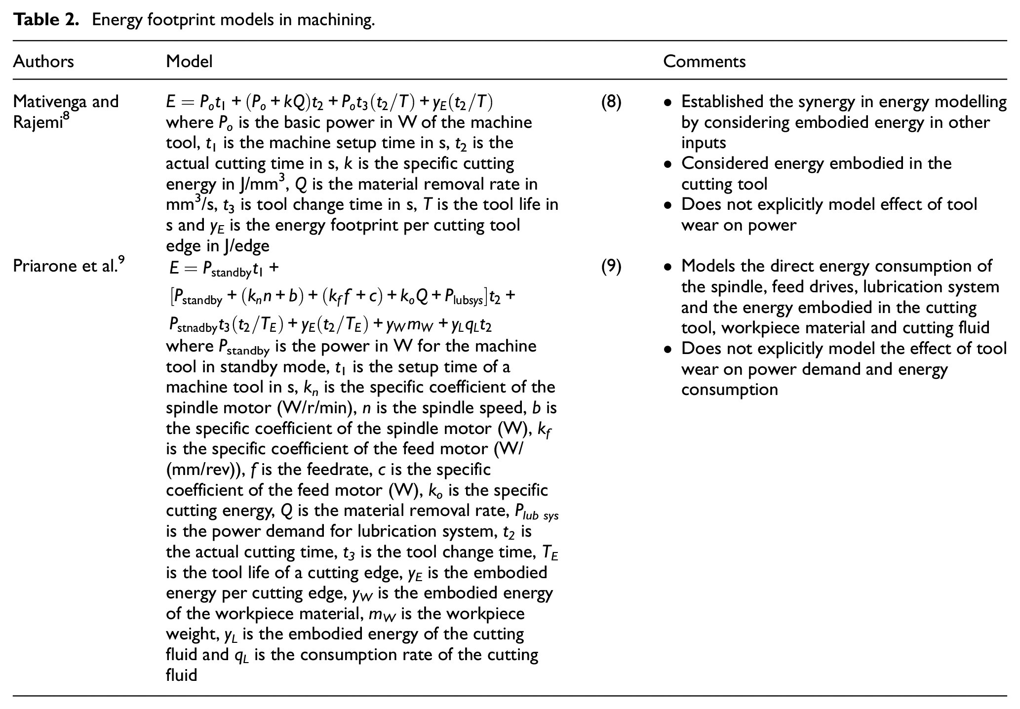
Table 2, equation (8), shows that Mativenga and Rajemi 8 considered energy footprint for tools in their energy footprint model. However, the model did neither capture the effect of tool wear nor was it focused on disaggregated modelling of the direct energy. The energy embodied in the cutting fluid and workpiece material was modelled by Priarone et al., 9 but this had not been extended to explicitly consider that as the tool wears and becomes blunter, the direct and specific energy requirements increase. Based on this premise, the aim of this study was to extend the robustness of the existing mathematical models for selecting cutting conditions, while fully considering the effects of tool wear. The study achieved this through the (i) evaluation and modelling of tool wear demand and its impact on power demand and energy consumption, (ii) extension of the existing energy footprint model to also account for tool wear, and (iii) evaluation of the impact of the proposed model on three selected test case workpieces.
Experimental details and research strategy
Experimental details
To evaluate the impact of tool wear on power demand and energy consumption, cutting tests were undertaken on MHP MT50 CNC Lathe. For measuring the current of the machine tool, a Fluke 434 power logger was used. The current clamp and voltage wires were connected to the machine’s three-phase power supply, as shown in Figure 1.
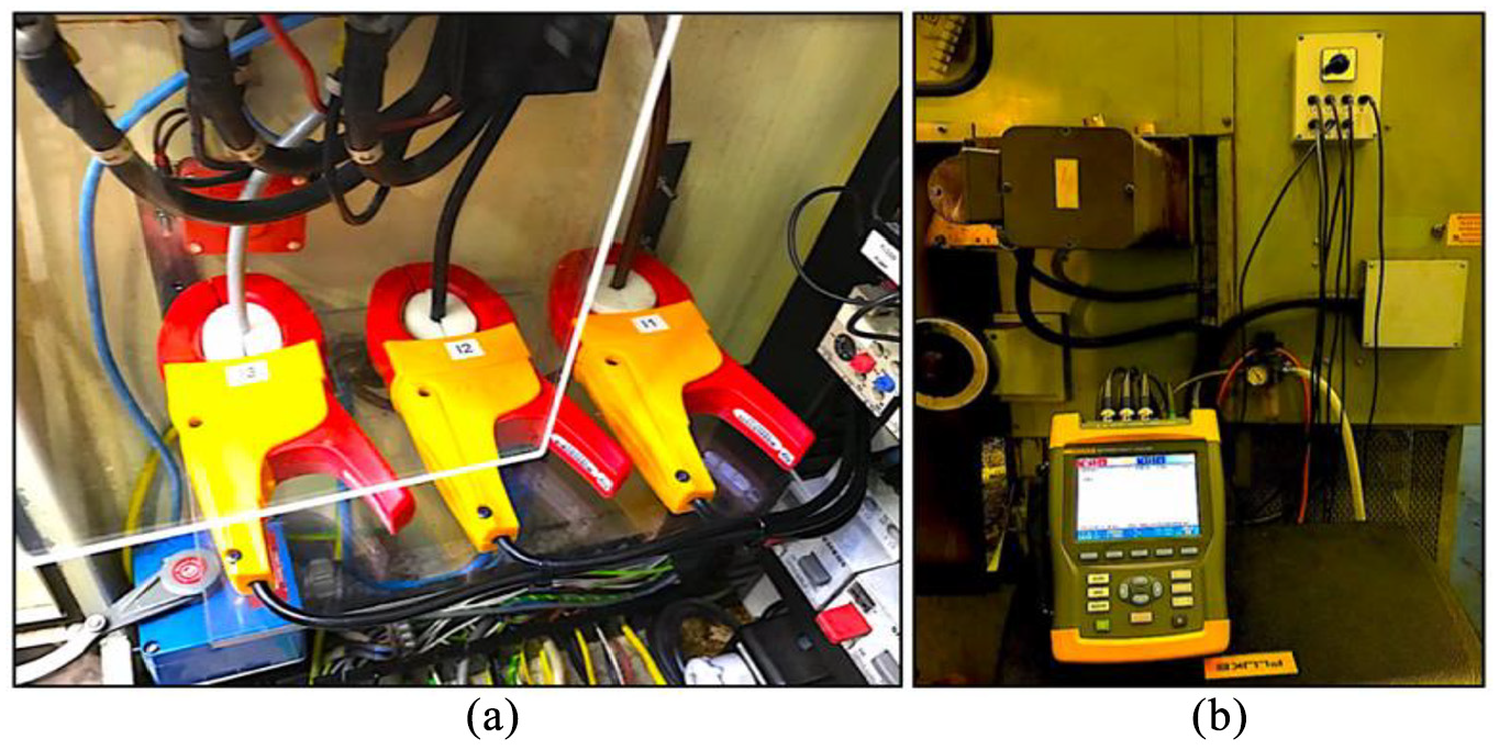
(a) Connection to three-phase in the machine and (b) fluke power analyser connected to a lathe machine.
The machine tool was connected to a three-phase system with a measured line-to-line voltage of 440 V. The total associated power can be modelled by equation (10) 10
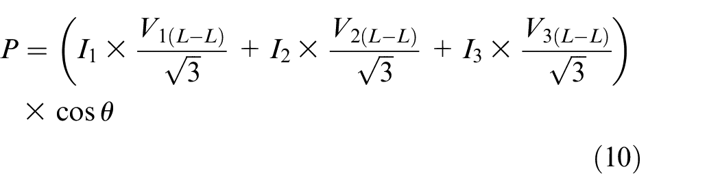
where P is the total power demand in W; the electrical current I1, I2 and I3 are the first, second and third phases, respectively, measured in amperes; V1(L-L), V2(L-L) and V3(L-L) are the line-to-line voltages for the first, second and third phases, respectively, and θ is the phase angle or power factor. The machine had a maximum spindle power of 18.6 kW from 1000 to 3000 r/min, dropping down to 12.3 kW at the maximum spindle speed of 4500 r/min. The maximum current of the machine was 75 A. The measured basic power of the machine was 3346 W.
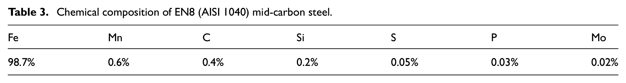
For the evaluation of the tool wear, cutting tests were performed on AISI 1040 carbon steel, as a cylindrical billet. The chemical composition of the workpiece material was measured and is shown in Table 3. The steel was chosen due to its wide use in the industry, especially for shafts, gears, bolts, spindles and other applications that require higher strength than mild steel. The original dimensions of the workpiece bars were 300 mm in length and 130 mm in diameter. Each bar was skimmed to eliminate the effect of any surface inhomogeneity on test results. Each workpiece was then faced down to 298 mm in length with a facing operation of 2 mm and then chamfered to prevent entry damage to the cutting tool edge. Thus, the remaining machined part of the workpiece was 245 mm in length with a 126 mm in diameter. The length of the cut was set to be 200 mm in length.
Chemical composition of EN8 (AISI 1040) mid-carbon steel.
The tool insert was CNMG 120408-WF manufactured by SANDVIK with a material grade of 4315. The tools had a nose radius of 0.8 mm and coated with TiCN + Al2O3 + TiN. The tool holder used was PCLNL 2020k-12. A Quanta 200 scanning electron microscope (SEM) was used for imaging the tools and measuring tool wear.
Research strategy
The first experiment was to evaluate how the power and hence energy demand change with tool use and tool wear. The cutting conditions used were a cutting velocity, Vc, of 415 m/min, a feedrate, f, of 0.15 mm/rev and a depth of cut, ap, of 1 mm. These cutting conditions were chosen based on the tool manufacturer’s recommendation for machining steel material. The cutting time was 25 min, and each test was repeated three times. The current and voltage were measured during cutting. This enabled evaluation of the impact of tool utilisation on cutting power. This was then followed by evaluation of the flank wear (VB) and specific cutting energy k. The specific energy was calculated by plotting the cutting power with the material removal rate for each flank wear progression. The slope of each graph represents the specific energy for each wear progression. For the evaluation of specific energy at defined time intervals over the machining time, 15 cutting tests were done at depth of cut varying from 0.5 to 1.75 mm, while the cutting velocity and feedrate were kept constant as reported before. This enabled to focus on material removal rather than the dominant impact of spindle and feed drives on energy demand.
Results and discussion
Effect of tool wear on cutting power
The effect of the tool utilisation on the cutting power is shown in Figure 2. The overall power of the machine tool rose as the tool utilisation time increased. In this example, the cutting power increased by 50% as the tool was used for 25 min. The specific cutting energy and flank wear were evaluated and measured, respectively, and the results are shown in Table 4.
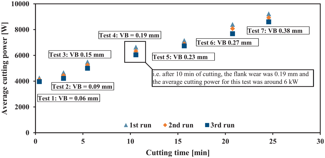
Effect of tool wear on cutting power at a depth of cut of 1 mm, a feedrate of 0.15 mm/rev and a cutting velocity of 415 m/min.
Summary of results of specific cutting energy evaluation.
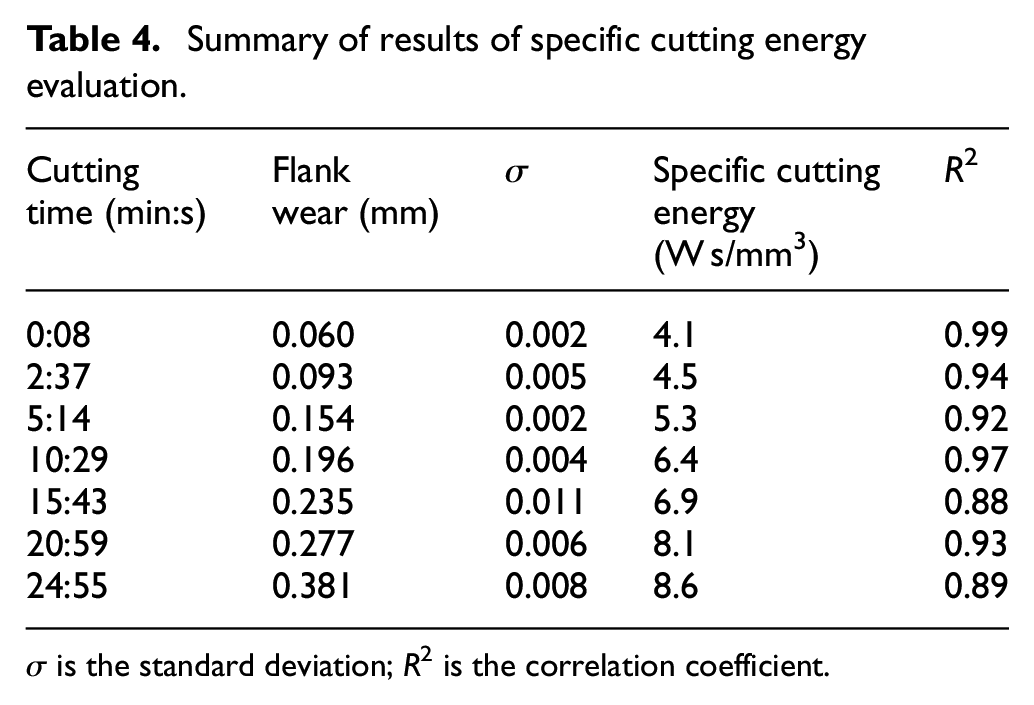
σ is the standard deviation; R2 is the correlation coefficient.
The results of this experiment showed that the specific cutting energy ranged from 4.1 to 8.6 W s/mm3, which is comparable with earlier studies shown in Table 5.11–16 Recent work by Guo et al. 17 was not focused on similar workpiece material class. This increasing body of evidence at tool wear driving increase in specific energy needs to be considering in modelling so that machining optimisation is more realistic and does not assume sharp tools.
Benchmark of specific cutting energy in literature for turning operations.
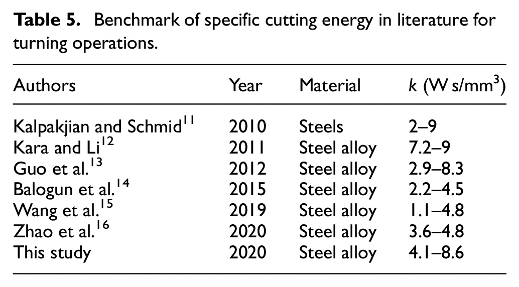
Figure 3 plots the increasing relationship between specific energy and flank wear (VB), and Figure 4 shows how the flank wear (VB) increases with the machining time. A linear regression equation is used to describe the relationship between the flank wear with the cutting time and the specific energy with the flank wear. However, the coefficient of determination (R2) of the linear regression equation is more than 95% in both graphs, and it can be concluded that the linear regression equation can be used to describe the aforementioned relationship. The validity of this trend has to be tested for other workpiece materials and cutting conditions. In this study, up to 0.38 mm of average flank wear was considered in the specific cutting energy model to satisfy the ISO3685 standard for tool life testing with single-point turning tools, which recommends an average flank wear tool life criterion of 0.3 mm. 18
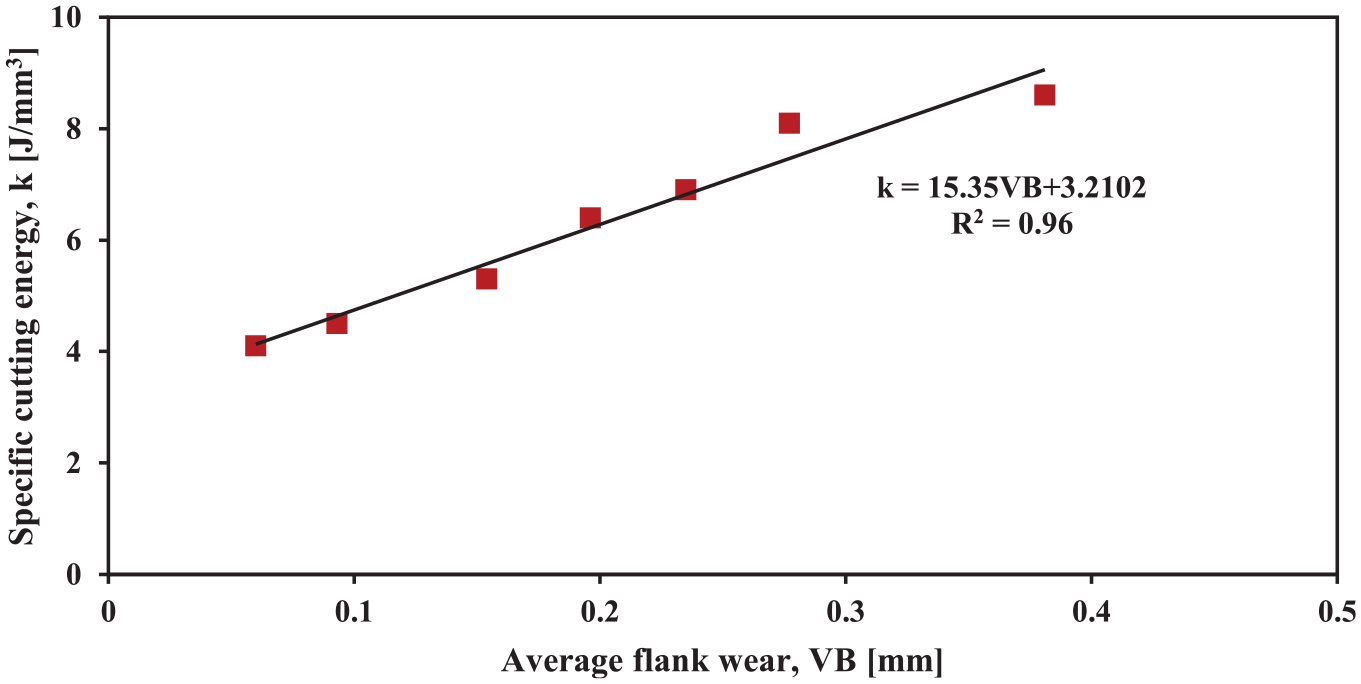
Effect of flank wear on specific cutting energy.
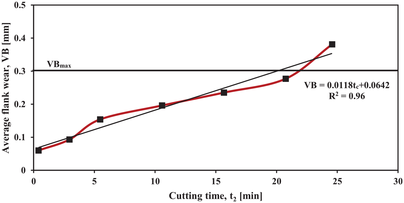
Effect of machining time on flank wear.
From the trends in Figures 3 and 4, equations (11) and (12) are obtained and these are then combined to yield equation (13)


where k is the specific cutting edge in J/mm3, VB is the flank wear in mm and t2 is the cutting time in seconds. The parameters, 0.003 and 4.20, can be taken as constants C1 and C2 with units of specific power and energy, respectively. However, this part of the model is valid when using the same workpiece material and the same tool insert. The relationship between the specific energy versus flank wear and flank wear versus cutting time is based on the cutting tool and the workpiece material used. Thus, this relationship needs to be set according to the workpiece/tool used.
An improved energy footprint model considering tool wear
From the experiment, the relationship between the specific cutting energy and cutting time was captured in equation (13). Thus, the general formula for estimating specific cutting energy with machining time in equation (13) (also considering tool wear) can be written as equation (14)

where k is the specific cutting energy, t2 is the cutting time, C1 is the specific power in W/mm3 and C2 is the specific cutting energy of a new tool insert in J/mm3.
Consequently, this new relationship can be applied to the energy footprint model for machining, equation (8) in Table 2 to take into consideration the change in specific cutting energy due to tool wear during cutting. In order to achieve this, the second term (tip energy) of the energy footprint model (Po + kQ)t2, which was developed by Gutowski et al. 1 and it represents the energy consumed during actual cutting in turning, E2, can be written as equation (15)

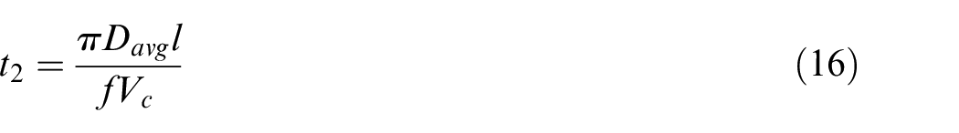
where the cutting time t2 is the cutting time modelled by equation (16)
The material removal rate Q can be expressed as follows
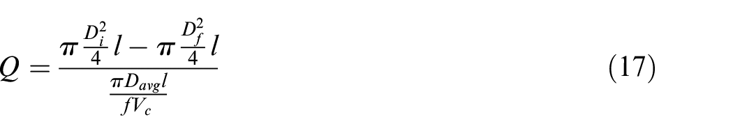
By substituting equations (16) and (17) into equation (8) in Table 2, the total energy footprint equation E can be written as equation (18)
By substituting the tool life using Taylor’s extended tool life equation 19 into equation (18), for a single pass of turning and hence constant depth of cut, equation (19) is obtained
Equation (19) can be reorganised as equation (20)
The fundamental rationale behind optimisation is to obtain an optimum tool life that satisfies the minimum energy footprint criteria. This tool life can then be used in the tool life equation to obtain an optimum cutting velocity for minimum energy criteria. The optimum tool life for minimum energy criteria is obtained by differentiating the energy footprint E with respect to the cutting velocity Vc and equating it to zero, and this yields
After simplifying, the optimum tool life equation for minimum energy criterion taking into account direct energy, the impact of tool wear and the energy embodied in the cutting tool can be written as equation (22)
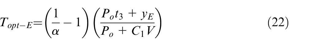
where Topt-E is the optimum tool life for minimum energy criteria. The cutting velocity exponent (1/α) is derived from tool wear tests and is influenced by the machinability of the workpiece material and the wear rate of the cutting tool used. Po is measured from machine energy consumption and yE is calculated from the energy footprint in the cutting tool. The energy footprint of a cutting tool can be calculated by adding the energy embodied in tool material production, considering tool insert weight, to the energy consumed in coating and tool manufacture (the sintering process, in this case). Dahmus and Gutowski 20 provided the energy embodied in cutting tool. Po can be disaggregated into, for example, power for lubricant system, spindle system, and feed drives, as modelled by Priarone et al. 9 For utility and simplicity in this article, the basic power is used.
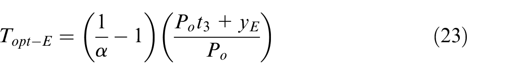
From equation (22), the tool life velocity exponent (the rate at which tool life reduces with increasing cutting speed), the basic power of the machine, the non-productive total time for tool change time and energy footprint for cutting tools are the key elements influencing the selection of optimum tool life for achieving minimum energy consumption. Comparing equation (22) with the original tool life equation in work done by Mativenga and Rajemi, 8 equation (23), the new addition to the model for optimum tool life is the machined volume
Each tool has a limited volume that it can remove. It is suggested that in this model, the volume can be set by considering the minimum and maximum tool life. For example, tool life of 10 and 100 min for minimum and maximum is used. The lower limit avoids uneconomic use of cutting tools, while the upper limit avoids tool thermal expansion. This can be calculated from the process window for a given cutting tool and workpiece combination. The new improved model can be applied based on the methodology of selection of cutting condition as extensively covered by Mativenga and Rajemi 8 and Priarone et al. 9
The inferred understanding from equation (22) is that if cutting tools of high embodied energy are used, then a more conservative cutting velocity is required in order to extract more value from the tooling. If a high volume of material is to be removed by the same tool, then the cutting process is done at a higher velocity in order to reduce the cycle time and direct energy (which increases with tool wear).
Equation (22) is an elegant solution because it points out that by knowing the total volume to be removed, it is possible to address the impact of tool wear on energy optimisation in machining.
Optimisation example
From the optimum tool life model for minimum energy criterion shown in equation (22), it can be observed that the optimum tool life for minimum energy is inversely proportional to the volume to be removed. To illustrate the effect of considering tool wear on the developed model, three components were selected to be machined as can be seen in Figure 5. The three components are made of mid-carbon steel (AISI 1040) and all require the same turning operation, that is, forward turning operation. The cutting insert was CNMG 120408-WF manufactured by SANDVIK for finishing cut. A combination of cutting parameters is done for the recommended cutting conditions by the tool manufacturer, the mid-range cutting conditions and the optimised cutting conditions using the extended model in this research. Then, the total energy is compared to other models. The selection of optimum cutting conditions to minimise energy footprint follows the procedure reported before, by Mativenga and Rajemi, 8 and this procedure is summarised in Figure 6.
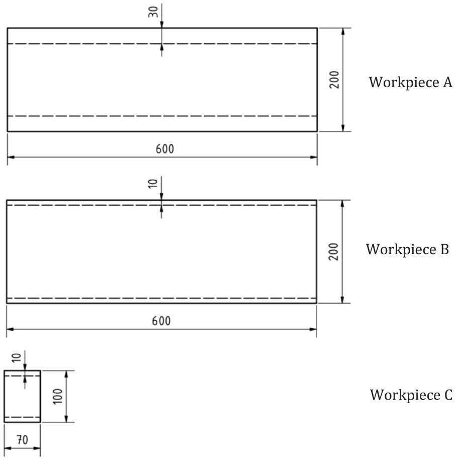
The three workpieces used in this example (all dimensions in mm). The dashed area shows the total depth of cut.
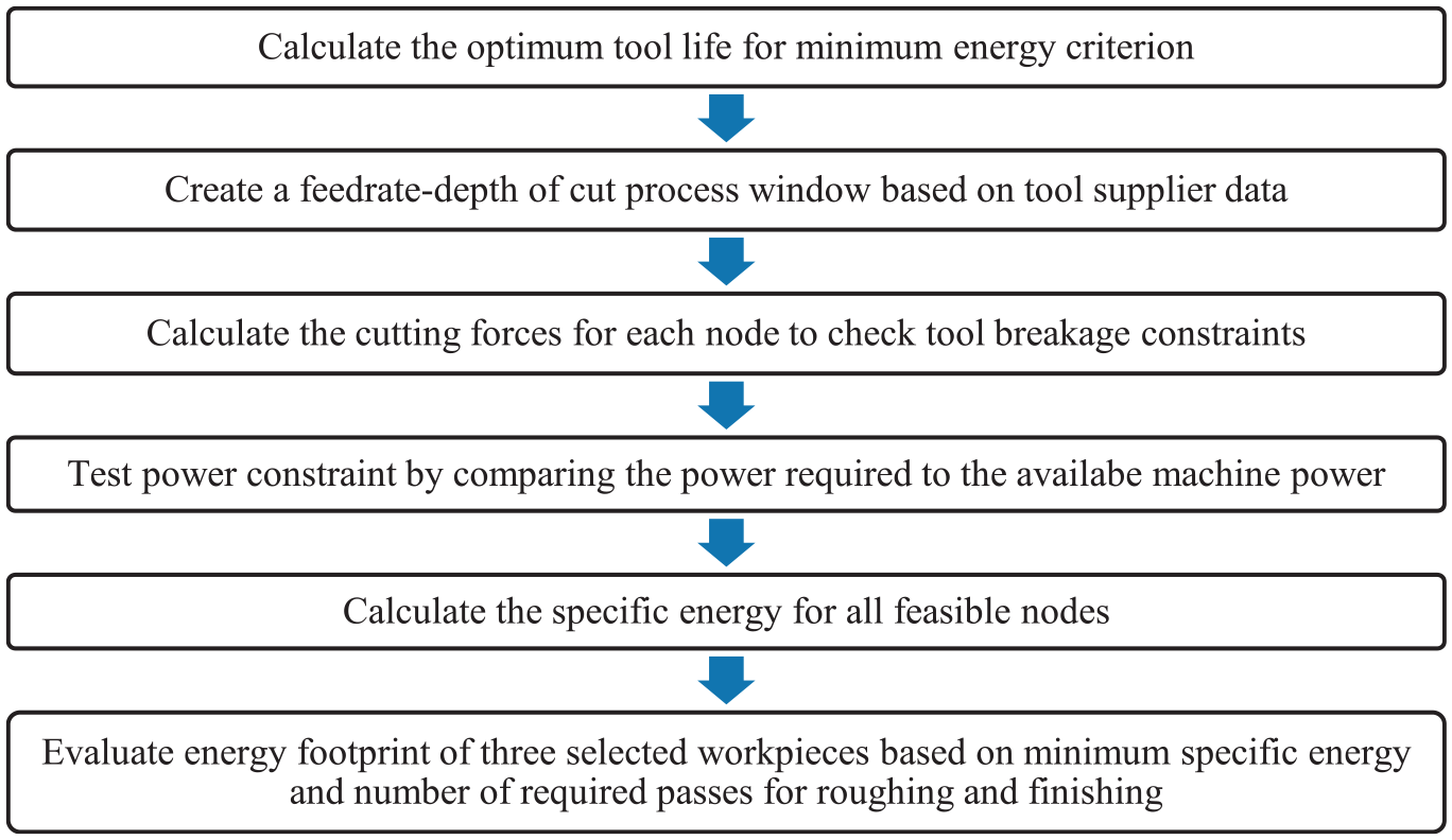
Optimisation procedure.
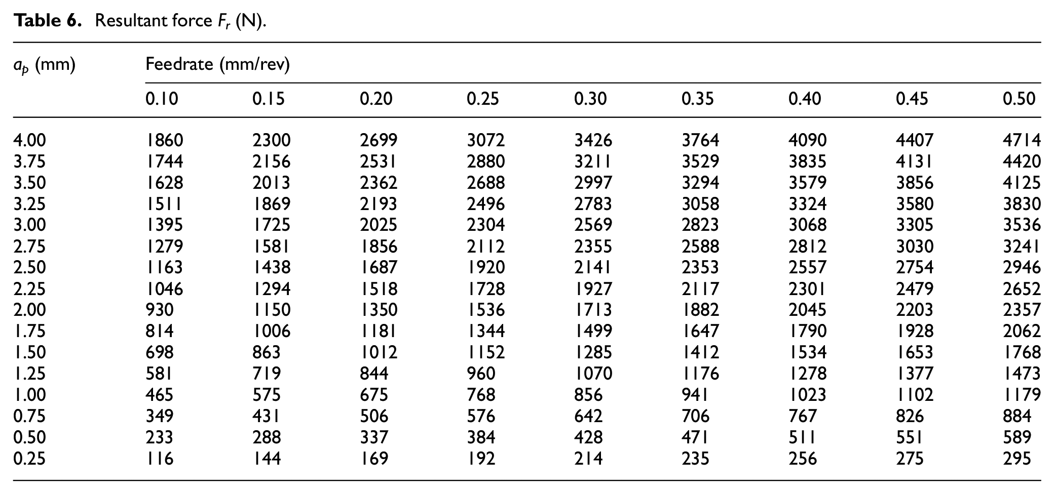
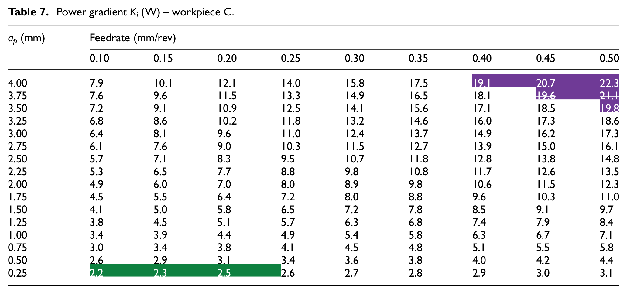
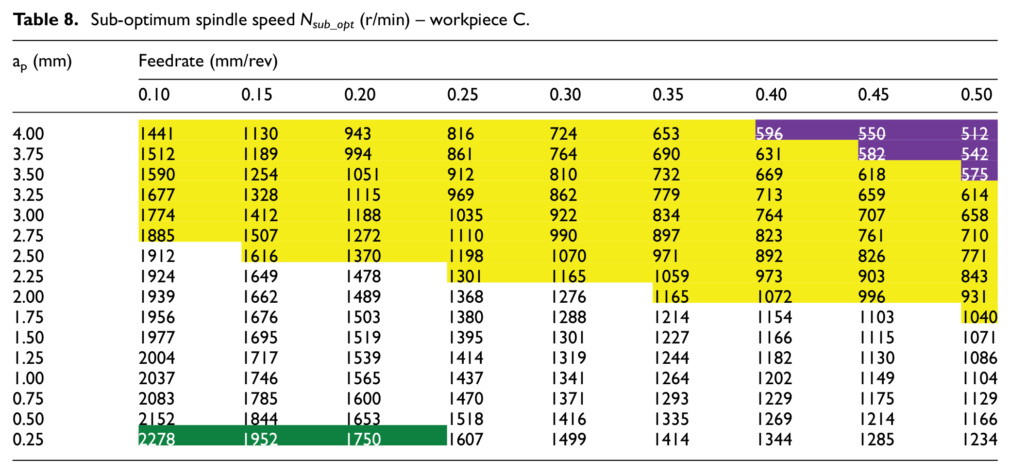
Tool breakage constraint was checked by evaluating the cutting forces. Table 6 shows the resultant force Fr for the tool insert used. The maximum force to break the insert 8 was 5500 N, and hence it is clear from the table that all the nodes did not violate the force constraint. The power constraint was evaluated using two reference power gradients k1 = 18,600/1000 = 18.6 (maximum spindle power with load at 1000 r/min) and k2 = 11,400/4600 = 2.5 (maximum available power for spindle with load at 4600 r/min) compared to the power for the minimum energy footprint ki as shown in Figure 7. Any gradient above 18.6 is not feasible and highlighted in purple, as seen in Table 7. Any gradient below 2.5 might be still feasible if the calculated spindle speed was less than 4600 r/min, this was highlighted in green. Then, the sub-optimum spindle speed was found by comparing the optimum spindle speed with the original spindle speed as explained in Figure 7. The modified spindle speed was highlighted in yellow, as shown in Table 8.
Resultant force Fr (N).
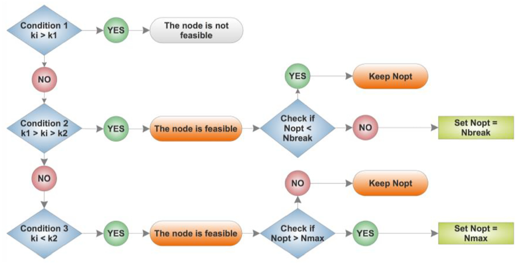
Flowchart of the procedure for testing the machining conditions that can be performed within the available machine power.
Power gradient Ki (W) – workpiece C.
Sub-optimum spindle speed Nsub_opt (r/min) – workpiece C.
The new cutting velocity Vc_New based on the modified Nsub_opt is shown in Table 9. The cutting velocity which has values above or below the recommended range (i.e. minimum Vc = 335 m/min and maximum Vc = 555 m/min) based on tool supplier recommendation was highlighted in red whereas these velocities are not applicable in machining processes.
New cutting velocity Vc_New (m/min) – workpiece C.
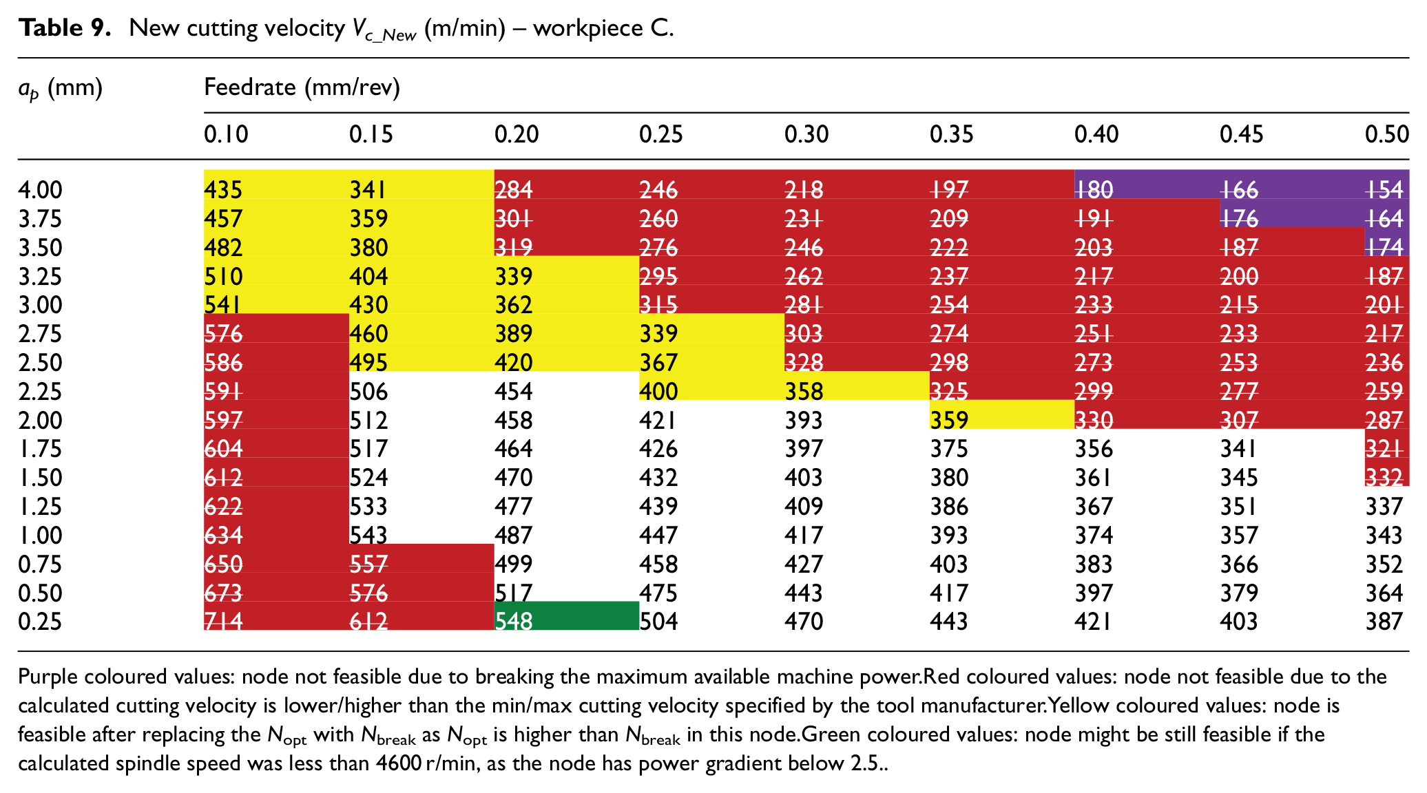
Purple coloured values: node not feasible due to breaking the maximum available machine power.Red coloured values: node not feasible due to the calculated cutting velocity is lower/higher than the min/max cutting velocity specified by the tool manufacturer.Yellow coloured values: node is feasible after replacing the Nopt with Nbreak as Nopt is higher than Nbreak in this node.Green coloured values: node might be still feasible if the calculated spindle speed was less than 4600 r/min, as the node has power gradient below 2.5.
After considering the tool breakage constraint, the available power constraint and the cutting velocity constraint, it can be observed that the process window is narrowed down after applying each constraint which helps in selecting the optimum cutting conditions. The minimum specific energy per unit volume required for turning workpiece A, workpiece B and workpiece C were used to select the optimum set of cutting conditions. The effect of feedrate and depth of cut on specific energy for workpiece A, workpiece B and workpiece C is shown in Tables 10, 11 and 12, respectively. From the tables, it can be seen how the feedrate and the depth of cut affect the specific energy, as machining with higher feedrate and depth of cut can result in reducing the specific energy. In the case of workpiece A, the minimum energy per volume removed was 5.70 W s/mm3. The cutting conditions of this node are as follows: a cutting velocity of 397 m/min, a feedrate of 0.15 mm/rev and a depth of cut of 3.75 mm, as shown in Table 10. As the extended model in this research considers the volume to be removed and workpieces A and B have much more material to be removed compared to workpiece C, workpieces A and B have reached the lower limit of the optimum tool life for minimum energy which is 10 min. This limit was set in order to make the machining process more efficient in terms of non-productive time due to frequent tool changes. So as can be seen from Table 11, the minimum energy per volume removed for workpiece B was similar to workpiece A which was 5.70 W s/mm3. This can be achieved by a cutting velocity of 397 m/min, a feedrate of 0.15 mm/rev and a depth of cut of 3.75 mm. However, workpiece B has more feasible nodes than the workpieces A and B due to less volume of the material to be removed compared to the other workpieces. From Table 12, the minimum energy per volume removed for workpiece C was 10.15 W s/mm3 using a cutting velocity of 341 m/min, a feedrate of 0.15 mm/rev and a depth of cut of 4.00 mm. The study illustrates the changes in machining small components with a large machine tool. The economics of energy utilisation is not favourable when small components are machined down on machine tool that has large basic power.
Specific energy (W s/mm3) for workpiece A.

Shaded areas without strike-through violate process constraints and can be made feasible through a sub-optimum solution.
Shaded and strike-through areas violate process constraints and are not feasible.
Specific energy (W s/mm3) for workpiece B.
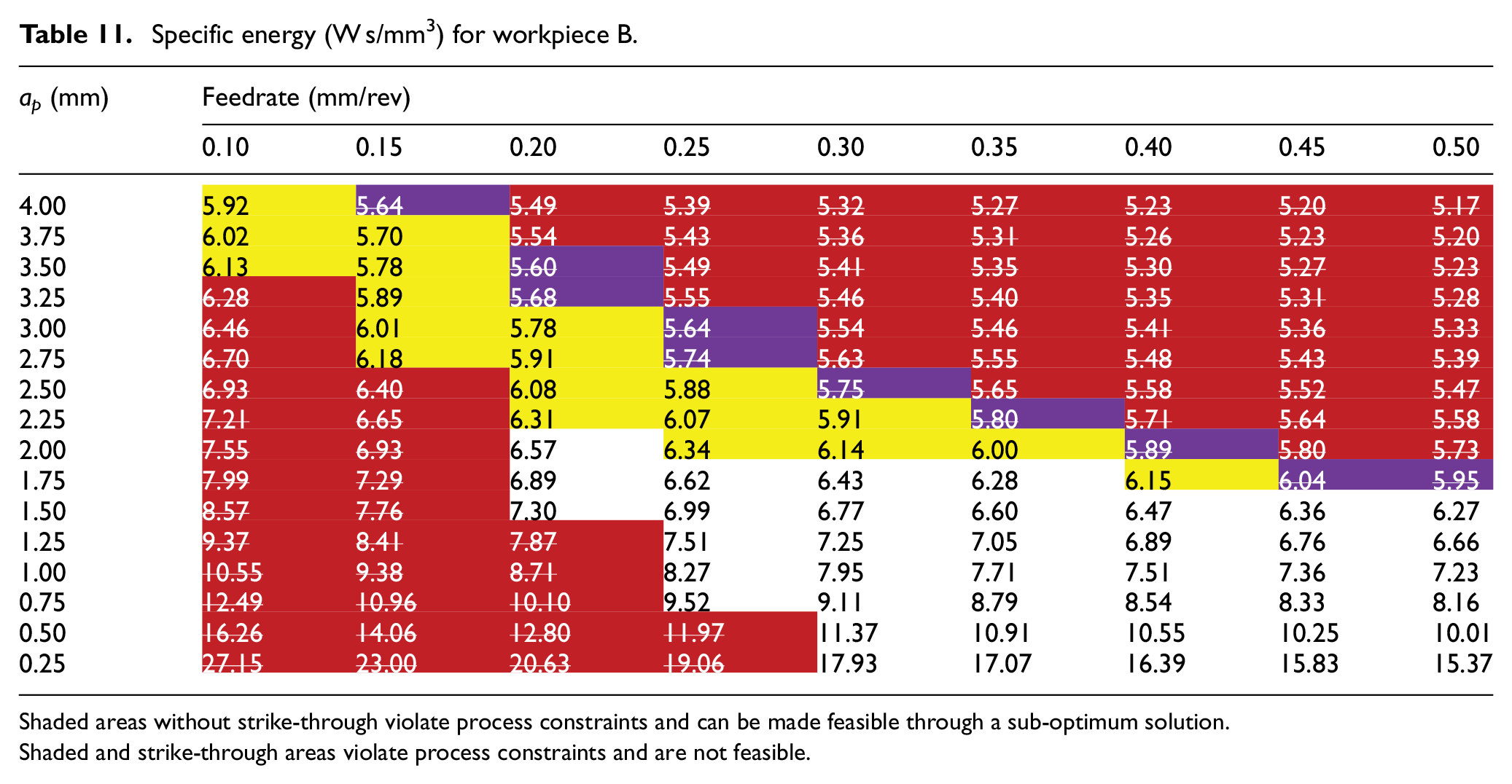
Shaded areas without strike-through violate process constraints and can be made feasible through a sub-optimum solution.
Shaded and strike-through areas violate process constraints and are not feasible.
Specific energy (W s/mm3) for workpiece C.
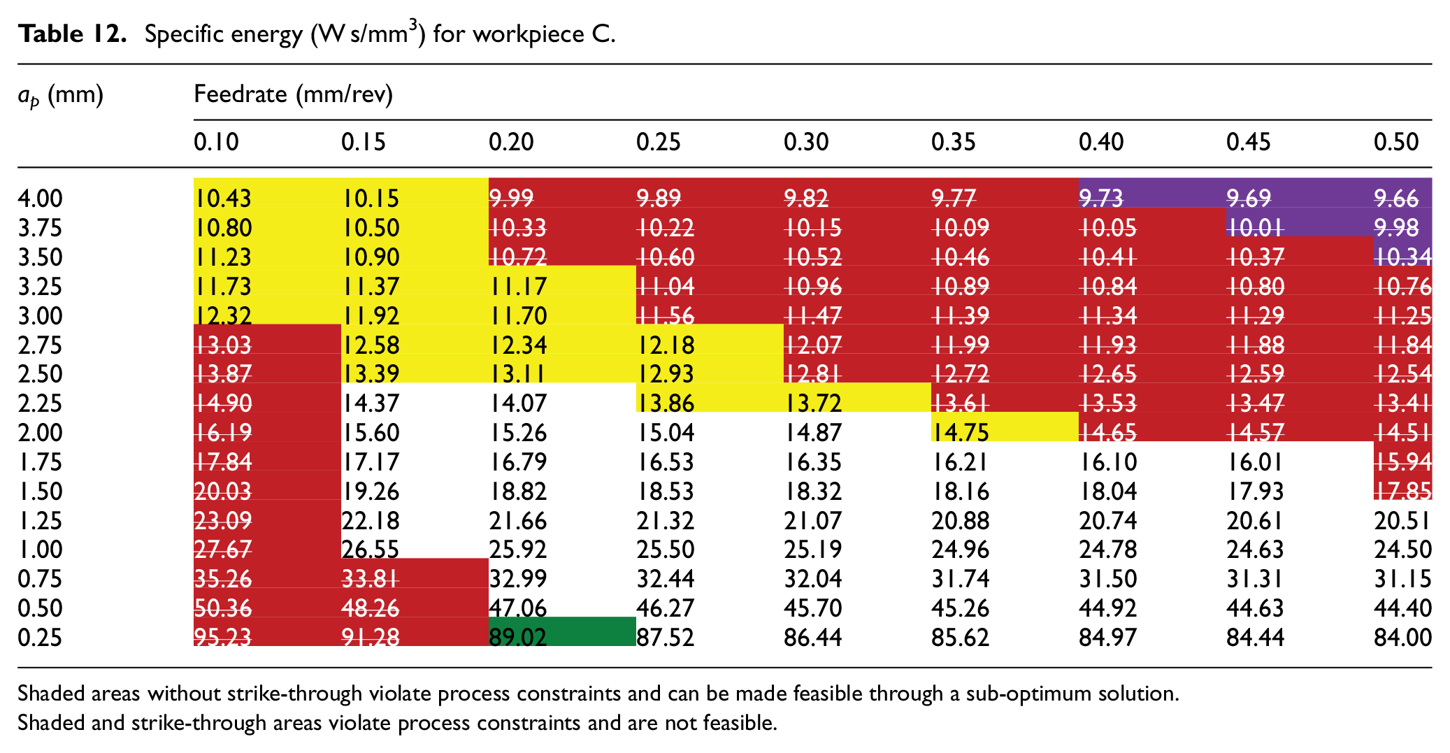
Shaded areas without strike-through violate process constraints and can be made feasible through a sub-optimum solution.
Shaded and strike-through areas violate process constraints and are not feasible.
The total energy from the optimum cutting conditions was compared to the tool supplier recommended cutting variables and process window mid-range parameters. The results are shown in Table 13. For the larger workpiece considered, the energy footprint was reduced by 28% when using the optimum conditions from the improved model and comparing this to the tool supplier recommended conditions. The results also show that roughing using process window mid-range conditions is a crude estimate for reducing the energy requirement in machining.
Cutting conditions for the optimum solution compared to the recommended and mid-range parameters.
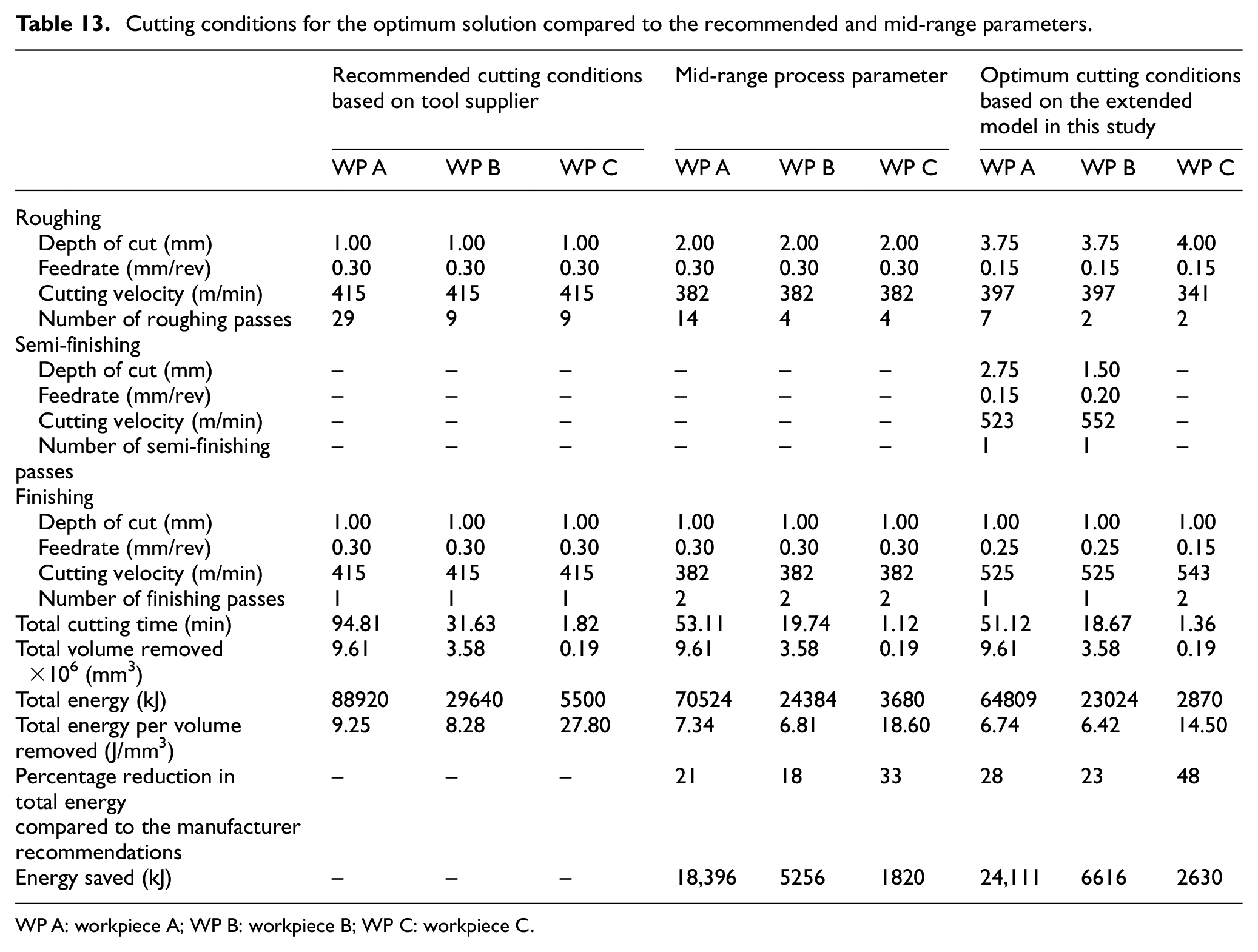
WP A: workpiece A; WP B: workpiece B; WP C: workpiece C.
Conclusion
The main findings from this study can be summarised as follows:
There is a need to increase the integrity of models used for the selection of cutting conditions. If the selection is based on direct energy the conclusion is that rapid machining should be used. However, this does not optimise the usage of cutting tools and other inputs that have embodied energy; it can also compromise component quality. The use of energy footprint models and realistic modelling of the impact of tool wear improves the integrity of energy models.
In this study, tool utilisation and hence tool wear were found to increase the cutting power by 40% over a cutting time of 25 min and a flank wear land of 0.15 mm. This suggests that the impact of tool wear on direct energy demand is significant and should not be neglected in energy modelling. It can be inferred that this impact can be even more significant if the tool is used to 0.2 or 0.3 mm flank wear.
By modelling how the specific cutting energy changes with tool wear and hence cutting time, the energy footprint model for turning was improved. A new equation for optimum tool life for minimum energy was developed and this captures the volume of the workpiece. The core relevance of the currently proposed approach is that the user can simply calculate the volume to be removed and hence account for the impact of tool sharpness on energy demand. This is a simple and convenient way for modelling energy demand in machining.
The longer the cutting time and the higher the volume of material to be removed by a single tool, the more significant it is to consider the impact of tool wear on specific energy required.
Footnotes
Declaration of conflicting interests
The author(s) declared no potential conflicts of interest with respect to the research, authorship, and/or publication of this article.
Funding
The author(s) received no financial support for the research, authorship, and/or publication of this article.