Sage Journals: Discover world-class research

Abstract

Recently, the emerging rail grinding method using abrasive belt has been proposed to efficiently achieve the required geometric profile and the surface quality of the railhead. Although the abrasive features indeed have a great influence on this rail grinding process, the surface topography of abrasive belt regarding grits at the microscopic scale is neglected. In this article, a microscopic contact pressure model was developed to reveal the contact behavior of every active grit based on the digital representation of the surface topography of abrasive belt. Then a numerical model of material removal quantity was also established based on the consideration of the characteristics of abrasive grits and their interactions. Finally, the series of finite element simulations and grinding tests were successively implemented. The normal load and the surface topography of abrasive belt significantly affected the microscopic contact behavior of grits, thus confirming the proposed theoretical models of microscopic contact pressure and material removal quantity.

Keywords

Rail grinding abrasive belt contact pressure material removal

Introduction

Rail grinding has been widely recognized as an essential and routine rail maintenance technique since rails inevitably suffer from various defects, such as corrugation, crack, spalling, squat and even fracture.^1,2 Through the periodically preventive or temporarily corrective implementation, rail grinding can effectively remove the flaws mentioned above, preserve rail profiles, reduce train running noise and enhance passengers’ comfort.^3–5

The rail grinding technologies have always been extensively explored. Various grinding technologies, including the face grinding with abrasive wheel,^6–11 the peripheral grinding with abrasive wheel,^12,13 the milling with combined cutter blades¹⁴ and the high-speed grinding with unpowered abrasive wheel,¹⁵ have been applied in different railway circumstances. Furthermore, the new rail grinding method using abrasive belt¹⁶ has also been proposed and has showed the convincing merits, including the higher material removal rate and the better surface quality.

The abrasive belt, as the most typical coated tool with lots of abrasive grits on its working surface, has developed rapidly over the past few decades. Due to its high flexibility and compliance,^17,18 belt grinding naturally has the mixed effect of grinding and polishing. Hence, it has become an effective machining process in industries, including aerospace, ship, nuclear power and automobile, through kinds of handheld devices, robotics^19–22 and computer numerical control (CNC).^23,24 The abrasive belt grinding process also has those advantages in rail maintenance, as demonstrated in Datong–Qinhuangdao heavy haul railway in China, which was ground by an innovative rail grinding device using abrasive belt, as shown in Figure 1.

Figure 1.

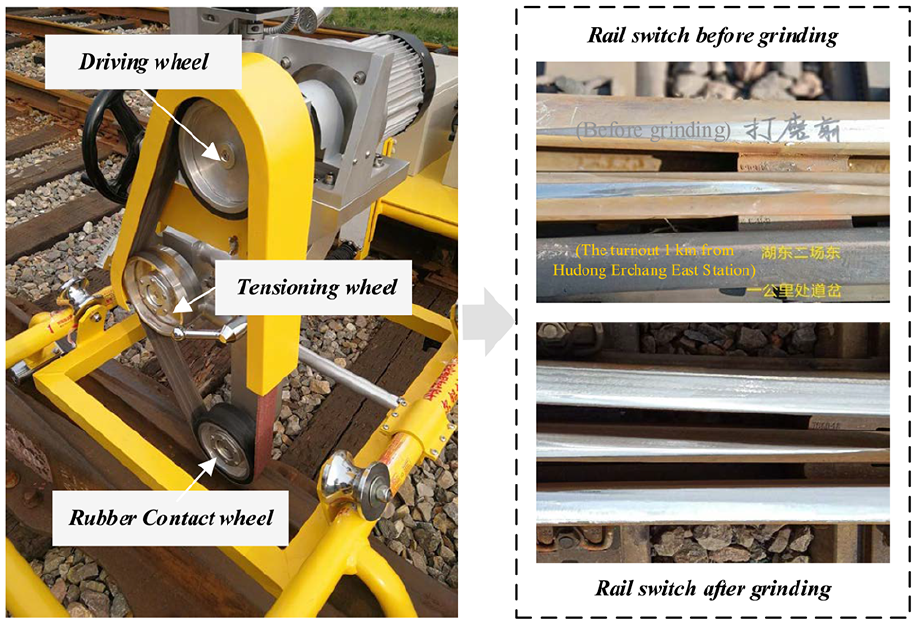
Actual effect of rail grinding using abrasive belt.

The rail grinding process utilizing abrasive belt involves intricate multi-body interactions between the rubber wheel, the abrasive belt and the rail surface. Sun et al.²⁵ investigated the pressure distribution at the interface between a serrated rubber wheel and the workpiece. Experimental and simulation results provided a good understanding of this contact behavior mode. Afterward, Fan et al.²⁶ and Wang et al.²⁷ developed numerical models of macro contact behaviors and material removal mechanism, respectively, for the rubber wheel with a concave peripheral surface.

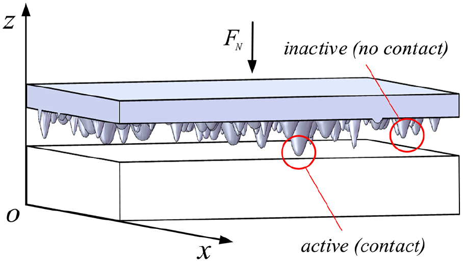
However, the surface topography regarding grits on abrasive belt at the microscopic scale is neglected. In fact, the abrasive feature indeed has a great influence on the material removal, temperature field, abrasive abrasion and final surface texture.^28–30 The real contact zone is not the theoretical ellipse any more, but the set of all contact spots (called microcontacts³¹) corresponding to the pressure distribution area of all active grits, as shown in Figure 2. The micro-grain scratching study adopted a novel approach, single diamond grain grinding at the nanoscale depth at m/s, which was three- to six-order magnitude higher than nanoscratching at mm/s and μm/s, to investigate the fundamental mechanisms of abrasive machining.³² The grinding speed used in the above approach was in good agreement with pragmatic abrasive machining, displaying the significant breakthrough compared to conventional nanoscratching.³³ Under the guidance of the novel approach, mechanical chemical grinding and new diamond wheels were developed.^34,35

Figure 2.

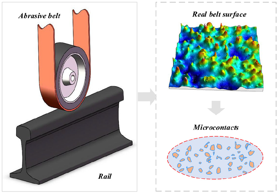
Schematic diagram of microcontacts for rail grinding using abrasive belt.

Therefore, this study aims to investigate the microscopic contact behavior of rail grinding using abrasive belt and reveal the contact status of each grit. A new numerical model of material removal quantity was established based on the characteristics of abrasive grits and their interactions. In addition, the finite element (FE) simulations and grinding tests were implemented to verify these models.

Microscopic contact pressure model

The surface topography of abrasive belt is composed of randomly distributed abrasive grits with different shapes, so the grinding mechanism is complicated. To understand the microscopic contact behavior, the surface topography of abrasive belt should be described as real as possible to lay a foundation for the subsequent contact pressure modeling and FE analysis.

Digital representation of the surface topography of abrasive belt

The original surface topography of abrasive belt was scanned by a 3D non-contact Nanovea PS50 profilometer composed of a white light chromatic sensor P1-OP3500, a platform and a signal processor,³⁶ as shown in Figure 3. Its basic parameters are provided as follows: maximum vertical measurement range (3 mm), depth resolution (25 nm), depth accuracy (200 nm), maximum planer resolution (2.6 μm), maximum measurable gradient (87°) and minimum horizon sample interval (0.1 μm).

Figure 3.

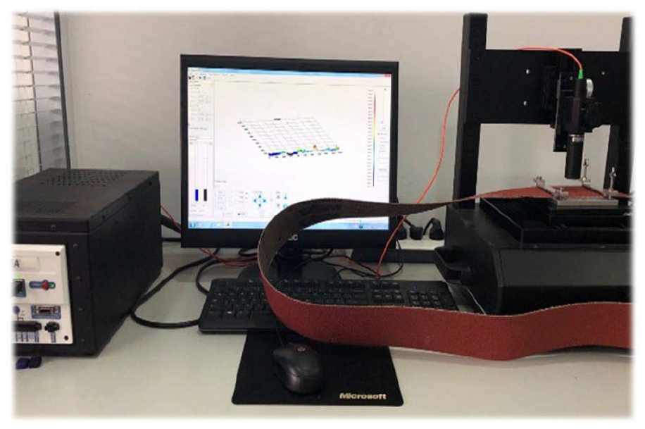
Non-contact Nanovea PS50 profilometer.

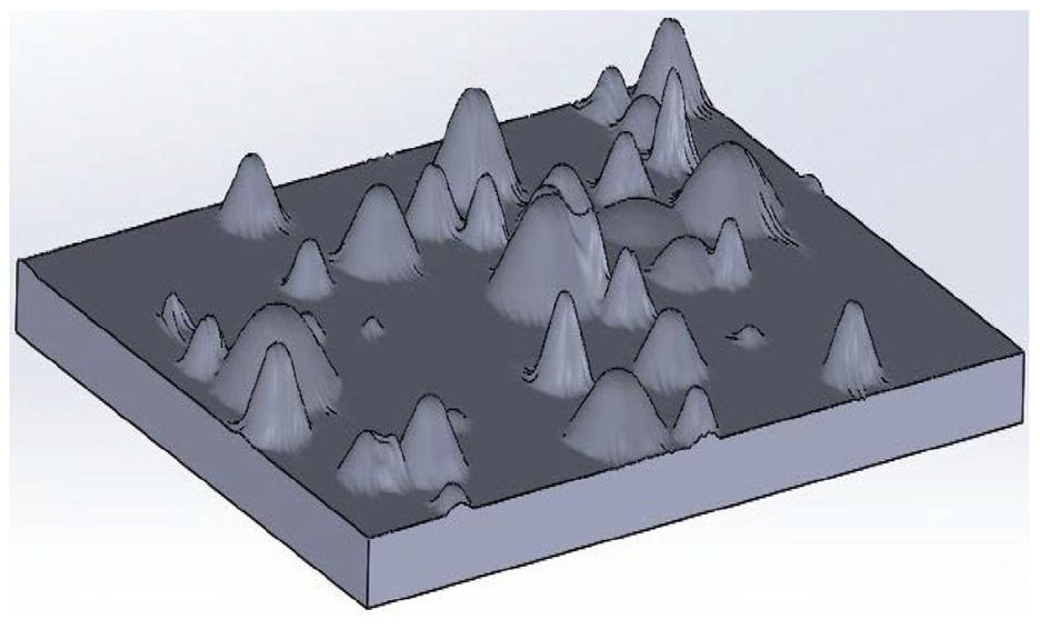
In this study, the representative surface region of the abrasive belt restricted by 10 × 10 mm² was chosen as the investigation object. The horizon sample interval was set to 0.5 μm. Taking VSM-40 ceramic abrasive belt as an example, 4 × 10⁸ measuring points were totally obtained to draw the outline of the belt surface topography (Figure 4(a)). The geometry of single abrasive grit was described as a cone with a spherical end tip. The position, height and attack angle of each abrasive grit could be extracted as the three indices to form the abrasive belt surface (Figure 4(b)). Then, the 3D entity model of the belt shown in Figure 4(c) was used in the FE simulation.

Figure 4.

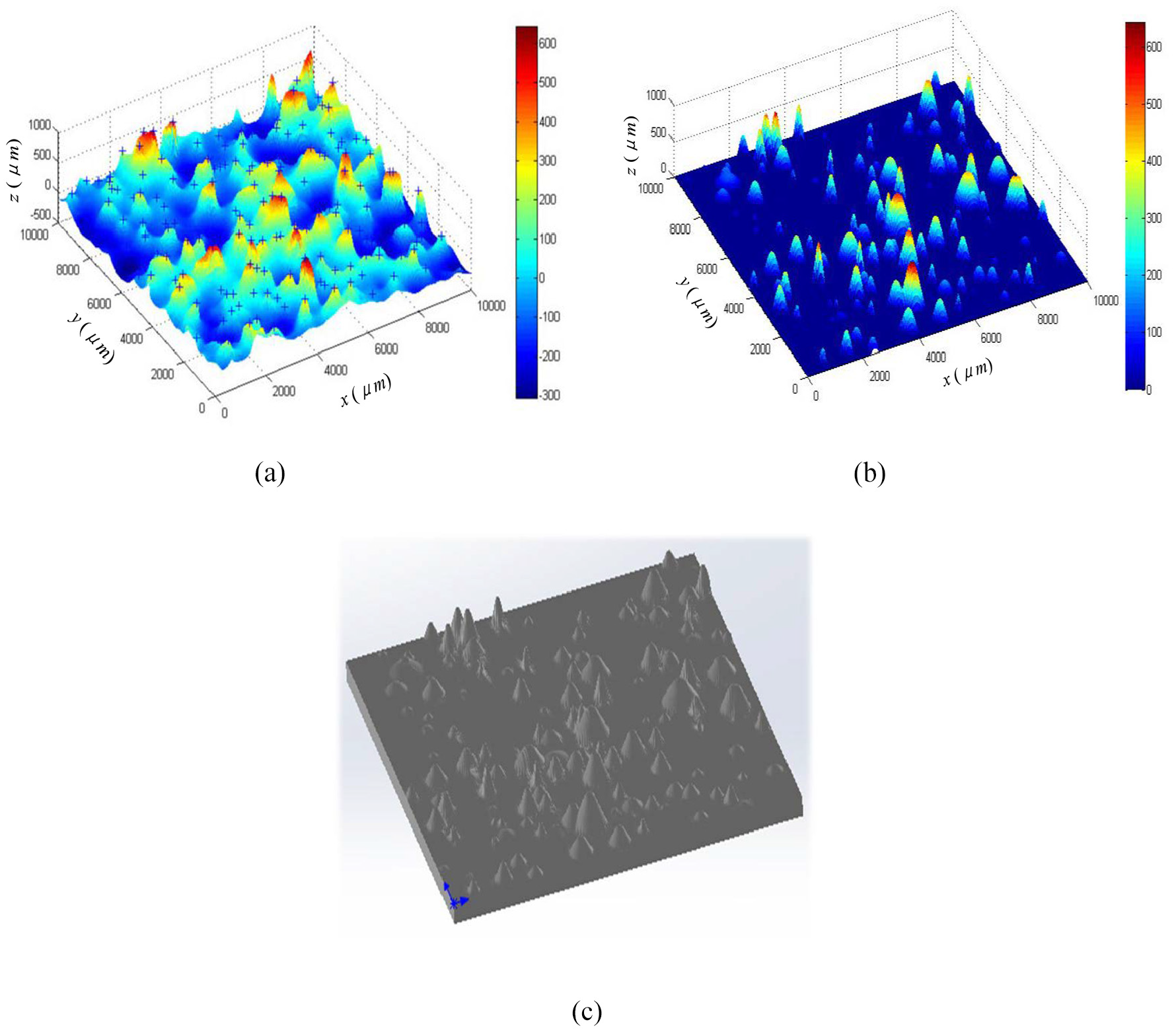
Digital representation of surface topography of abrasive belt. (a) Measured original topography. (b) Digitized feature topography. (c) 3D entity model.

Microscopic contact pressure model

The microscopic contact behavior and evolution process for abrasive belt rail grinding are shown in Figure 5. The contact case is modeled by setting the belt surface as rigid abrasive grits and the rail surface as elastic half-space. For the given total normal load F_N, the effective contact number of abrasive grits is constant. The shared load, the contact area and the invasion depth are different among active grits. Apparently, these parameters vary with F_N. The force balance equation always exists in the form below

F_{N} = \sum_{i = 1}^{n} F_{i}

(1)

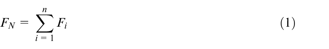
where F_i is the shared load for the ith active abrasive grit.

Figure 5.

Schematic diagram of the microscopic contact of abrasive belt grinding.

For the ith abrasive grit, the radius of the spherical end tip R_i and the attack angle α_i are used to define the geometrical shape. If the invasion depth d_i satisfies the condition d_i≤R_i(1−cosα_i), only the spherical end tip of the grit contacts the rail surface. Otherwise, the cone contact situation needs to be considered.

According to Hertzian contact theory,³⁷ the solution for the contact between a sphere and a plane is obtained as follows

F_{i} = \frac{4}{3} E^{*} R_{i}^{1 / 2} d_{i}^{3 / 2}

(2)

a_{i}^{2} = R_{i} d_{i}

(3)

A_{i} = π a_{i}^{2} = π R_{i} d_{i}

(4)

p_{i} = \frac{F_{i}}{A_{i}} = \frac{4 E^{*} d_{i}^{1 / 2}}{3 π R_{i}^{1 / 2}}

(5)

\frac{1}{E^{*}} = \frac{1 - v_{1}^{2}}{E_{1}} + \frac{1 - v_{2}^{2}}{E_{2}}

(6)

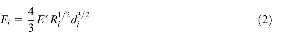
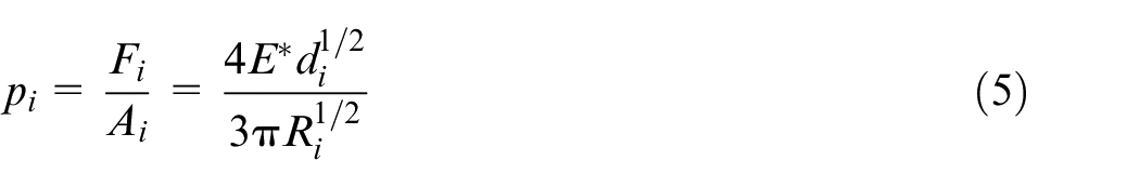
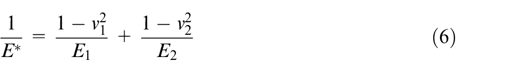
where α_i is the radius of the contact circle, A_i is the contact area, p_i is the equivalent stress, E* is the equivalent elastic modulus, E₁ and E₂ are, respectively, the elastic moduli of the abrasive grit and the rail surface and ν₁ and ν₂ are, respectively, the Possion’s ratios of the abrasive grit and the rail surface.

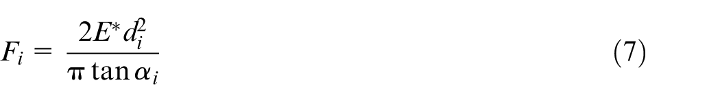
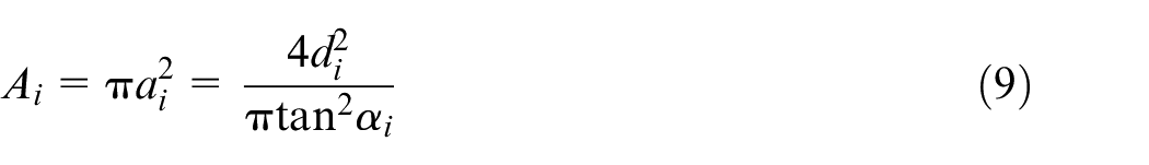
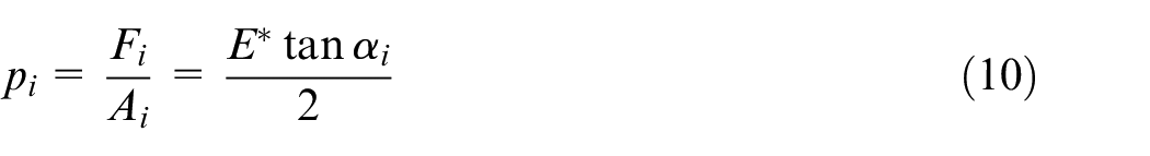
Similarly, for the cone contact, the following equations can be used³⁷

F_{i} = \frac{2 E^{*} d_{i}^{2}}{π \tan α_{i}}

(7)

a_{i} = \frac{2 d_{i}}{π \tan α_{i}}

(8)

A_{i} = π a_{i}^{2} = \frac{4 d_{i}^{2}}{π \tan^{2} α_{i}}

(9)

p_{i} = \frac{F_{i}}{A_{i}} = \frac{E^{*} \tan α_{i}}{2}

(10)

The microscopic contact pressure model based on grits can be expressed as

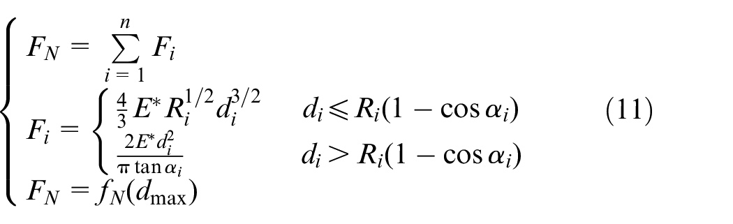
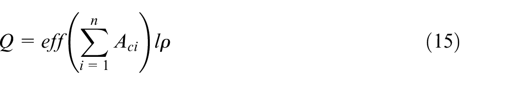
{\begin{matrix} F_{N} = \sum_{i = 1}^{n} F_{i} \\ F_{i} = {\begin{matrix} \frac{4}{3} E^{*} R_{i}^{1 / 2} d_{i}^{3 / 2} d_{i} \leq R_{i} (1 - \cos α_{i}) \\ \frac{2 E^{*} d_{i}^{2}}{π \tan α_{i}} d_{i} > R_{i} (1 - \cos α_{i}) \end{matrix} \\ F_{N} = f_{N} (d_{max}) \end{matrix}

(11)

where d_max is the maximum invasion depth of all active abrasive grits and f_N is the inherent functional relation equation between F_N and d_max.

Apparently, the numerical iterative method can be adopted to solve the above equations. The corresponding flow chart is shown in Figure 6. The characteristic parameters of rail and abrasive belt as well as the given total normal load F_N were chosen as the input parameters. When the sum of shared load ∑F_i for all active abrasive grits satisfies the inequality|(∑F_i)−F_N|< ε (ε is the iterative precision control parameter and ε > 0), the iterative process terminates and the microscopic contact behavior described with the shared load F_i, the contact area A_i and the equivalent stress p_i for every active abrasive grit can be obtained.

Figure 6.

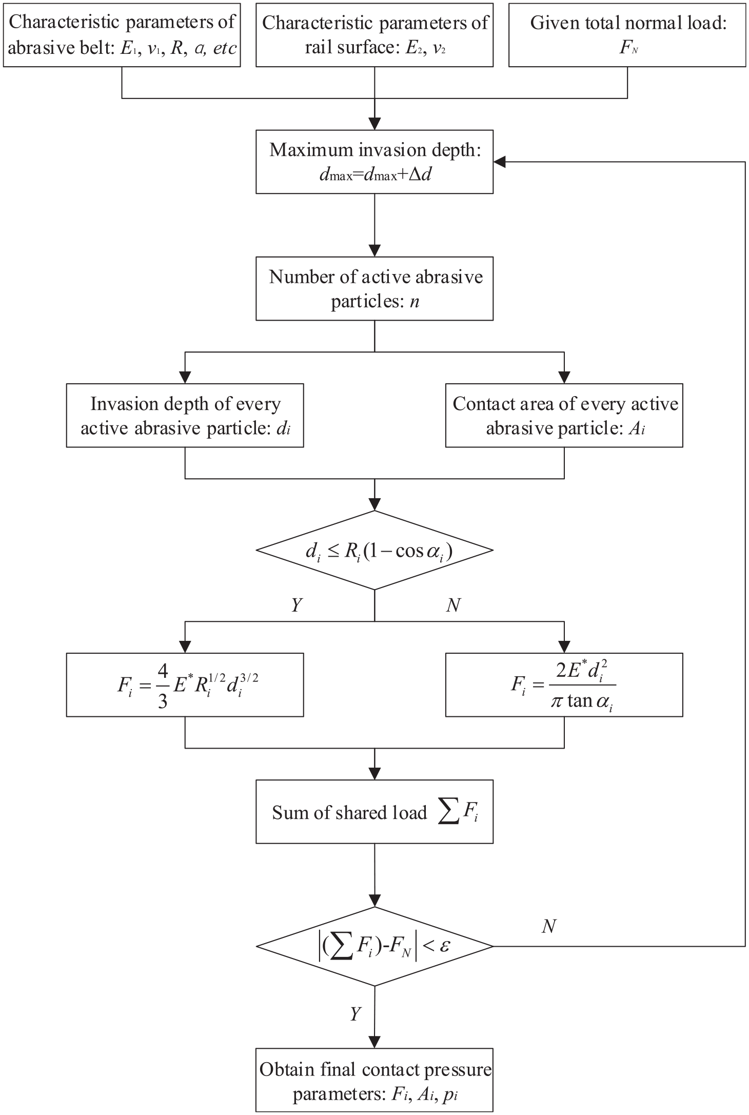
Flow chart of numerically solving the microscopic contact pressure model.

Material removal quantity model

In fact, the material removal process for rail grinding using abrasive belt is always associated with the compound cutting action generated by active grits in the contact area. Therefore, the microscopic cutting behavior of single grit is a key foundation for revealing the macro material removal mechanism. Figure 7 shows two cases with different section area constitutions for the ith abrasive grit under different invasion depths d_i. Obviously, when d_i≤R_i(1−cosα_i) holds, the section area A_ci is only related to the spherical end tip of the grit. Otherwise, the section area A_ci is composed of A_ci₁ and A_ci₂, which are, respectively, corresponding to the spherical end tip and the cone of abrasive grit.

Figure 7.

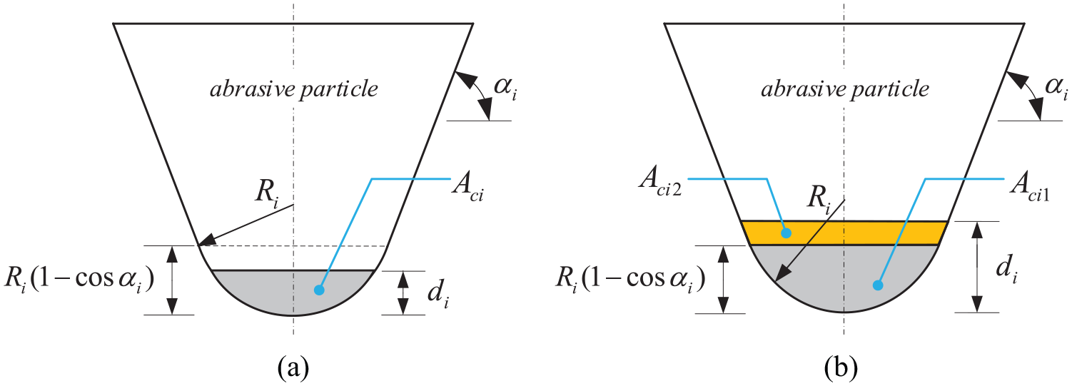
Two cases with different section area constitutions for the ith abrasive grit. (a) d_i≤R_i(1−cosα_i). (b) d_i>R_i(1−cosα_i).

As for the first case, based on the geometrical relationship, A_ci can be defined as

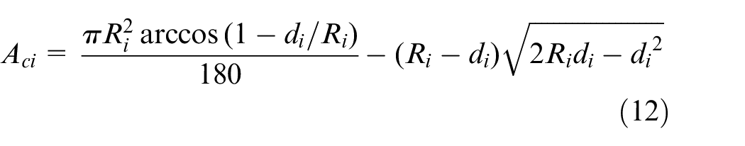
A_{ci} = \frac{π R_{i}^{2} \arccos (1 - d_{i} / R_{i})}{180} - (R_{i} - d_{i}) \sqrt{2 R_{i} d_{i} - {d_{i}}^{2}}

(12)

Particularly, when d_i = R_i(1−cosα_i) holds, A_ci can be expressed as

A_{ci} = \frac{π R_{i}^{2} α_{i}}{180} - R_{i}^{2} \sin α_{i} \cos α_{i}

(13)

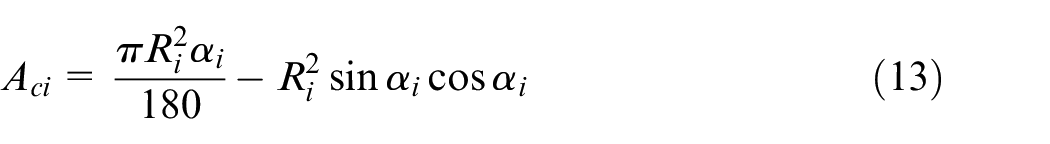
Similarly, A_ci for the second case can be given as

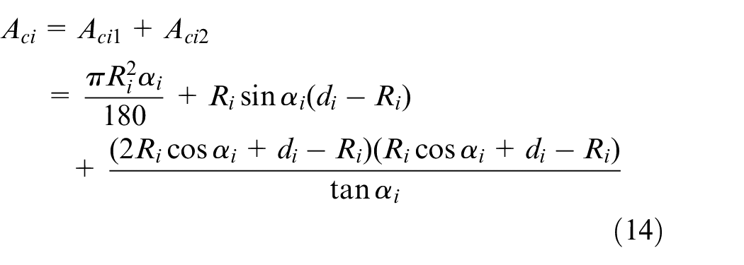
\begin{matrix} A_{ci} = A_{ci 1} + A_{ci 2} \\ = \frac{π R_{i}^{2} α_{i}}{180} + R_{i} \sin α_{i} (d_{i} - R_{i}) \\ + \frac{(2 R_{i} \cos α_{i} + d_{i} - R_{i}) (R_{i} \cos α_{i} + d_{i} - R_{i})}{\tan α_{i}} \end{matrix}

(14)

The interaction between grits should be considered to obtain the more accurate material removal quantity. Figure 8 shows the schematic diagram for calculating the material removal quantity. The characteristic horizontal contour curve formed by grits in the contact area can be extracted. Finally, for the given maximum invasion depth d_max, the material removal amount Q can be defined by

Q = eff (\sum_{i = 1}^{n} A_{ci}) l ρ

(15)

where the function eff represents the total effective section area, l is the longitudinal length of contact area and ρ is the rail density.

Figure 8.

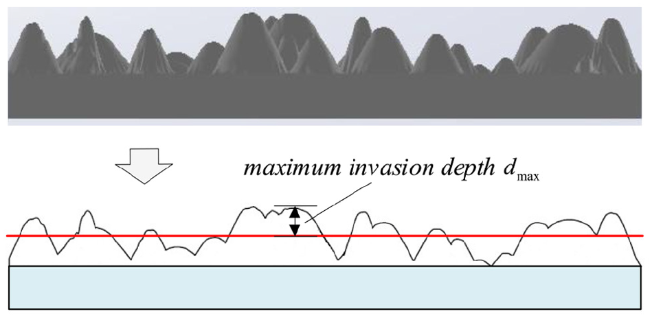
Schematic diagram for calculating the material removal quantity with the contour curve of abrasive grits.

Simulation and experimental verification

Comparative analysis of theoretical and simulation results of microscopic contact pressure

In this work, the VSM-40 ceramic abrasive belt with the size of 5 × 6 mm² was randomly chosen. According to the digital representation method, its main geometrical characteristic of surface topography referring to all the grits can be quantitatively extracted, and the corresponding 3D entity model can be rebuilt for the FE simulation, as shown in Figure 9. The physical parameters of the abrasive belt are E₁ = 350 GPa and v₁ = 0.22.

Figure 9.

Entity model for the selected VSM-40 ceramic abrasive belt.

The material chosen for the rail is AlSI4340 steel, which has mechanical properties: E₂ = 208 GPa and v₂ = 0.32. The FE simulation model was established by the ABAQUS software to analyze the microscopic contact behavior between abrasive grits and the rail surface. The meshing result is shown in Figure 10. In fact, the grits slid slightly on the contact surface because of the unavoidable deformation. The contact between abrasive grits and the rail surface was defined as the “small slip,” and the slip tolerance was set to be 0.006 mm.

Figure 10.

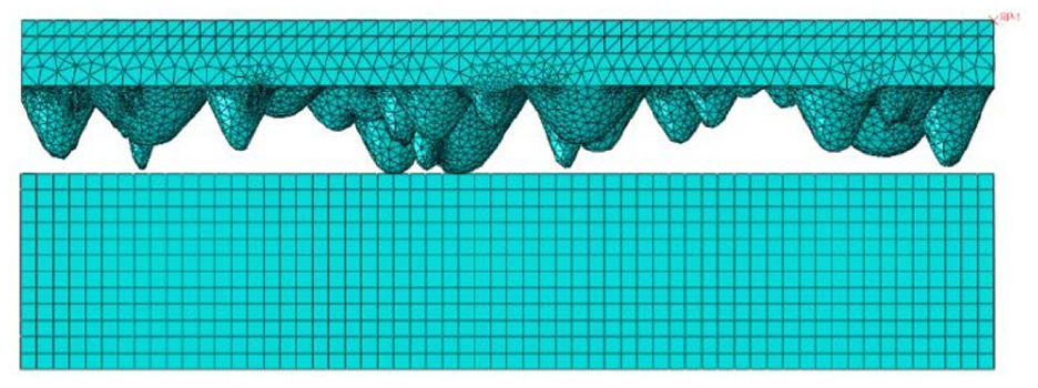
Meshing result of the FE simulation model.

As for the given series of normal loads applied on the back of the belt, the theoretical and simulation results of contact stress distribution of active grits are shown in Figure 11 and the theoretical results calculated with equation (11) are shown in the left column. The number N of active grits increased, when the normal load F_N discretely varied from 7 N to 115 N. Although the number N remained unchanged, the total contact area between the active grits and the rail surface was visibly enlarged significantly due to the increase in the normal load F_N, (Figure 11(b) and (c)). More importantly, in the evolution process of the above contact behavior, the theoretical results of the number and distribution of active grits are consistent with simulation results.

Figure 11.

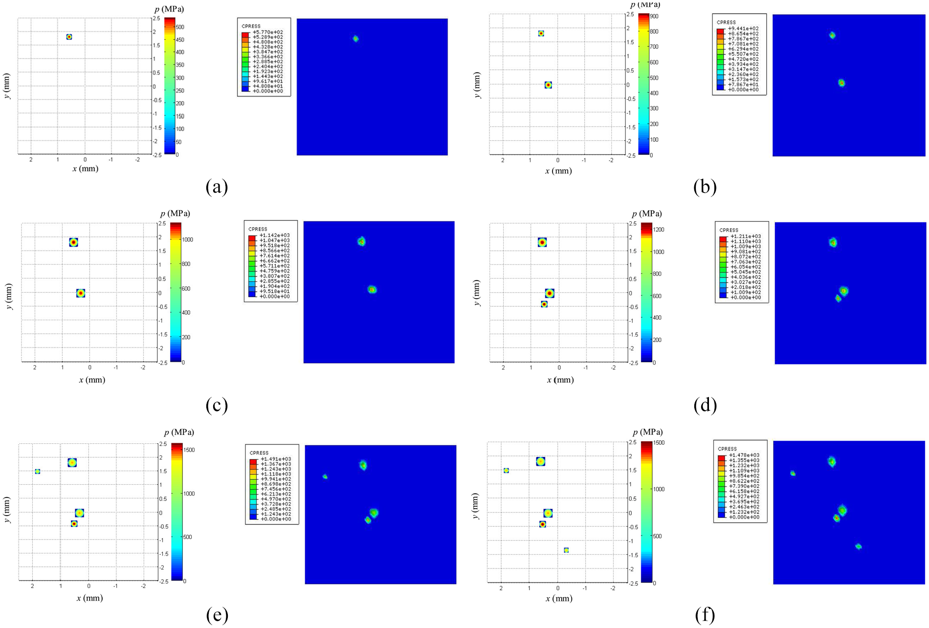
Theoretical and simulation results of contact stress distribution. (a) F_N = 7 N. (b) F_N = 36 N. (c) F_N = 67 N. (d) F_N = 80 N. (e) F_N = 100 N. (f) F_N = 115 N.

Afterward, the results of maximum contact stress obtained by the theoretical and FE simulation models are contrastively plotted in Figure 12. Overall, the maximum contact stress gradually became larger with the increase in the normal load F_N. At the early loading stage, the increasing trend of the maximum contact stress was obvious. However, when F_N > 100 N, the maximum contact stress became stable because the maximum contact stress had reached the yield stress of the material. Besides, the error caused by the necessary simplification of the theoretical and FE simulation models was inevitable and the maximum error was about 12% when F_N = 7 N. As expected, the theoretical results were mainly consistent with the simulation results under the given conditions.

Figure 12.

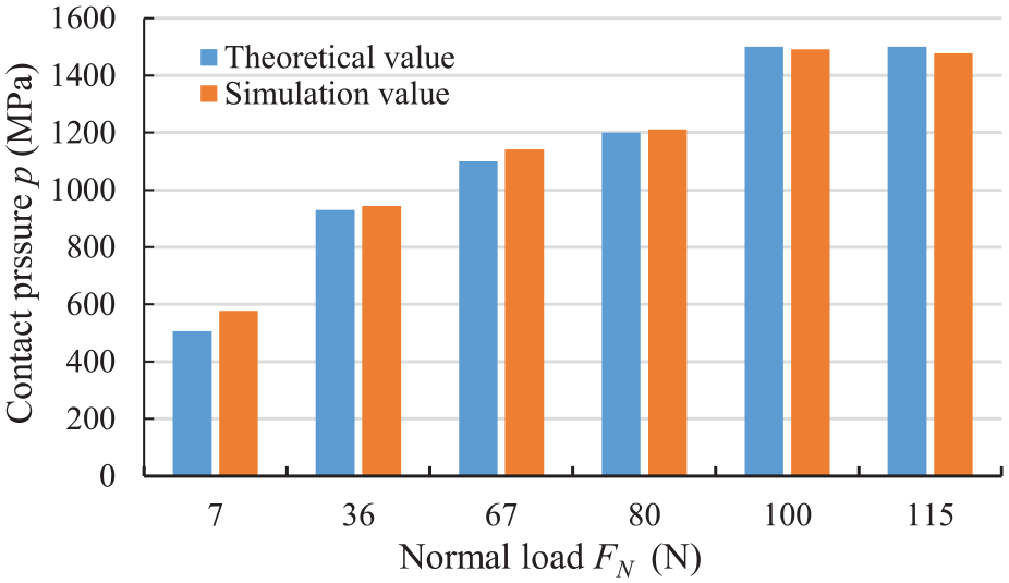
Theoretical and simulation results of maximum contact stresses.

Effect analysis of the abrasive belt topography on the contact stress

Three types of abrasive belt, corresponding to VSM-24, VSM-40 and VSM-60, were chosen as the research object. The required geometrical characteristics of grits and the reconstructed 3D entity models could be obtained in the same way mentioned above. The normal load F_N was, respectively, set as 5 N, 10 N, 15 N, 20 N, 25 N and 30 N. Figure 13 shows FE simulation results of the contact stress distribution for the three kinds of abrasive belts when F_N = 5 N.

Figure 13.

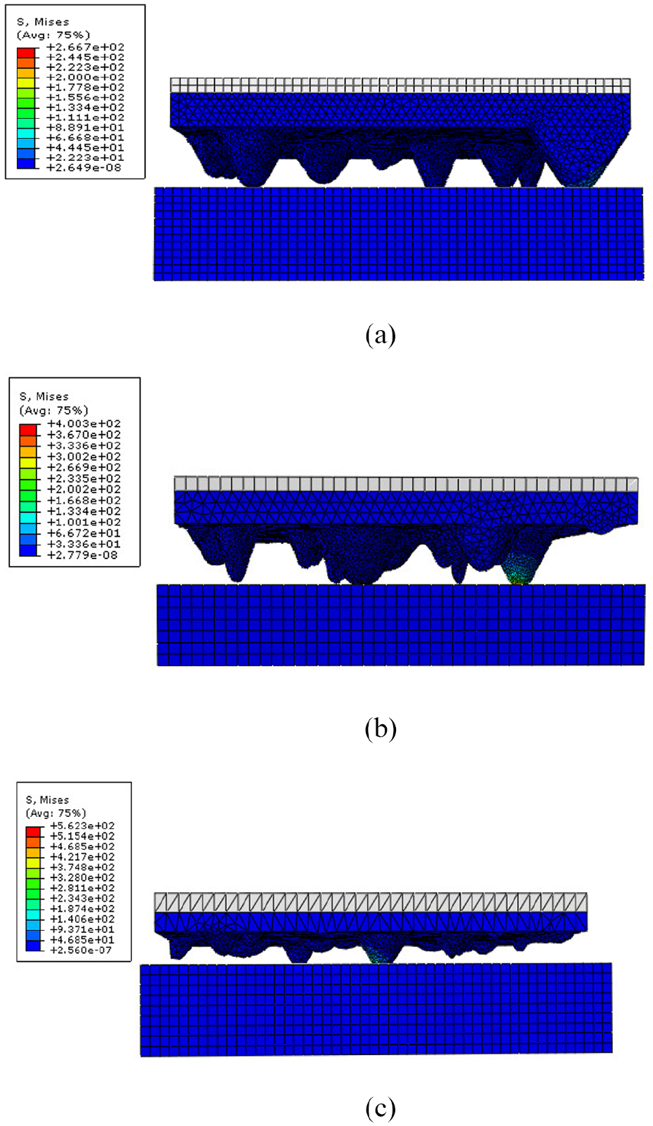
Simulation results of contact stresses distribution (F_N = 5 N). (a) VSM-24. (b) VSM-40. (c) VSM-60.

Similarly, the theoretical and simulation results of the contact stress for abrasive belts are contrastively plotted in Figure 14. The contact stress showed an upward trend along with the increase in the normal load F_N. However, the increasing rate gradually declined. The contact stress for VSM-60 was the largest, whereas that for VSM-24 was the smallest. The difference might be interpreted as follows. The stress reduction effect caused by the largest abrasive size and contact area of VSM-24 outweighed the stress enhancement effect caused by the minimal number of effective contact grits. In addition, the theoretical results and the simulation results for the three types of abrasive belts were almost the same and the maximum errors were, respectively, 11.2% (VSM-24), 9.0% (VSM-40) and 5.7% (VSM-60). The results indicated the consistency between the proposed theoretical model and the FE simulation model.

Figure 14.

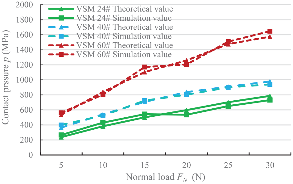
Theoretical and simulation results of the contact pressure.

Comparative analysis of theoretical and experimental results of material removal quantity

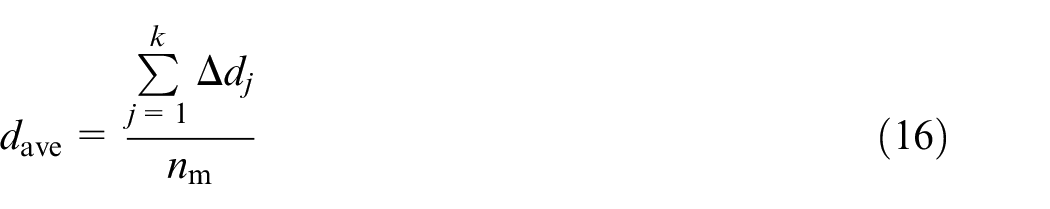
According to the models established above, the local contact load F_N on each small abrasive belt should be defined to calculate the material removal quantity. In this article, F_N was extrapolated with the previous method³⁸ to calculate the contact stresses for the grinding at any position and posture. To verify the proposed material removal quantity model, a series of grinding tests were conducted on the special experimental platform for rail grinding using abrasive belt (Figure 15). Furthermore, LK-H055 laser displacement sensor from Keyence was used to obtain the relative change in the radial height along the center line of the rail surface. The parameters of LK-H055 sensor are provided as follows: a measurement range of ± 5 mm, repeatability of 0.025 μm, a measurement resolution of 1 μm and a sampling frequency of 500 Hz. Total grinding cycles of n_m were collected for each grinding. LK-H055 totally captured k measurement points on the centerline of the rail surface. The height change at each measurement point is Δd_j, and j is the number of measurement points. The depth d_ave (μm/r) is expressed as

d_{ave} = \frac{\sum_{j = 1}^{k} Δ d_{j}}{n_{m}}

(16)

Figure 15.

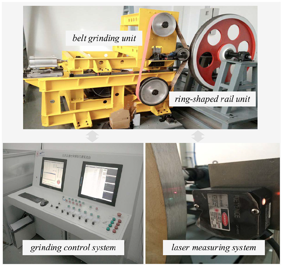
Special experimental platform for rail grinding using abrasive belt.

Therefore, the total mass loss Q_m can be calculated as

Q_{m} = π D_{R} ρ B_{R} d_{ave}

(17)

where D_R is the average diameter and B_R is the average width of the rail ring.

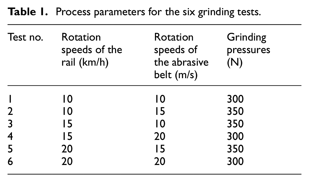
Six grinding tests with the random combinations of parameters based on the VSM-40 ceramic abrasive belt were planned and implemented. The main experimental parameters are listed in Table 1. The theoretical and experimental results of the material removal quantity in the six grinding tests are contrastively plotted in Figure 16. Theoretical results were well consistent with experimental results. The error values of the six grinding tests were 1.8%, 2.9%, 3.3%, 2.3%, 3.0% and 4.6%, respectively. The above results indicated that the industrial application of rail grinding using abrasive belt was feasible. However, the proposed material removal quantity model was verified to a certain degree and showed the application value of the abrasive belt rail grinding.

Table 1.

Process parameters for the six grinding tests.

Test no.	Rotationspeeds of the rail (km/h)	Rotationspeeds of the abrasivebelt (m/s)	Grinding pressures(N)
1	10	10	300
2	10	15	350
3	15	10	350
4	15	20	300
5	20	15	350
6	20	20	300

Figure 16.

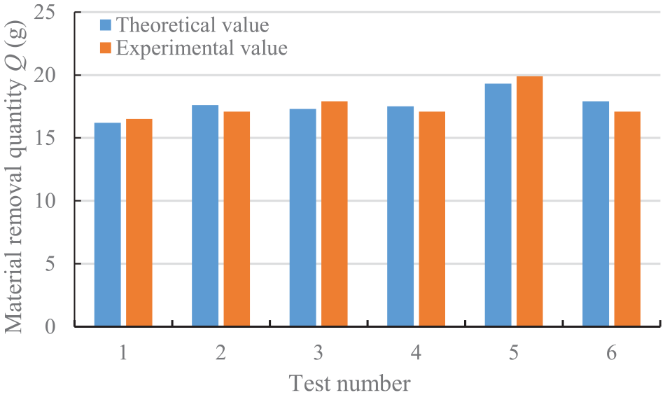
Theoretical and experimental results of the material removal quantity.

Conclusion

To understand the microscopic contact behavior between the rail surface and the abrasive belt, the representation of the abrasive belt topography was first realized in this study. The geometry of single abrasive grit was described as a cone with a spherical end tip and quantified with three indices: position, height and attack angle. The microscopic contact pressure model was proposed based on the abrasive belt surface and the contact behavior evolution process. Through the comparative analysis of theoretical and simulation results, the microscopic contact pressure model was verified to a certain degree. The results revealed the significant influence of the normal load and the abrasive belt topography on the microscopic contact behavior. A numerical model of material removal quantity was developed based on the characteristics of grits and their interactions. Six practical tests with the random combinations of parameters were implemented. The results effectively verified the theoretical model.

Footnotes

Declaration of conflicting interests

The author(s) declared no potential conflicts of interest with respect to the research, authorship, and/or publication of this article.

Funding

The author(s) disclosed receipt of the following financial support for the research, authorship, and/or publication of this article: The study was financially supported by the Fundamental Research Funds for the Central Universities (Grant No. 2019JBM050).

ORCID iDs

Wengang Fan

Wenxi Wang

References

Cannon

Edel

Grassie

, et al. Rail defects: an overview. Fatigue Fract Eng Mater Struct 2003; 26: 865–886.

Steenbergen

. Rolling contact fatigue in relation to rail grinding. Wear 2016; 356–357: 110–121.

Eric

Joseph

. The application of contact mechanics to rail profile design and rail grinding. Wear 2002; 253: 308–316.

Zhi

Zarembski

. Towards a better understanding of the rail grinding mechanism. In: Proceedings of the ASME 2013 rail transportation division fall technical conference, Altoona, PA, 15–17 October 2013. New York: ASME.

Real

Zamorano

Velarte

, et al. Development of a vehicle–track interaction model to predict the vibratory benefits of rail grinding in the time domain. J Mod Transp 2015; 23(3): 189–201.

Cuervo

Santa

Toro

. Correlations between wear mechanisms and rail grinding operations in a commercial railroad. Tribol Int 2015; 82: 265–273.

Lin

Wang

, et al. Analysis on the effects of rotational speed of grinding stone on removal behavior of rail material. Wear 2015; 342–343: 52–59.

Zhi

Zarembski

. Grinding motor energy saving method based on material removal model in rail grinding processes. Int J Pr Eng Man: Gt 2015; 2(1): 21–30.

Santa

Toro

Lewis

. Correlations between rail wear rates and operating conditions in a commercial railroad. Tribol Int 2016; 95: 5–12.

10.

Zhang

Shang

Ding

, et al. Thermal model and temperature field in rail grinding process based on a moving heat source. Appl Therm Eng 2016; 106: 855–864.

11.

Zhang

, et al. Probing the effect of abrasive grit size on rail grinding behaviors. J Manuf Process 2020; 53: 388–395.

12.

Singleton

Marshall

Lewis

, et al. Rail grinding for the 21st century—taking a lead from the aerospace industry. Proc IMechE, Part F: J Rail and Rapid Transit 2014; 229(5): 457–465.

13.

Uhlmann

Lypovka

Hochschild

, et al. Influence of rail grinding process parameters on rail surface roughness and surface layer hardness. Wear 2016; 366–367: 287–293.

14.

Linsinger. https://www.linsinger.com/rail-processing/ (accessed 20 June 2019).

15.

Vossloh. https://www.vossloh.com/en/products-and-solutions/products-at-a-glance/rail-turnouts.maintenance/ (accessed 20 June 2019).

16.

Liu

, et al. Investigating the effects of contact pressure on rail material abrasive belt grinding performance. Int J Adv Manuf Tech 2017; 93(1–4): 779–786.

17.

Xiao

Huang

Liu

, et al. Analysis of vibration from low-rigidity contact in belt grinding of blisk blade. Proc IMechE, Part B: J Engineering Manufacture 2019; 233(12): 2345–2357.

18.

Vigneashwara

Wahyu

Tegoeh

, et al. In-process tool condition monitoring in compliant abrasive belt grinding process using support vector machine and genetic algorithm. J Manuf Process 2018; 31: 199–213.

19.

Wang

Zhang

, et al. An investigation of surface corrosion behavior of Inconel 718 after robotic belt grinding. Materials 2018; 11(12): 2440.

20.

Wang

, et al. A comprehensive study on surface integrity of nickel-based superalloy Inconel 718 under robotic belt grinding. Mater Manuf Process 2019; 34(1): 61–69.

21.

Zhang

, et al. Modeling and prediction of surface roughness in belt polishing based on artificial neural network. Proc IMechE, Part B: J Engineering Manufacture 2018; 232(12): 2154–2163.

22.

Vigneashwara

Pushparaja

Tegoeh

, et al. In-process verification of weld seam removal in robotic abrasive belt grinding process using deep learning. Robot Cim: Int Manuf 2019; 31: 477–487.

23.

Huang

Xiao

, et al. Effects research on theoretical-modelling based suppression of the contact flutter in blisk belt grinding. J Manuf Process 2020; 54: 309–317.

24.

Huang

Jiahua

Xiao

, et al. Study on the surface topography of the vibration-assisted belt grinding of the pump gear. Int J Adv Manuf Tech 2020; 106(1–2): 719–729.

25.

Sun

Halil

, et al. Pressure distribution of serrated contact wheels—experimental and numerical analysis. Int J Adv Manuf Tech 2017; 90: 3407–3419.

26.

Fan

Liu

Song

, et al. Influencing mechanism of rubber wheel on contact pressure and metal removal in corrugated rail grinding by abrasive belt. J Manuf Sci E: T ASME 2018; 140: 124501.

27.

Wang

Fan

. Investigation into static contact behavior in belt rail grinding using a concave contact wheel. Int J Adv Manuf Tech 2019; 101: 2825–2835.

28.

Jourani

Hagege

Bouvier

, et al. Influence of abrasive grain geometry on friction coefficient and wear rate in belt finishing. Tribol Int 2013; 59: 30–37.

29.

Khellouki

Rech

Zahouani

. Micro-scale investigation on belt finishing cutting mechanisms by scratch tests. Wear 2013; 308: 17–28.

30.

Subramanian

Babu

Jain

, et al. Microscopic interactions in surface generation processes using abrasive tools. J Manuf Sci E: T ASME 2017; 139(12): 121016.

31.

Jourani

. A new three-dimensional numerical model of rough contact: influence of mode of surface deformation on real area of contact and pressure distribution. J Tribol: T ASME 2015; 137: 011401.

32.

Wang

Fan

, et al. Characteristic quantitative evaluation and stochastic modeling of surface topography for zirconia alumina abrasive belt. Int J Adv Manuf Tech 2017; 89(9–12): 3059–3069.

33.

Zhang

Wang

Kang

, et al. Changes in surface layer of silicon wafers from diamond scratching. CIRP Ann: Manuf Techn 2015; 64(1): 349–352.

34.

Wang

Zhang

Chang

, et al. New deformation-induced nanostructure in silicon. Nano Lett 2018; 18(7): 4611–4617.

35.

Zhang

Huang

Wang

, et al. A novel approach of high-performance grinding using developed diamond wheels. Int J Adv Manuf Tech 2017; 91(9–12): 3315–3326.

36.

Zhang

Wang

, et al. Nanoscale wear layers on silicon wafers induced by mechanical chemical grinding. Tribol Lett 2017; 65(4): 132.

37.

Valentin

. Rigorous treatment of contact problems—Hertzian contact. In: Valentin

(ed.) Contact mechanics and friction: physical principles and applications. 1st ed. Berlin: Springer, 2017, pp.55–70.

38.

Wang

Fan

, et al. A numerical model to investigate contact status for rail grinding by abrasive belt with an axial deflection. J Braz Soc Mech Sci 2019; 41(11): 494.

Microscopic contact pressure and material removal modeling in rail grinding using abrasive belt

Abstract

Keywords

Introduction

Microscopic contact pressure model

Digital representation of the surface topography of abrasive belt

Microscopic contact pressure model

Material removal quantity model

Simulation and experimental verification

Comparative analysis of theoretical and simulation results of microscopic contact pressure

Effect analysis of the abrasive belt topography on the contact stress

Comparative analysis of theoretical and experimental results of material removal quantity

Conclusion

Footnotes

Declaration of conflicting interests

Funding

ORCID iDs

References