
Abstract
To eliminate the disadvantages of linear interpolation and geometry-based smoothing methods, the one-step corner smoothing method with feedrate blending algorithm for linear segments is proposed in this article. In the proposed method, the variable acceleration and jerk optimization method will be first adopted to determine the dynamic performance of each linear segment for feedrate scheduling, which takes the different axial limits into consideration. Then, the feedrate scheduling method based on the S-type acceleration and deceleration algorithm is implemented to generate smooth feedrate profiles. Moreover, the feedrate blending algorithm is adopted to calculate the corner time analytically within the specified corner error and thus to generate the smooth trajectory without inserting a smooth curve at adjacent linear segments. With the presented one-step corner smoothing method, a smoother and more accurate trajectory could be generated with faster machining time. The results of simulations and machining experiments demonstrate the effectiveness of the proposed method.
Keywords
Introduction
In modern computer-aided design (CAD) system, smooth parametric splines such as nonuniform rational basis spline (NURBS) or B-splines are commonly used to design the free-form surfaces. However, due to the difficulties in parametric interpolation, the direct parametric interpolators have not been widely used in industrial computer numerical control (CNC) systems.1,2 Moreover, linear segments (G01) are still the most commonly used format to approximate the toolpaths in both the computer-aided manufacturing (CAM) and current industrial CNC systems.3,4 Nevertheless, the linear segments are only G0 continuity; as a consequence, the motion has to stop at the junctions to completely avoid the discontinuities of feedrate, acceleration, and jerk,2,5,6 which absolutely lead to longer machining time.
To achieve nonstop continuous motion, thus to improve the machining efficiency and quality, two major techniques—that is, global smoothing and corner smoothing techniques—have been proposed. 3 The global smoothing means that a portion of the linear toolpath is fitted to generate the continuous parametric toolpath. The corner smoothing method means that a smooth curve is inserted at the corner of two adjacent linear segments to achieve nonstop continuous motion. Generally, both two methods mentioned above contain two steps, curve fitting followed by feedrate scheduling. First, the linear segments will be smoothed by a parametric curve, such as Bezier,3,7 B-spline,4,8,9 or NURBS, 10 and the toolpath becomes parametric curves or a mixture of linear segments and parametric curves. Then, the feedrate scheduling will be applied to generate a smooth feedrate profile for real-time interpolation. However, it is inefficient to separate the smoothing method into curve fitting and feedrate scheduling. 2 In addition, the feedrate fluctuation is unavoidable due to the discrepancy between the spline parameter and the arc length 11 in parametric interpolation. Besides, it is time-consuming to accomplish the complicated computation of the parametric curve, 12 which will affect the real-time performance of CNC systems.
In order to eliminate the shortcomings for two-step smoothing methods, one-step local corner smoothing method,2,5,6,13–18 which blends the axial velocities directly, has become the research hotspot in the field of CNC interpolation. For instance, Huang 13 provided a blending feedrate planning method for both linear and S-curve acceleration and deceleration algorithms, by which the feedrate at both ends of two blocks will automatically be overridden with consideration of maximum corner error. This method can ensure that the feedrate variation of two blocks is continuous, and the end feedrate of previous block does not decelerate to zero. However, only the corner error is considered in the above-mentioned algorithm, and the dynamic constraints of individual axis are not paid attention to. He et al. 14 presented an algorithm to smooth the track and velocity by adding motion vectors of two adjacent segments. The algorithm can smooth linear segments according to the maximum corner error based on the trapezoidal velocity profile. However, only geometrical error was taken into consideration in the proposed method. Zhang et al. 5 proposed a multi-period algorithm to improve the transition feedrate at the corner based on the linear acceleration and deceleration mode. This method utilized the maximal acceleration capabilities of the CNC machines and significantly improved the cutting efficiency with satisfying the machining accuracy. However, with linear acceleration and deceleration approach, sudden changes of acceleration at the junction of two linear segments will occur. 16 Then, Zhang et al. 16 developed a new multi-period turning interpolation algorithm based on the S-curve control method, which improves the feedrate at the corner by inserting a cubic curve at the junction of two segments. With the proposed method, the machining vibration was decreased, and the machining quality was improved. However, this algorithm ignores the constant acceleration phase of S-curve control algorithm, which is only suitable for some special cases. Zhang et al. 15 used a one-step strategy to generate the transition trajectory based on the linear acceleration algorithm, which aims to minimize the total machining time with the maximal axial accelerations and error tolerance. However, sudden changes of acceleration still exit. Tajima and Sencer2,17 proposed the kinematic corner smoothing method for long linear segments, which plans the jerk-limited feedrate profiles directly around the segment junctions. This method can generate a continuous feed motion with precisely controlled contouring errors of corners. Then, Tajima and Sencer 6 and Du et al. 18 came up with a new global toolpath smoothing method for short linear segments with jerk-limited feedrate profile and jounce-limited feedrate profile, respectively, which blends the axis feedrate between consecutive linear toolpaths within limited corner errors and kinematic limits of drives. Both of the two above-mentioned corner smoothing techniques can eliminate the need for two-step geometric corner smoothing methods, and provide better contouring performance. However, the proposed methods are based on the assumption that cornering motion starts and ends with identical cornering feedrate and acceleration to generate symmetric trajectories around the corners, which limits the application in one-step corner smoothing for linear segments.
Thus, in this article, the one-step corner smoothing algorithm is proposed, where the linear segments are smoothed by blending the tangential feedrate from one segment to the other, based on the S-type acceleration and deceleration algorithm. The control of the smoothing corner error, axis acceleration, and axis jerk are tackled by simple and analytical methods. The advantages of the proposed algorithm are as follows: (1) with the one-step method, the corner error is directly constrained in an analytical way, which will also determine the corner time when the blending feedrate starts; (2) variable acceleration and jerk optimizations determine the jerk and acceleration for feedrate scheduling, which can generate continuous axial acceleration and limited axial jerk in corner smoothing process; (3) compared with the two-step corner smoothing method (TCM), a faster and smoother motion can be obtained around the corner without inserting a blending curve. Besides, the curve scanning, parameter calculation, and derivative computation of the parametric curve are eliminated by the proposed algorithm, which is more convenient to apply in real-time CNC systems. The rest of this article is organized in detail as follows. In section “Corner smoothing method with feedrate blending for linear segments,” the feedrate scheduling method and the feedrate blending algorithm for corner smoothing are presented. In section “Simulation and experiment,” simulation and experiment are conducted to compare different methods with the proposed algorithm. Finally, the conclusion of this article is described in section “Conclusion.”
Corner smoothing method with feedrate blending for linear segments
The whole architecture of the proposed corner smoothing method is shown in Figure 1, which is divided into two blocks. The former offline module aims to determine the parameters of constraints in feedrate scheduling, according to the target feedrate, limited axial acceleration, axial jerk, and corner error. Then, the latter real-time module will generate the smooth S-type feedrate profiles and determine the corner time under corner error constraint, and thus calculate the commanded position and generate the smoothed trajectory at the corner.
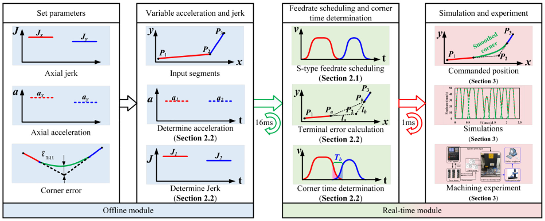
The flowchart of the proposed method.
Feedrate scheduling based on S-type acceleration and deceleration algorithm
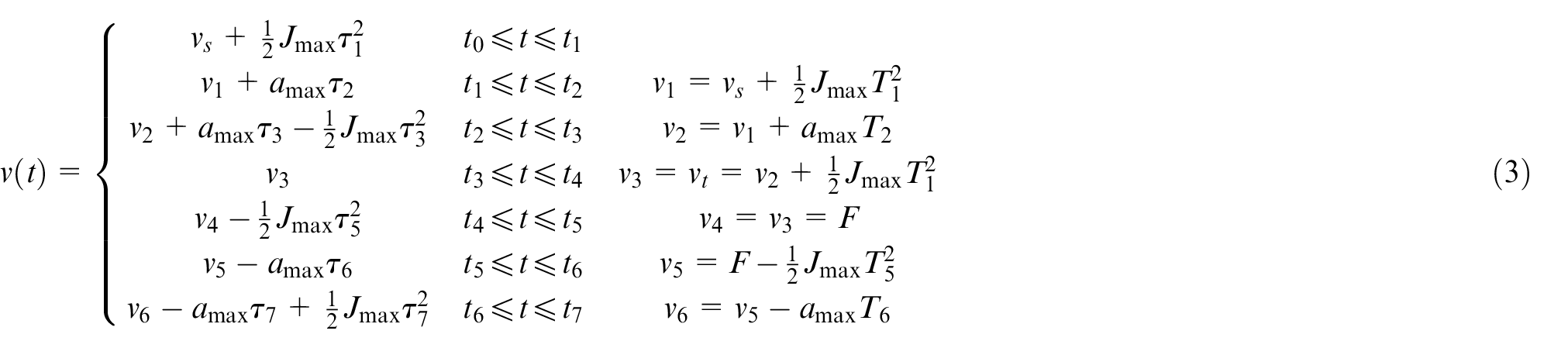
The S-type acceleration and deceleration algorithm is widely used in modern CNC systems,2,6,16,17,19–22 due to its stability and low computational burden. 23 As shown in Figure 2(a), the complete S-type acceleration and deceleration profile is usually divided into seven phases,19–22 including increasing acceleration (Phase I), constant acceleration (Phase II), decreasing acceleration (Phase III), constant feedrate (Phase IV), increasing deceleration (Phase V), constant deceleration (Phase VI), and decreasing deceleration (Phase VII). Furthermore, Phases I, II, and III are defined as the acceleration phase, meanwhile, Phases V, VI, and VII are defined as the deceleration phase.
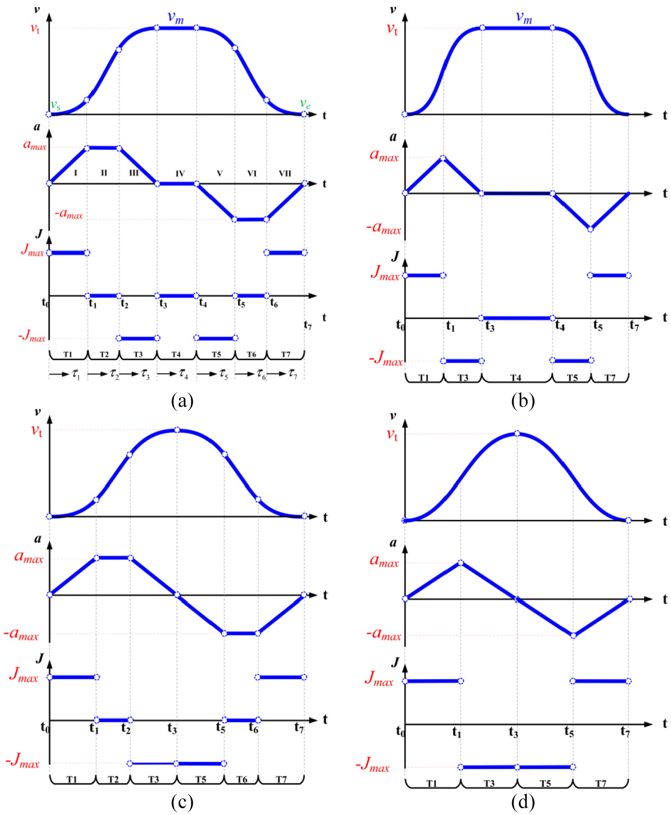
Four types of feedrate profiles: (a) type I, (b) type II, (c) type III, and (d) type IV.
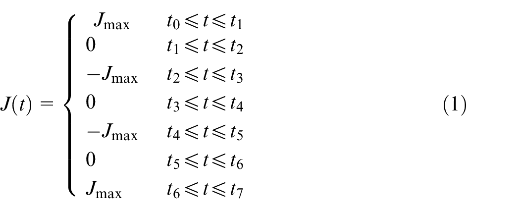
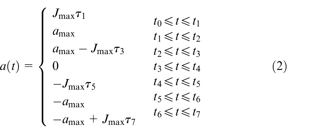
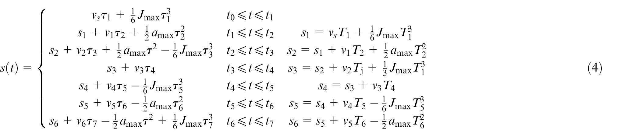
The expression of the jerk, the acceleration, the velocity, and the position are summarized below
In the feedrate scheduling, the maximum acceleration
If the initial values of the length of the segment
As mentioned above, to avoid the sudden change of acceleration, the machine usually comes to a full stop at junctions of linear segments with only position (G0) continuity, which means that in feedrate scheduling, starting feedrate and ending feedrate are equal to zero
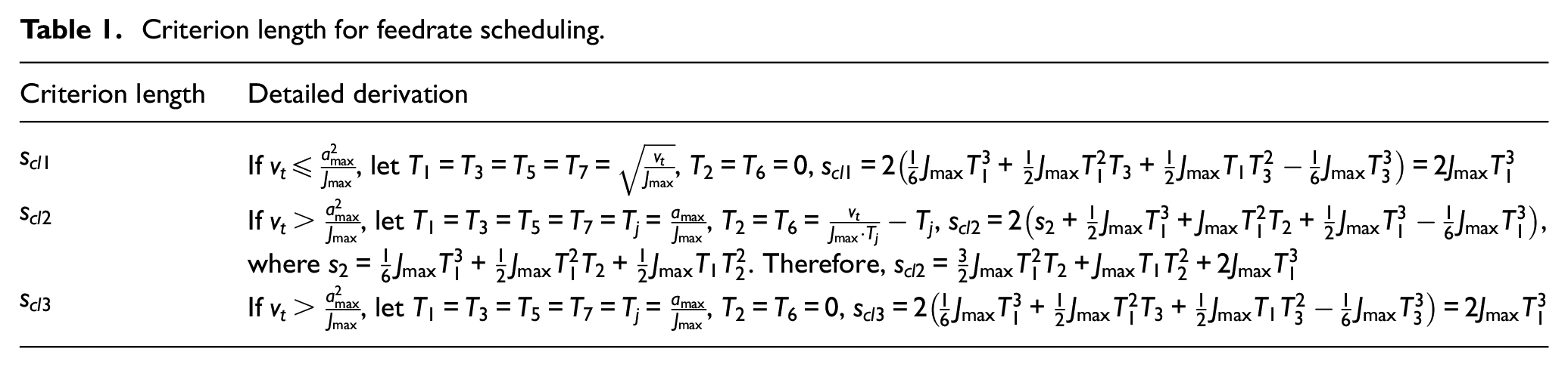
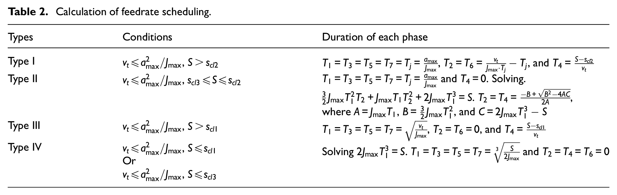
The criterion lengths for type determination and the durations of phases for each forward scheduling type are listed in Tables 1 and 2, respectively. Then, according to the relationship between
Criterion length for feedrate scheduling.
Calculation of feedrate scheduling.
Feedrate blending algorithm for linear segments
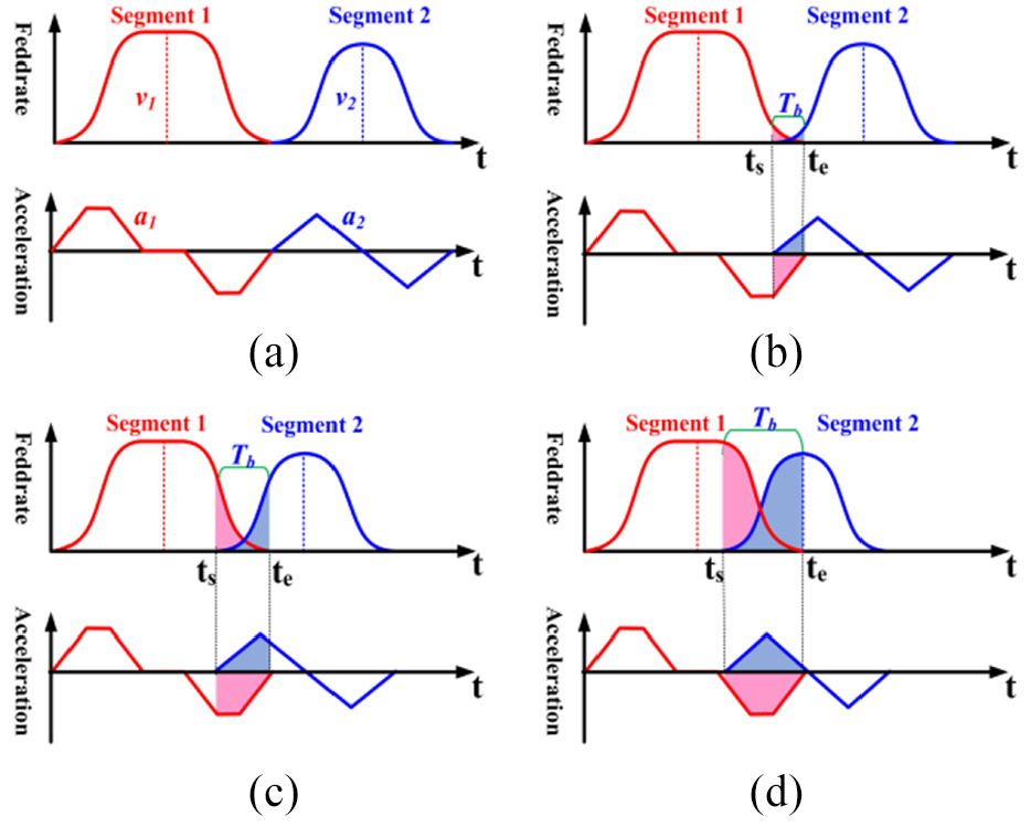
Based on the S-type acceleration and deceleration algorithm, the feedrate profile of each segment can be generated. As shown in Figure 3(a), there are two consecutive segments with different feedrate profiles. To improve the machining efficiency, when the first segment is decelerating and its feedrate is not zero, then the acceleration of second segment starts. Thus, the feedrate of two segments is blended in the time period
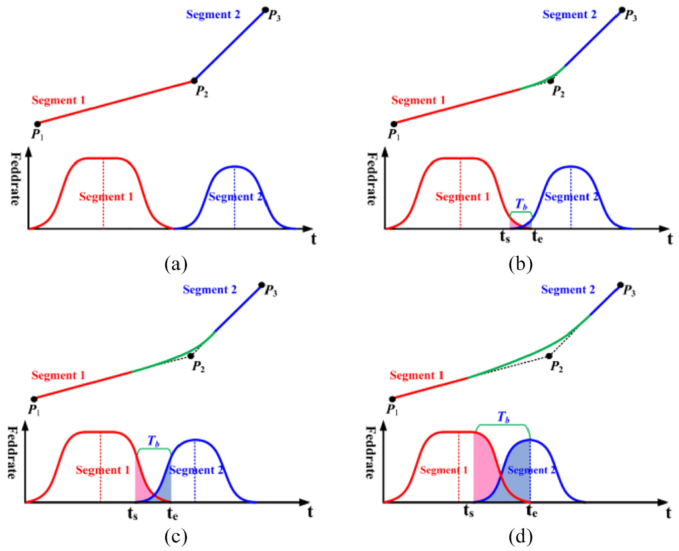
Different cases of feedrate blending: (a) case I, (b) case II, (c) case III, and (d) case IV.
Geometrical error control
As shown in Figure 4(a), the corner motion starts from point
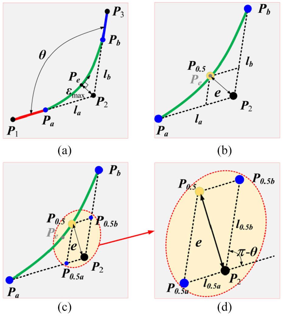
The corner error and terminal errors: (a) the definition of corner error and terminal error, (b) the corner error when the feedrate profile is symmetric, (c) the corner error when the feedrate is asymmetric, and (d) the relation of corner error and terminal error.
As shown in Figure 4(a), when the feedrate profiles are identical, the smoothed corner is symmetric around the corner bisector; hence, the maximum corner error

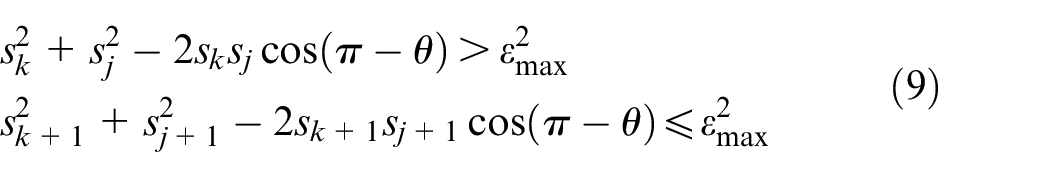
As a result, as long as the distance of
Supposing that

According to the S-type acceleration and deceleration algorithm, introduced in section “Feedrate scheduling based on S-type acceleration and deceleration algorithm,”
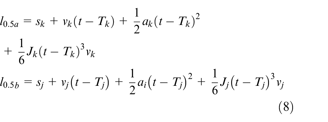
where
The values of
Thus, the following expression can be calculated by combining equations (7) and (8)
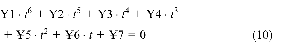
where
The time
where
Feedrate control in the blending process
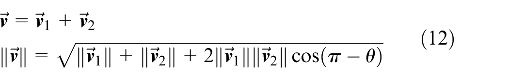
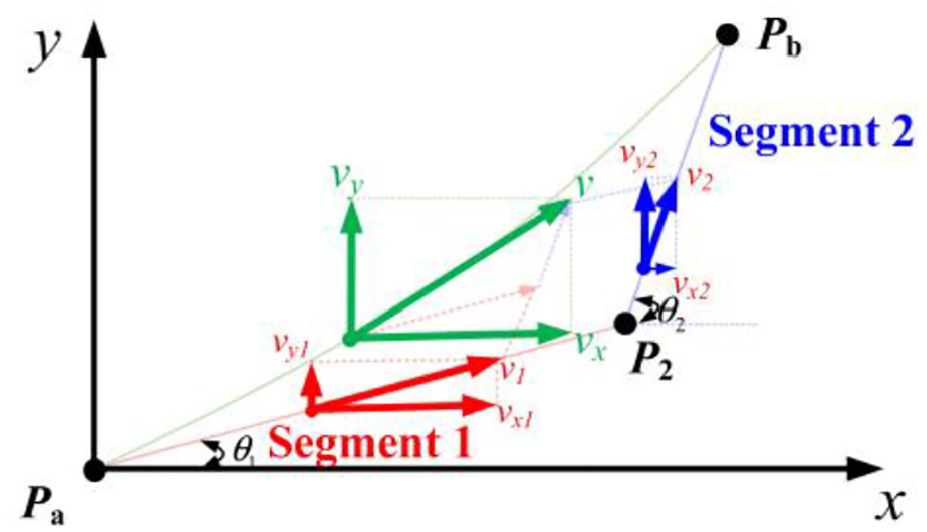
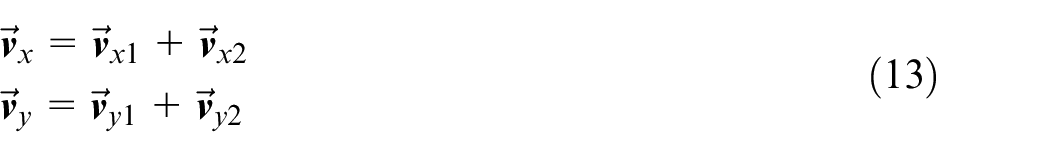
As shown in Figure 5(a), when the tool moves along the blending trajectory, the feedrate is defined as the norm of the addition of two velocity vectors, which can be expressed as equation (12). According to the algorithm of vector addition, it can be demonstrated that the feedrate reaches the maximum value when two velocity vectors are in the same direction, as depicted in Figure 5(b). Therefore, as long as the feedrate, generated by two velocity vectors with identical direction, could be controlled within the specified limits, the actual feedrate in the blending process would not exceed the allowable value
Vector addition of the feedrate: (a) the feedrate along the toolpath and (b) different situations of the vector addition.
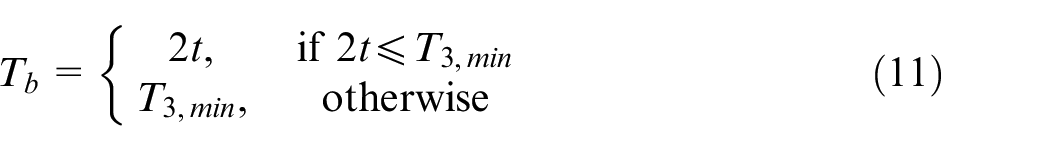
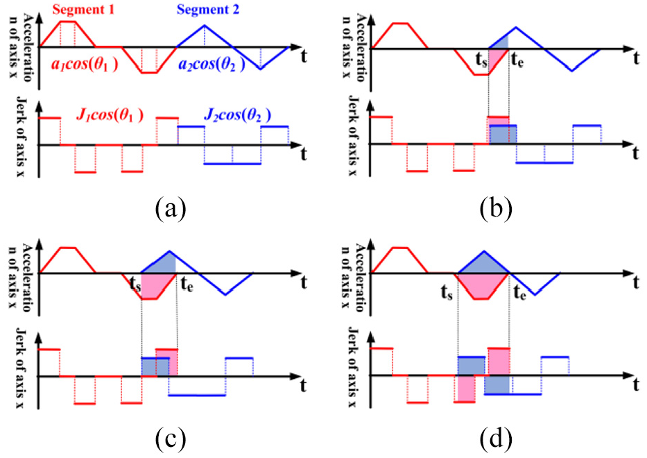
As mentioned above that the corner time is limited to no longer than the duration of deceleration phase of first segment or the duration of acceleration phase of second segment, therefore, the addition of the acceleration with the same direction will be negative first and then it becomes positive, as shown in Figure 6, which means that the feedrate, generated by two velocity vectors with identical direction, will decelerate first and then accelerate. As a result, the maximum feedrate in the blending process will occur at the start or the end. What’s more, since the corner time is limited to no longer than the durations of the first deceleration phase or the second acceleration phase, the feedrate will be controlled within the limited feedrate (constant feedrate phase), as shown in Figure 6. Therefore, the corner feedrate will be constrained within the programmed value by the proposed feedrate blending method (FBM).
The addition of the acceleration with the same direction: (a) case I, (b) case II, (c) case III, and (d) case IV.
Variable acceleration and jerk in feedrate scheduling
For machining process, the machining precision is influenced not only by the feedrate but also by the limited drive ability of the machine tool, including the axial acceleration and jerk. 1 Therefore, to avoid violating the capacities of each individual drive, the drive constraints in feedrate scheduling should be limited.
As Figure 7 depicts, the axial feedrate of the addition of two velocity vectors can be expressed as
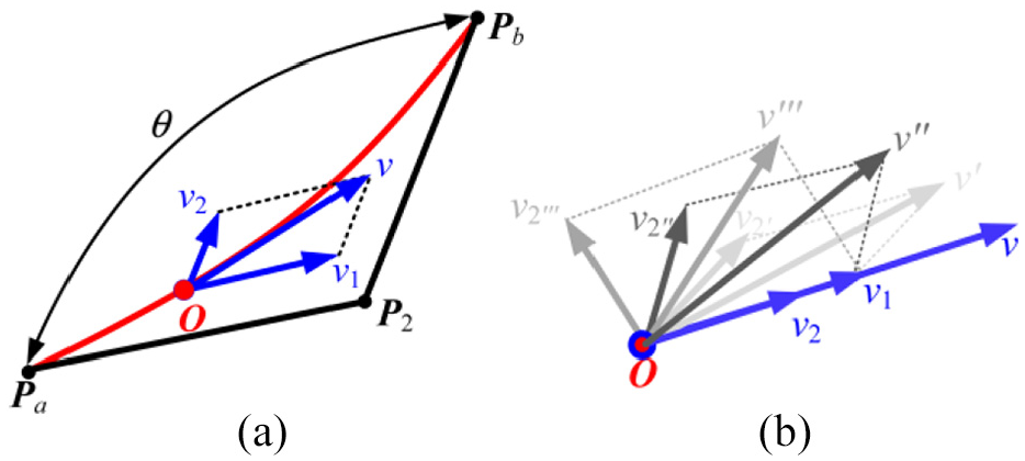
The addition of the axis feedrate.
Then, the following equation can be obtained by the algorithm of vector addition

As a result, the acceleration and the jerk of axes x and y in the blending process can be expressed
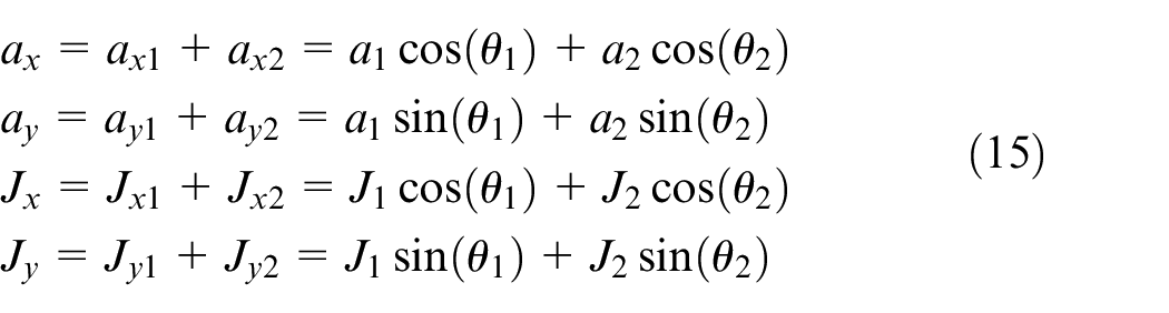
where
Acceleration selection for feedrate scheduling and axial limitation
The acceleration and the jerk of axes x and y, as shown in Figure 8, correspond to the feedrate profile shown in Figure 6(a). The possible situations of feedrate blending are presented in Figure 8. In the feedrate blending process,
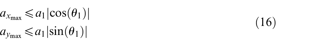
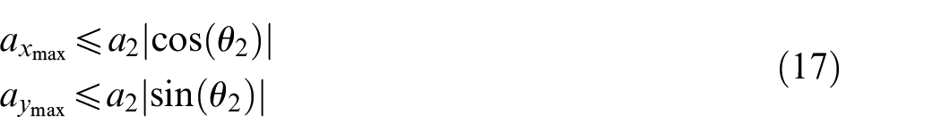
Different cases of additions of axis acceleration and jerk: (a) case I, (b) case II, (c) case III, and (d) case IV.
Therefore, the tangential acceleration amplitude used in feedrate scheduling can be determined by equation (18)
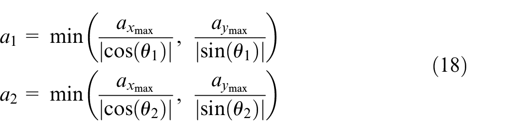
where
Optimal jerk determination to minimize the acceleration time
Figure 8(b) indicates the possible maximum axial jerk; therefore, if the tangential jerk
where
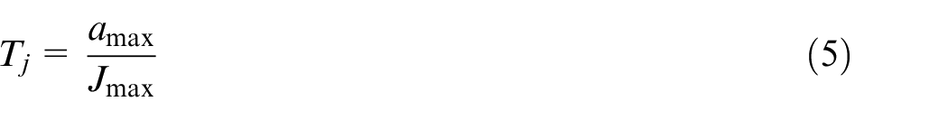
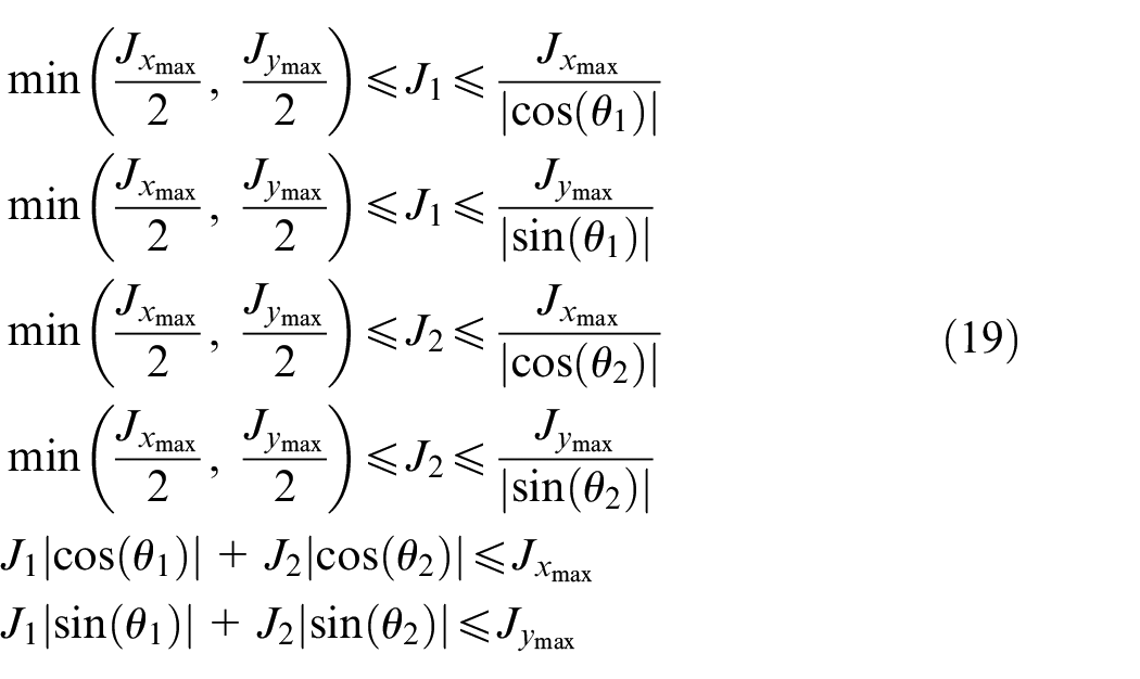
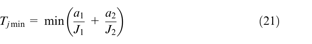
To optimize the machine performance, one optimization index is considered, which is to minimize jerk time as depicted in equation (5). For the problem of minimizing the sum of the jerk time

where
Based on equations (5) and (18), the optimization function can be written as
where
As shown in Figure 9, the feasible search region of
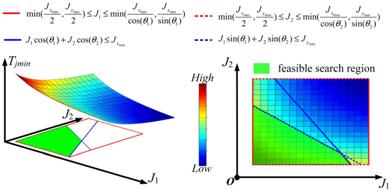
The optimization of jerks.
Simulation and experiment
In this section, the simulations and the experiments are conducted to evaluate the performance of the proposed FBM. Meanwhile, a TCM, which fits cubic B-spline around the corners, 9 is also employed for comparison with the same S-shape feedrate profile. Besides, the parameters used in this section are listed in Table 3.
The parameters used in the experiments.
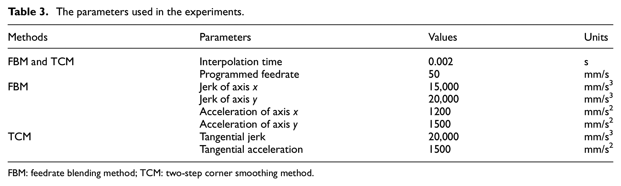
FBM: feedrate blending method; TCM: two-step corner smoothing method.
Simulation
In this section, a simple toolpath with different angles is employed, as depicted in Figure 11. The corner error is set to
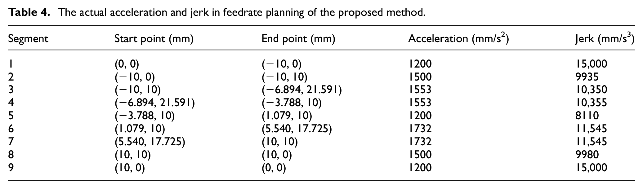
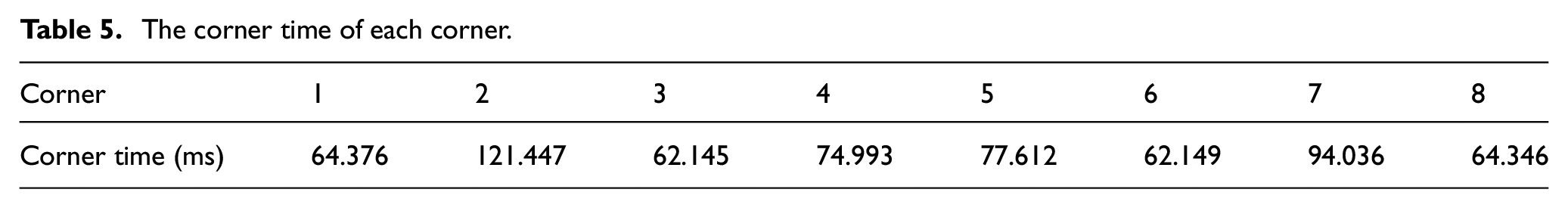
For the proposed FBM, the final acceleration and jerk of each segment used in feedrate scheduling process are listed in Table 4, which can limit the axis jerk and acceleration in the feedrate blending by the algorithms introduced in section “Feedrate blending algorithm for linear segments.” The corner times determined by the corner error are presented in Table 5. It should be noted that there is no need to schedule the feedrate again after the corner time is obtained. When the first segment is decelerating to the start of the corner time, meanwhile the acceleration of second segment will start according to the original scheduled feedrate profiles. Thus, the blending feedrate of the two segments is generated, as depicted in Figure 10.
The actual acceleration and jerk in feedrate planning of the proposed method.
The corner time of each corner.
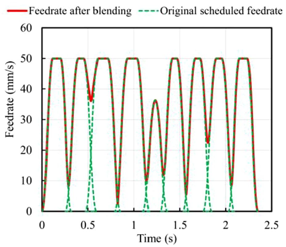
The process of feedrate blending.
For the TCM, the smoothed cubic B-splines at the corners are first generated, and then the centripetal acceleration, the centripetal jerk, and the chord error should be limited in feedrate scheduling process.
9
In this section, the centripetal acceleration, the centripetal jerk, and the chord error are set to
The detailed smoothed trajectories of corners and scheduled feedrate by two algorithms are depicted in Figures 11 and 12, respectively. The maximum corner errors and the minimum feedrate around the corners are presented in Table 6. As presented in Figure 12, the machining time by FBM is 2.350 s, which is reduced by 9.65% compared with TCM. And it can be seen from Figure 11 and Table 6 that the maximum corner errors generated by two methods are controlled within the limitation. In addition, the theoretical corner errors generated by FBM are smaller than those by TCM, which means that the FBM can smooth the tested linear segments with higher efficiency and higher accuracy than TCM.
The maximum corner error and the minimum feedrate of each corner.
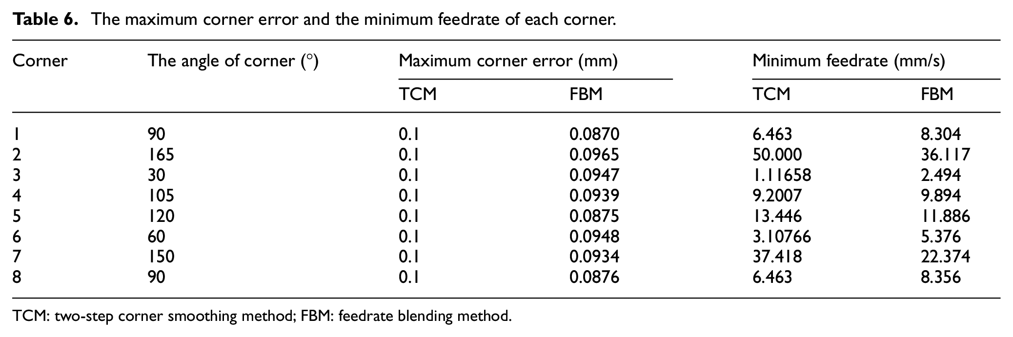
TCM: two-step corner smoothing method; FBM: feedrate blending method.
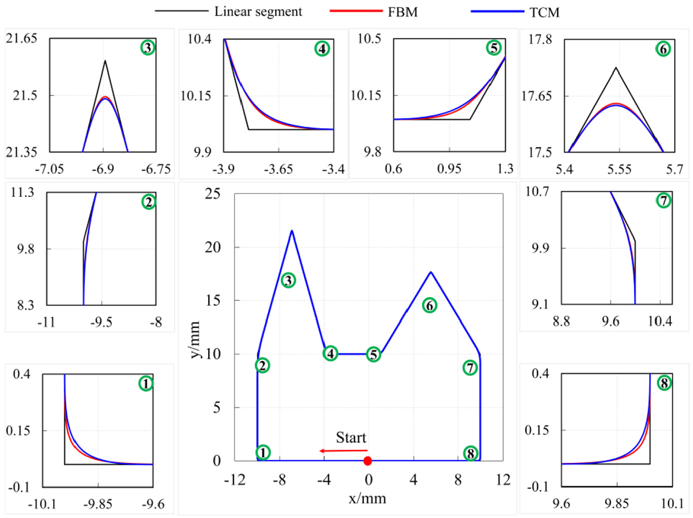
The smoothed toolpath in simulation.
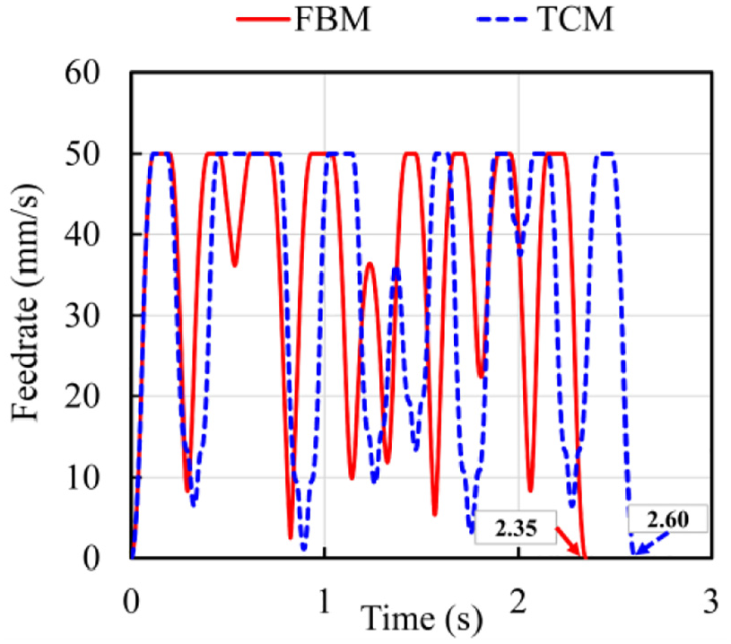
The scheduled feedrate by two algorithms.
Experiment
In order to further evaluate its applicability and performance in the real-time CNC system, two practical toolpaths with obtuse and acute angles together with longer and shorter segments are applied on a three-axis milling CNC machine tool as depicted in Figure 13. The algorithms are carried out on the self-developed CNC system with position feedbacks from motor encoders, and the key processor of which is an ARM 926EJ-STM 400 MHz processor. The cornering tolerance is set to 0.02 mm.
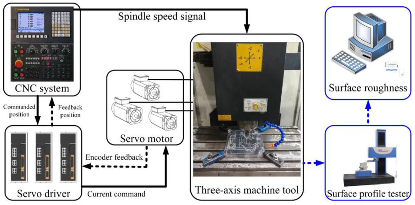
The experimental setup.
First, the leaf-shaped toolpath is tested with the TCM and FBM, as shown in Figure 14. The kinematic profiles by two methods are illustrated in Figures 15 and 16. As depicted in Figure 15, no matter at the longer linear segments or the shorter segments, the feedrate will be blended to smooth the corner within the specified tolerances by two methods. As a consequence, the tool motion will be never stopped to improve machining efficiency. However, the cycle time with FBM is reduced by 8.26% compared with TCM. What’s more, the two algorithms constrain axis feedrate and axis acceleration within the limits, but the axis jerk cannot be limited to the user-specified limits by TCM, as presented in Figure 16, which will affect vibratory and tracking performance of the feed drive system. 25
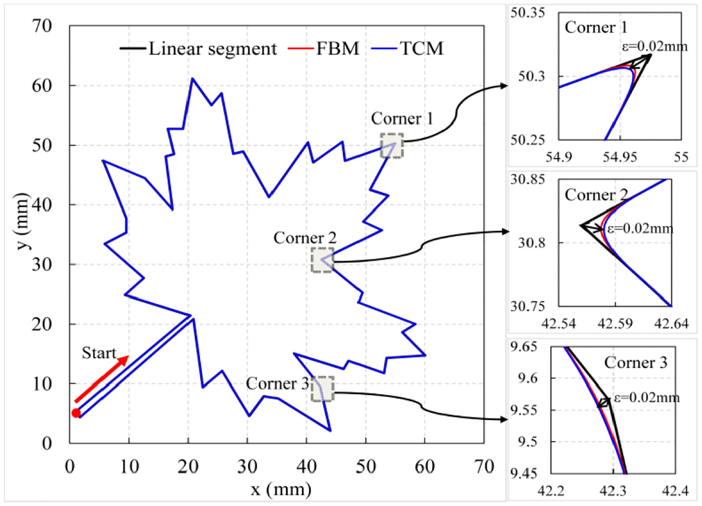
The leaf-shaped toolpath.
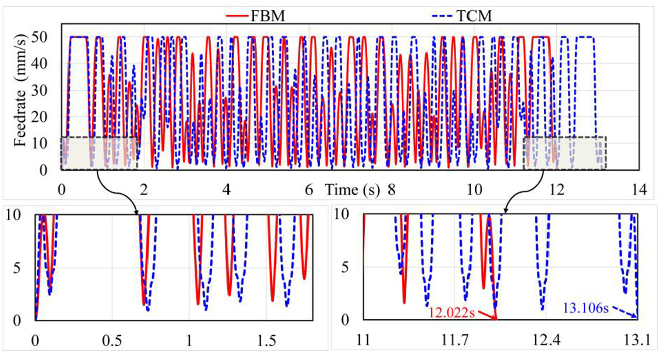
The scheduled feedrate of leaf-shaped toolpath.
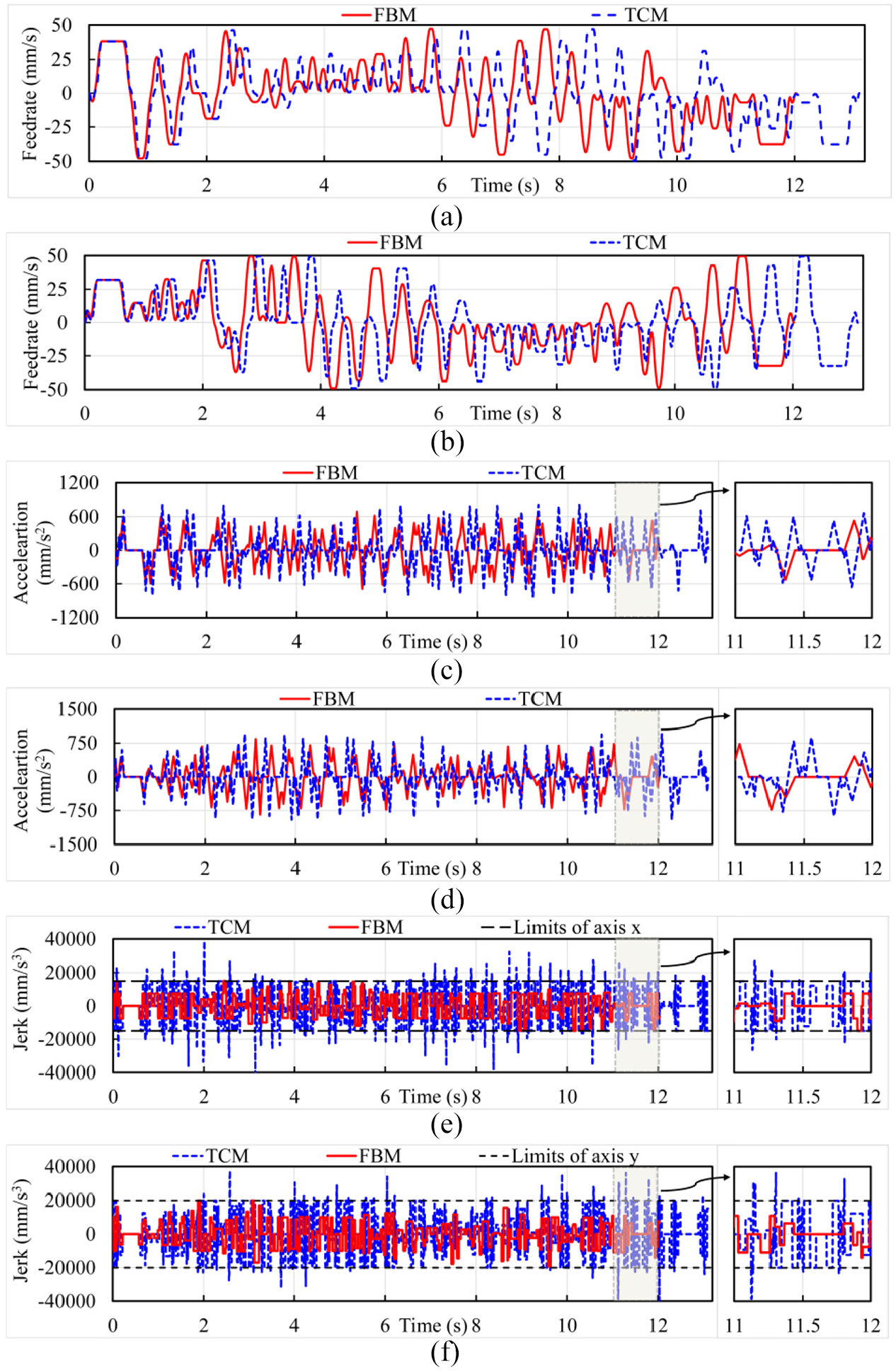
Kinematic profiles by two methods: (a) feedrate of axis x, (b) feedrate of axis y, (c) acceleration of axis x, (d) acceleration of axis y, (e) jerk of axis x, and (f) jerk of axis y.
The estimated contour errors are presented in Figure 17 and summarized in Table 7, in which the performance index “RMS” means the root mean square of contour errors and “Max” means the maximum absolute contour errors. The machining results with 4000 r/min spindle speed on the 6061 aluminum alloy workpiece and the tested areas of the leaf-shaped toolpath are shown in Figure 18. The results of surface roughness at the bottom of the tested areas are shown in Figure 19. It can be seen that the average surface roughness with FBM is slightly better than that with TCM, besides FBM delivers smaller RMS contour error and provides about 13.05% reduction in maximum contour error in the real-time CNC system. As mentioned above, the proposed method can provide a smoother and more accurate trajectory with limited axis dynamic constraints and faster machining time.
The comparison of machining time and contour error of leaf-shaped toolpath.
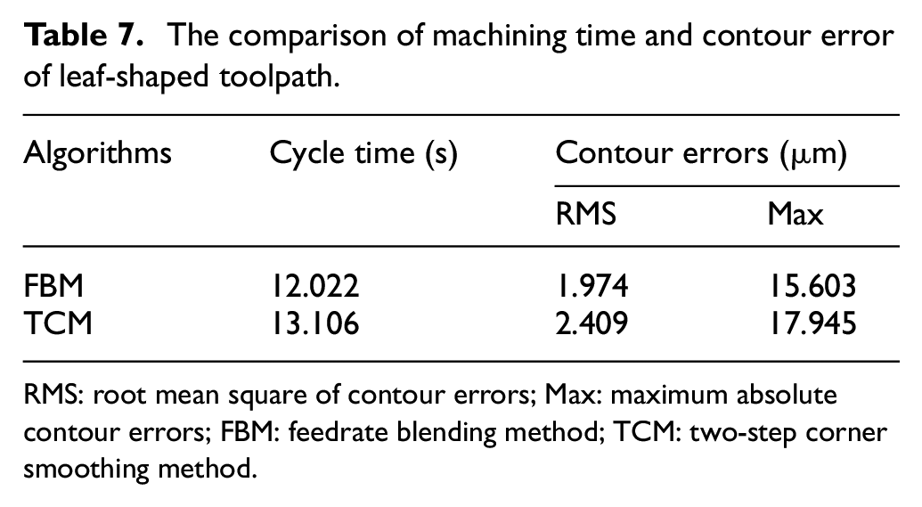
RMS: root mean square of contour errors; Max: maximum absolute contour errors; FBM: feedrate blending method; TCM: two-step corner smoothing method.
The estimated contour errors of leaf-shaped toolpath.
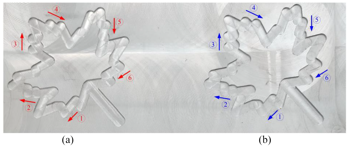
The machining results and the tested areas of the leaf-shaped toolpath: (a) FBM and (b) TCM.
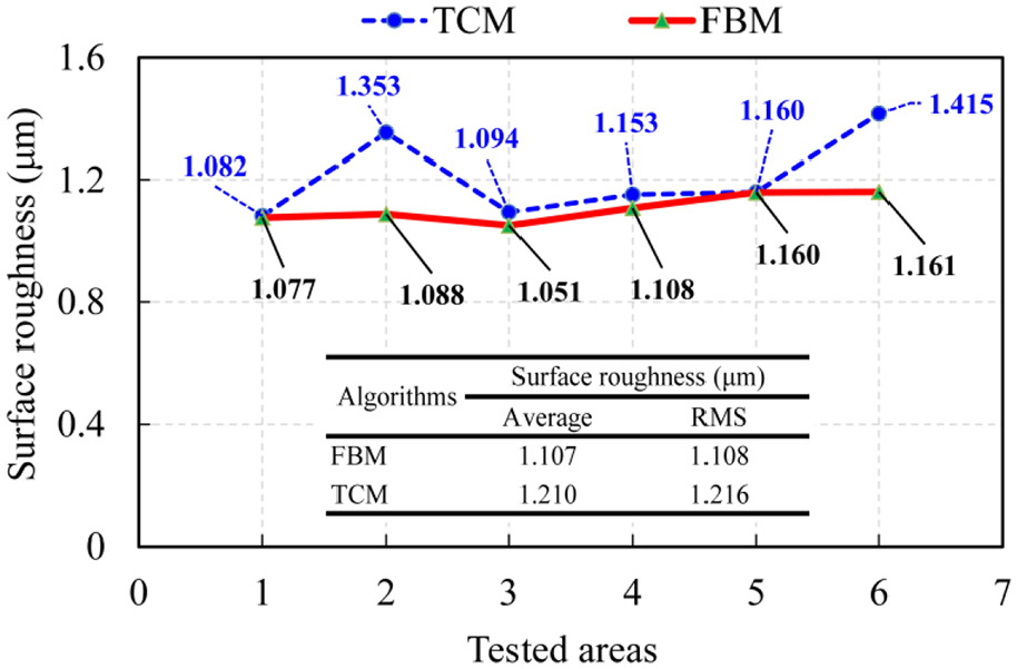
The surface roughness of the tested areas.
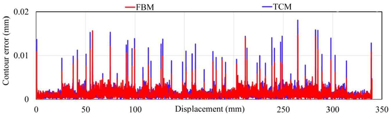
Finally, a more complicated eagle-shaped toolpath with 183 linear segments is performed by TCM and FBM, as observed in Figure 20. The kinematic motion profiles of the two algorithms are depicted in Figures 21 and 22. As shown in Figure 21, the FBM can deliver a faster cycle time than TCM. Observed from the axial jerk profiles in Figure 22(e) and (f), the proposed FBM clearly respects the jerk limits of the drives. However, the axial jerks generated by TCM are out of bounds at most of the corners, which is reflected in contouring performance as shown in Figure 23 and Table 8. As illustrated, the proposed FBM has a better contouring performance with a Max contour error reduction of 3.66% and generates a faster motion with a cycle time reduction of 5.34% compared with the TCM.
The comparison of machining time and contour error of eagle-shaped toolpath.
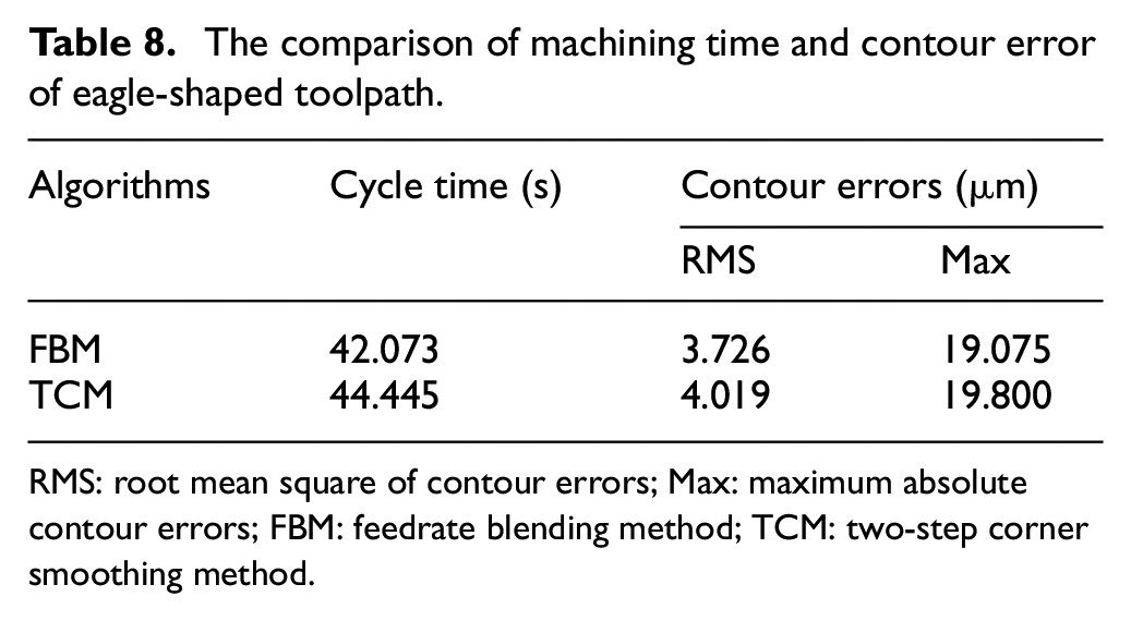
RMS: root mean square of contour errors; Max: maximum absolute contour errors; FBM: feedrate blending method; TCM: two-step corner smoothing method.
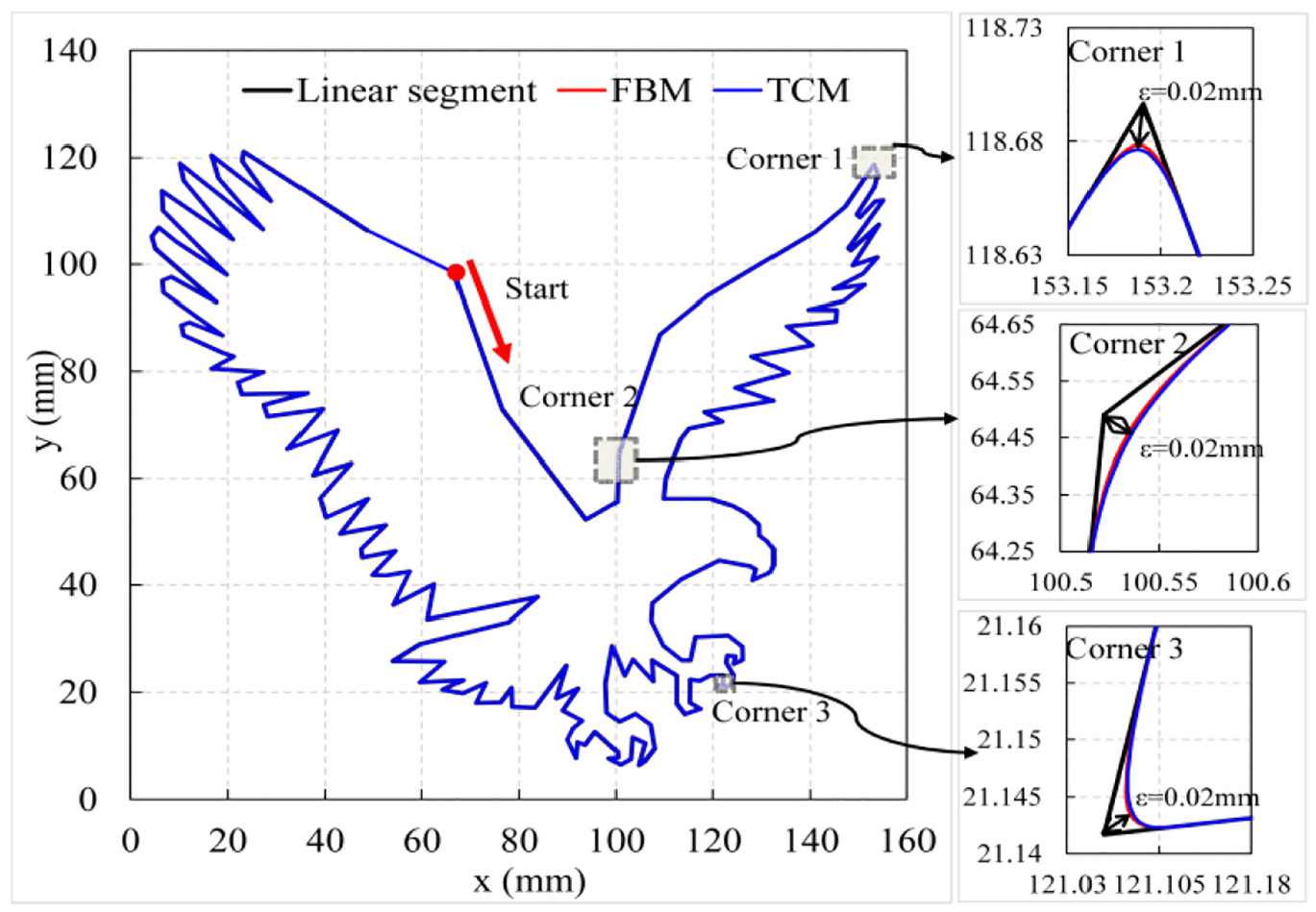
Eagle-shaped toolpath.
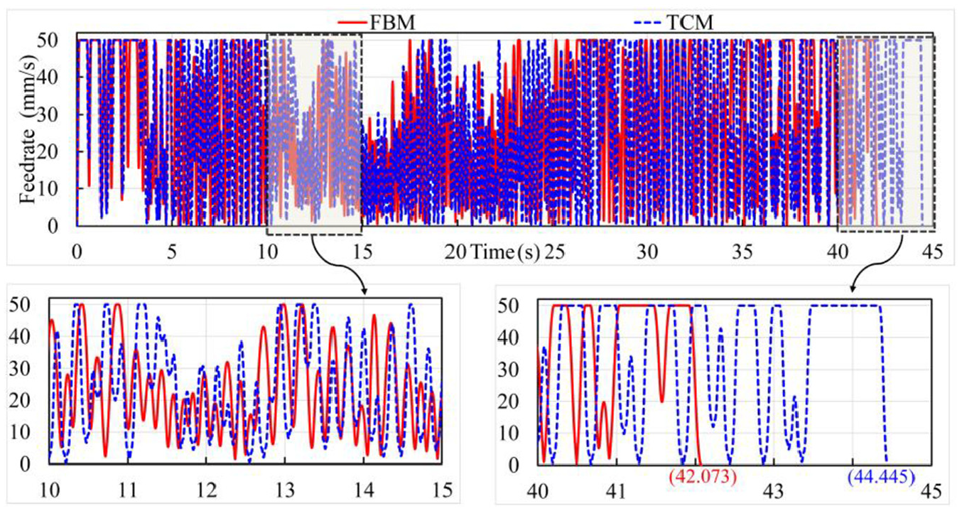
The scheduled feedrate of eagle-shaped toolpath.
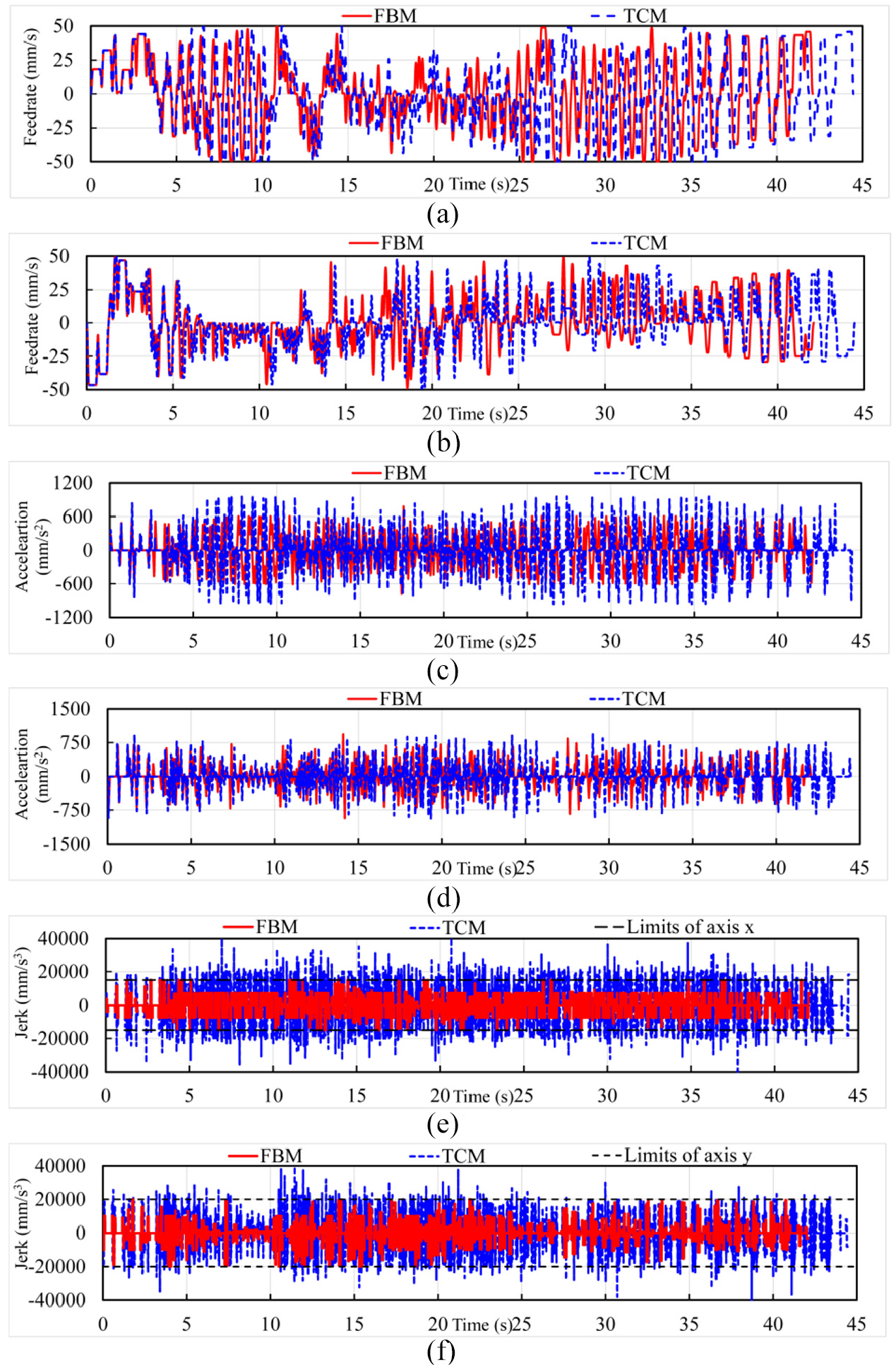
The kinematic profiles of eagle-shaped toolpath: (a) feedrate of axis x, (b) feedrate of axis y, (c) acceleration of axis x, (d) acceleration of axis y, (e) jerk of axis x, and (f) jerk of axis y.
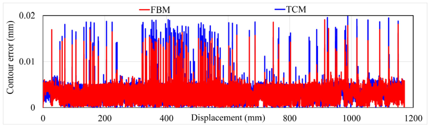
The estimated contour errors of eagle-shaped toolpath.
What’s more, in the blending process, FBM calculates the next interpolation point with an average consuming time of 5.061 μs. Meanwhile, the TCM takes about 277.143 μs to calculate each interpolation point with STE in the real-time ARM-based platform, as illustrated in Figure 24, which will degrade the performance of CNC systems. As a result, the proposed method is computationally efficient and convenient to apply in the real-time CNC system.
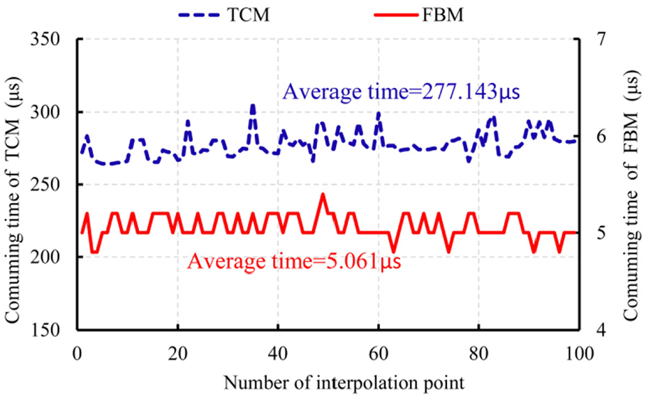
The consuming time to calculate interpolation points.
Conclusion
This article presents a local corner smoothing method with the feedrate blending algorithm, which takes the corner error and axis kinematic constraints into consideration. The proposed method needs only one-step to blend the feedrate and thus to generate the smoothed trajectory around the sharp corner. The corner time can be calculated by the specified corner error, besides the axis acceleration and jerk during the corner time will be limited, since the acceleration and the jerk have been optimized and adjusted in the feedrate scheduling stage. Compared with the TCM with cubic B-spline, the proposed method shows a better contouring performance with faster machining time and has a better real-time performance. Simulations and experiments validate the effectiveness and the feasibility of the proposed method for smoothing linear segments. In future work, the FBM for three-axis and five-axis linear toolpath will be studied.
Footnotes
Appendix 1
Appendix 2
Acknowledgements
The authors express their deepest gratitude to their family for the support.
Author contributions
Y.-B.Z. and T.-Y.W. initiated and developed the ideas related to this research work. Y.-B.Z. derived relevant formulations and carried out the performance analyses of experimental results with the help of Y.-F.L. and R.-J.K. Besides, Y.-B.Z. wrote this article under the guidance of J.-C.D. and T.-Y.W.
Declaration of conflicting interests
The author(s) declared no potential conflicts of interest with respect to the research, authorship, and/or publication of this article.
Funding
The author(s) disclosed receipt of the following financial support for the research, authorship, and/or publication of this article: This work was supported, in part, by the National Natural Science Foundation of China (grant nos 51475324 and 51605328).