
Abstract
Disassembly sequence planning plays a crucial role in the reuse and remanufacturing of end-of-life products. However, it is challenging to obtain optimal disassembly sequences as it is a difficult non-deterministic polynomial-time–hard combinatorial optimisation problem. This study proposes a precedence-based disassembly subset-generation method to solve the disassembly sequence-planning problem. The proposed method first generates disassembly subsets based on disassembly precedence relationships. Subsequently, multiple high-level feasible subsets are generated, and some of them are selected to generate higher level subsets using specially designed operators. After several iterations, different optimal disassembly sequences can be obtained. The principal merit of this method is that high-quality disassembly sequences can be generated in the solution construction process. Numerical experiments were conducted by applying the proposed method to three case studies, and the performance of the proposed method for finding optimal solutions and reducing computational time was evaluated in comparison with state-of-the-art methods. The parameters employed in this method were also analysed to explain the mechanism adopted.
Introduction
Increasing the quantity, updating the technology, and shortening the lifespan of products has resulted in the generation of considerable waste material owing to which the disposal of end-of-life (EOL) products has become a key issue for environmental protection and resource utilisation. 1 Disassembly is one of the most important activities in the recovery and remanufacturing of EOL products. An efficient disassembly process reflects the competitiveness of a company as time is a valuable commodity. In this context, disassembly sequence planning (DSP), which is a major research topic in the disassembly process, determines the order of parts being removed from products. In addition, it has been determined that the DSP problem is a non-deterministic polynomial-time (NP)-hard problem. 2
A large number of reports are available on DSP, and these are mostly focused on (1) developing DSP modelling approaches and (2) developing DSP optimising methods using metaheuristics. 3 Disassembly modelling approaches mainly include the matrix-based method, 4 directed graphs, component-fastener graphs, 5 AND/OR graphs, 6 precedence graphs, cluster graphs, 7 and disassembly Petri net (DPN). 8 Zhang and Zhang, 9 Guo et al., 10 and Song et al. 11 used the cooperative disassembly hierarchical tree generated using a disassembly hybrid graph model (DHGM) to enhance the exploitation capacity of the branch-and-bound algorithm for the cooperative DSP problem. Jiang et al. 12 introduced a product ontology model for generating disassembly tasks for selective disassembly, which takes disassembly tool selection and special connections into consideration. Bahubalendruni and Biswal 13 proposed an assembly model considering four basic predicates, namely, liaison predicate, geometrical feasibility, mechanical feasibility, and stability. Moreover, the influence of assembly predicate has been discussed. 14
To optimise the DSP problem, mathematical programming (MP) has been applied in the past using linear programming, 15 branch-and-bound methods, 16 integer programming, 17 and shortest path algorithms. 18 However, these methods require highly abstract modelling and prior knowledge. Metaheuristic methods have also been adopted to determine cost-effective and feasible disassembly sequences. Song et al. 11 proposed an improved artificial bee colony algorithm to improve the DSP rate of complex products. The feasibility and efficiency of this method were proved by the obtained optimisation results. Guo et al. 10 used a hybrid artificial fish swarm algorithm to solve the DSP problem after considering changes in disassembly directions, tools, and setup time. Tian et al. 19 proposed a novel AND/OR graph–based DSP method after taking changes in the disassembly operational cost and uncertain component quality into consideration. Tseng et al. 20 proposed a new block-based genetic algorithm (block-based GA) for DSP and verified its effectiveness through case studies. Liu et al. 21 used an enhanced discrete bee algorithm for remanufacturing; two gear pumps were used to verify the effectiveness of the proposed algorithm. Yeh 1 proposed a solution for ‘EOL DSP’, using a new soft-computing algorithm that used modified ‘simplified swarm optimisation’. Xia et al.22,23 presented a simplified teaching-learning-based optimisation (TLBO) algorithm to solve DSP problems efficiently. Numerical experiments conducted with case studies demonstrate the effectiveness of the designed operators. Zhang et al. 24 introduced a parallel disassembly sequence-planning method based on fuzzy-rough sets; five disassembly factors were defined and formulated. Two examples were used to validate the proposed algorithm. Ren et al. 25 discussed the selective cooperative disassembly sequence-planning problem in his work. He proposed a new procedure to generate feasible cooperative disassembly sequences and a multi-objective discrete artificial bee colony algorithm to minimise two optimisation objectives. The proposed method was compared with non-dominated sorting genetic algorithm (NSGA-II) to verify its effectiveness. Smith and Hung 26 created a novel selective parallel disassembly planning method for green design. The results of this study showed that the proposed method reduced disassembly costs. Ren et al. 27 proposed an asynchronous parallel disassembly planning, and a GA-based algorithm was modified to solve the DSP problem. Additional intelligent algorithms, such as ant colony optimisation (ACO),28,29 particle swarm optimisation (PSO),18,30 scatter search (SS),31,32 and Tabu search (TS),33,34 have also been applied to address the DSP problem. However, all the methods mentioned above produce disassembly sequences through random generation and their controlling parameters require adjustments, such as the crossover rate and mutation rate in GA and inertia weight and acceleration constant in PSO, which hinders the applicability of these methods in different situations.
An extensive literature survey indicates that little work has been done on using precedence relationships to generate feasible solutions for the DSP problem. In addition, all the cited studies attempted to optimise the disassembly sequence as a whole, which required much time and effort in generating infeasible disassembly sequences; moreover, an optimal disassembly sequence cannot be ensured even after a large number of iterations. Furthermore, the complexity of existing algorithms makes it difficult to reproduce them, which increases the industrial cost of applying these methods. In this study, a precedence-based disassembly subset-generation method integrating a simplified firework algorithm is proposed to find optimal disassembly sequences within a very short period of time. The main contributions of this study are as follows:
Disassembly sequences are generated based on knowledge of precedence graph of the product. Therefore, all the generated sequences are feasible, thus saving considerable computing time by eliminating infeasible disassembly sequences.
This is the first time that the disassembly subset-generation method is applied for DSP. The proposed method generates only one component for each subset and hence the number of iterations required for generating a complete disassembly sequence is equal to the number of components in a product, which overwhelmingly reduces the computing time.
By integrating a simplified firework algorithm with the disassembly subset-generation method, the probability of obtaining an optimal solution becomes higher and different optimal disassembly sequences can be obtained. The main advantage of this method is that it breaks the rule of optimising a disassembly sequence as a whole and finds the optimal solution during the construction process of the disassembly sequence instead of adjusting the order of the complete sequence.
In the proposed method, only two basic size parameters, namely, fireworks size and spark size, are considered. There is no need to tune the controlling parameters, which makes the proposed method adaptive and steady for various situations and easy to reproduce.
The rest of this article is organised as follows. Section ‘Formulation of the disassembly sequence-planning problem’ illustrates the formulation of the disassembly sequence optimisation problem. Section ‘Precedence-based disassembly subset-generation method’ introduces the proposed disassembly subset-generation method using a simplified firework algorithm. Section ‘Case studies and discussion’ presents different disassembly cases, the optimisation results obtained with different methods, and describes the working of the proposed method by analysing key parameters. Finally, Section ‘Conclusion’ summarises the findings of this study.
Formulation of the disassemblysequence-planning problem
Precedence constraints
Precedence constraints are disciplines that take collision-free disassembly capability and part stability into consideration and must be followed when generating a disassembly sequence as they determine its feasibility. There are different ways to represent disassembly precedence constraints, including the precedence graph or matrix, AND/OR graph, 27 and DHGM graph;10,11 different methods are also available for finding the available components. In this investigation, the precedence graph was adopted to analyse different disassembly products.
Figure 1(a) shows a typical example of a two-dimensional (2D) product model. In this model, all the components and joints in the waste product are uniformly considered as components, and there are no differences between components and joints. In this model, joints j1 and j2 are considered as components c4 and c5, respectively. According to the precedence graph shown in Figure 1(b), disassembly precedence relationships can be generated as shown in Table 1. For each row in Table 1, Predecessors have disassembly precedence over Components while Components have disassembly precedence over Successors. For example, c5 should be disassembled before c3, and c3 should be disassembled before c4; ∅ indicates that there are no available components to be disassembled.
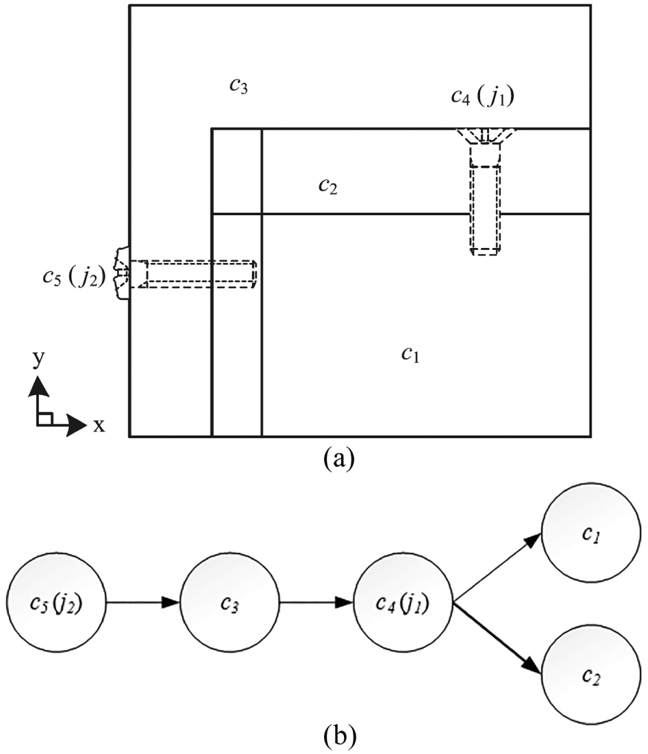
Example of a 2D disassembly product and (b) The precedence graph of the example.
Precedence relationship of the 2D disassembly example in Figure 1.
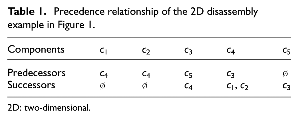
2D: two-dimensional.
Model of disassembly sequence optimisation
In this investigation, all the components and joints in a waste product were considered as components, and the following assumptions were made:
Individual parts were assumed to be rigid solids and contact between them was assumed to be perfect. Disassembly is defined as the removal of all components in a product using non-destructive operations.
Disassembly sequences would be decided in a sequential operation in which one component is removed in each operation.
Each component was characterised by a single removal tool, which was independent of the order of the disassembly sequence.
Apart from the above-listed assumptions, two types of attributes were considered for the disassembly process. They are as follows.
Disassembly direction
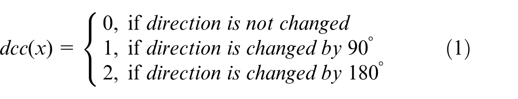
Direction (x) ∈ {± X, ± Y, ± Z}. There are six possible directions and each component must be disassembled in a particular direction. For a change of 90° in the disassembly direction, a cost of 1 is assigned; for a change of 180°, a cost of 2 is assigned; and a cost of 0 is assigned if the disassembly direction is not changed. dcc(x) represents the cost of changing the disassembly direction of component x, and it is calculated as follows
Disassembly tool
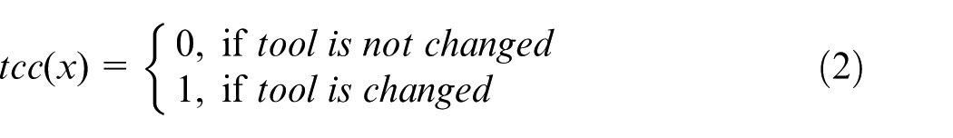
Tool (x) ∈ {T1, …, Tm}, where m is the maximum number of tools used to disassemble a waste product. In disassembly tool, a cost of 1 is assigned if a tool is changed and 0 is assigned otherwise. tcc(x) is the cost of changing the disassembly tool for component x, and it can be calculated as follows
The objective of DSP is to minimise the total disassembly cost while considering the above-described attributes. Let X = (x1, x2, …, xn) be a possible disassembly sequence; then, the objective function is given as follows
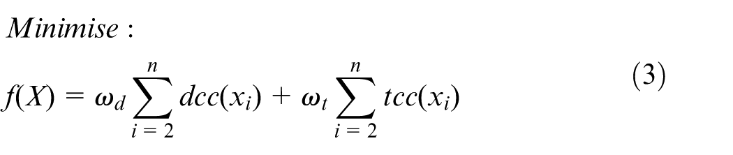
where f(X) represents the total disassembly cost of solution X.
Precedence-based disassembly subset-generation method
Disassembly subset-generation method
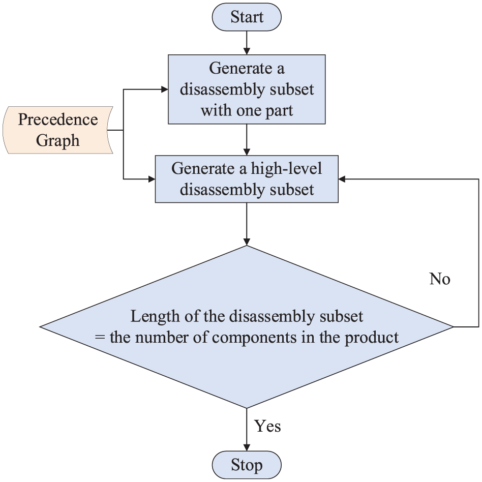
A number of previously reported studies followed the traditional rules of metaheuristics to solve the DSP problem,10,23,27 where the disassembly sequence as a whole is considered and the order of sequence is then adjusted for optimisation. Such procedures require considerable computing time when disassembly products are complex. Inspired by the concept of subassembly detection proposed by Bahubalendruni and Biswal,35,36 which is an efficient method to identify stable subassembly using part concatenation and considering stability relationships between pairs of parts, we propose a novel and simple precedence-based disassembly subset-generation method (DSGM-P) to solve the DSP problem. In this method, only one part is generated for one generation based on knowledge of precedence graph. If the length of disassembly subsets is not equal to the number of components in a disassembly product, a higher level disassembly subset is generated until the condition is met. Thus, the total number of generations required for this method is equal to the number of components in the disassembly product. The basic flowchart of this method is shown in Figure 2, and the pseudo-code of DSGM-P is explained as follows:
Step 1. Input the precedence relationship of a disassembly product
Step 2. Set the predecessors (Pre) and successors (Suc) for each component (C) according to the precedence relationship (precedence graph)
Step 3. Set disassembly sequence (AS) = ∅
Step 4. While length (AS)!= the number of components in the product (P)
Step 5. Available components (AC) = ∅
Step 6. For i = 1 to length (P)
Step 7. If P (i). Pre = ∅
Step 8. Put P (i) into AC
Step 9. End if
Step 10. End for
Step 11. Choose one component from AC randomly
Step 12. Delete this component from the predecessors of all other components
Step 13. Compute its objective function value
Step 14. End while
Step 15. Output a feasible disassembly sequence
Representation of a precedence-based disassembly sequence planning.
DSGM-P using the fireworks algorithm
To obtain optimal disassembly solutions from multiple solutions generated by DSGM-P, a simplified firework algorithm is introduced here. The firework algorithm is a new swarm intelligence algorithm first proposed by Tan and Zhu 37 after observing the natural phenomenon of firework explosions. A batch of sparks, which form the scope of the search space, will be generated around a firework when it explodes. Good-quality sparks continue to explode as a new generation of fireworks. Thus, the firework-explosion process can be regarded as a searching process for the solution space, and the optimal solution in the global space can be obtained by simulating fireworks explosion.
This algorithm mainly consists of three parts – initialisation, explosion, and selection.
Initialisation
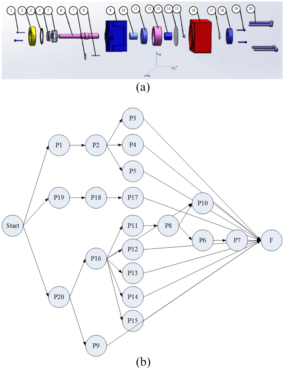
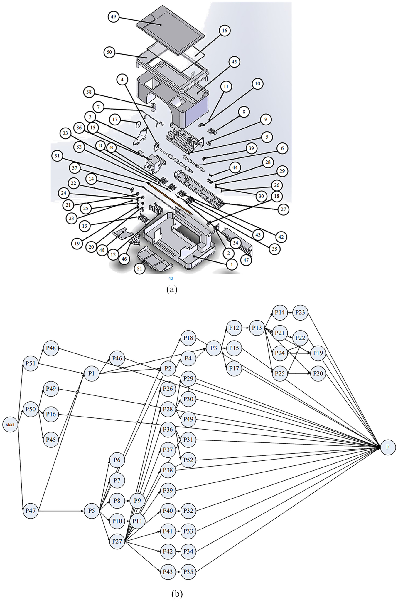
In the initialisation part, N fireworks are generated and initialised by DSGM-P, that is, N disassembly subsets are generated with one component. Taking the product in Figure 6(b) as an example, Components 3, 14, 16, 17, and 18 have no predecessor components and hence can be regarded as the first component. Thus, assuming N = 3, initial disassembly subsets can be written as
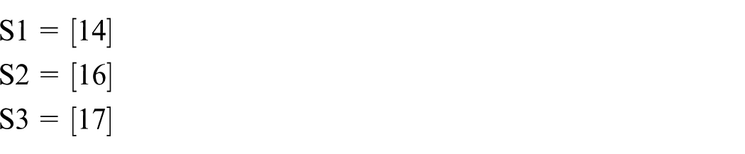
where S represents the disassembly subset sequence.
Explosion
In the explosion part, for each particular firework, a few sparks with higher level subsets are generated to explore the local solution space. All the sparks generated from N fireworks gather together and form a spark pool. Figure 3 shows a simple example of how the explosion operator works. Take the disassembly subset S1 = [14] as an example. After Component 14 is selected in this subset, Component 4 can be removed from the product and it becomes available as the next component. Under these conditions, Components 3, 4, 16, 17, and 18 are available for selection and a component is randomly selected from these five components as the next component. Assuming five sparks are generated from this firework (subset), the next component is selected from the following available sets
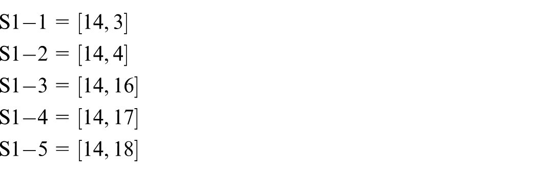
where S1-i represents the ith spark exploding from the first firework.
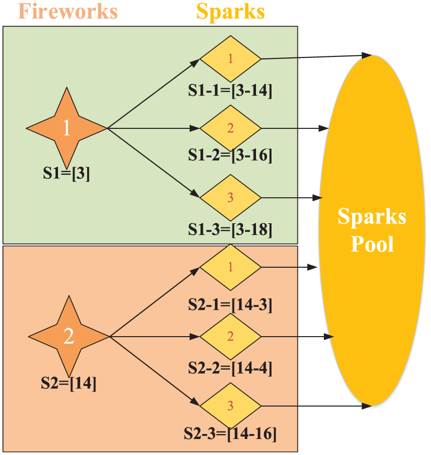
The process of explosion in DSGM-P.
Selection part
The selection part is the most important part of the proposed algorithm. Sparks in the spark pool are ranked according to the objective function of the DSP. Later, N sparks with different disassembly-subset sequences and different objectives are selected as new fireworks for new generations, which are then used to generate higher level disassembly subsets. Unlike traditional methods, which only select solutions with good fitness, in the proposed method, solutions with different fitness and disassembly sequences can be selected even if they represent a poor solution in early stages, which reduces the probability of getting trapped in the local optima. Figure 4 shows the selection process of the proposed algorithm. Assume that there are 12 sparks in the spark pool in total (all sequences and fitness values were generated randomly to illustrate the selection mechanism). Ten new fireworks are to be selected from the spark pool. Eight sparks with different subassembly sequences were selected at first according to their fitness value. Subsequently, the search for the spark resumes from the beginning and new fireworks are selected from the remaining sparks because the number of different sparks is less than the required number of fireworks. Finally, 10 sparks are selected as new fireworks to generate higher level disassembly subsets.
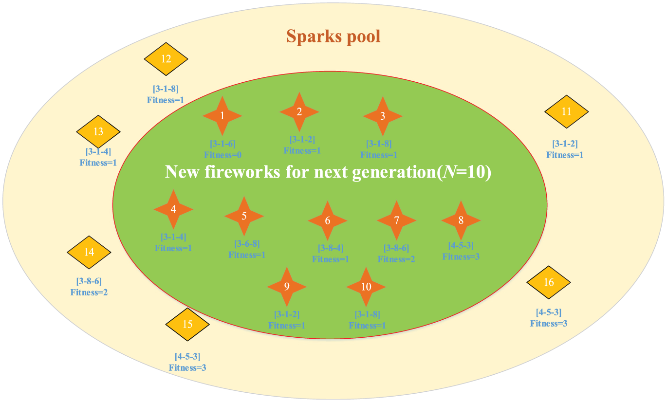
The process of selection in DSGM-P.
The algorithm continues until the total length of disassembly subsets is equal to the number of parts in the disassembly product, and hence, the total number of iterations is equal to the number of components in the disassembly product. This procedure reduces the number of iterations required for obtaining an optimal disassembly sequence by a large extent when compared to other algorithms. The flowchart of the DSGM-P using firework algorithm is shown in Figure 5.
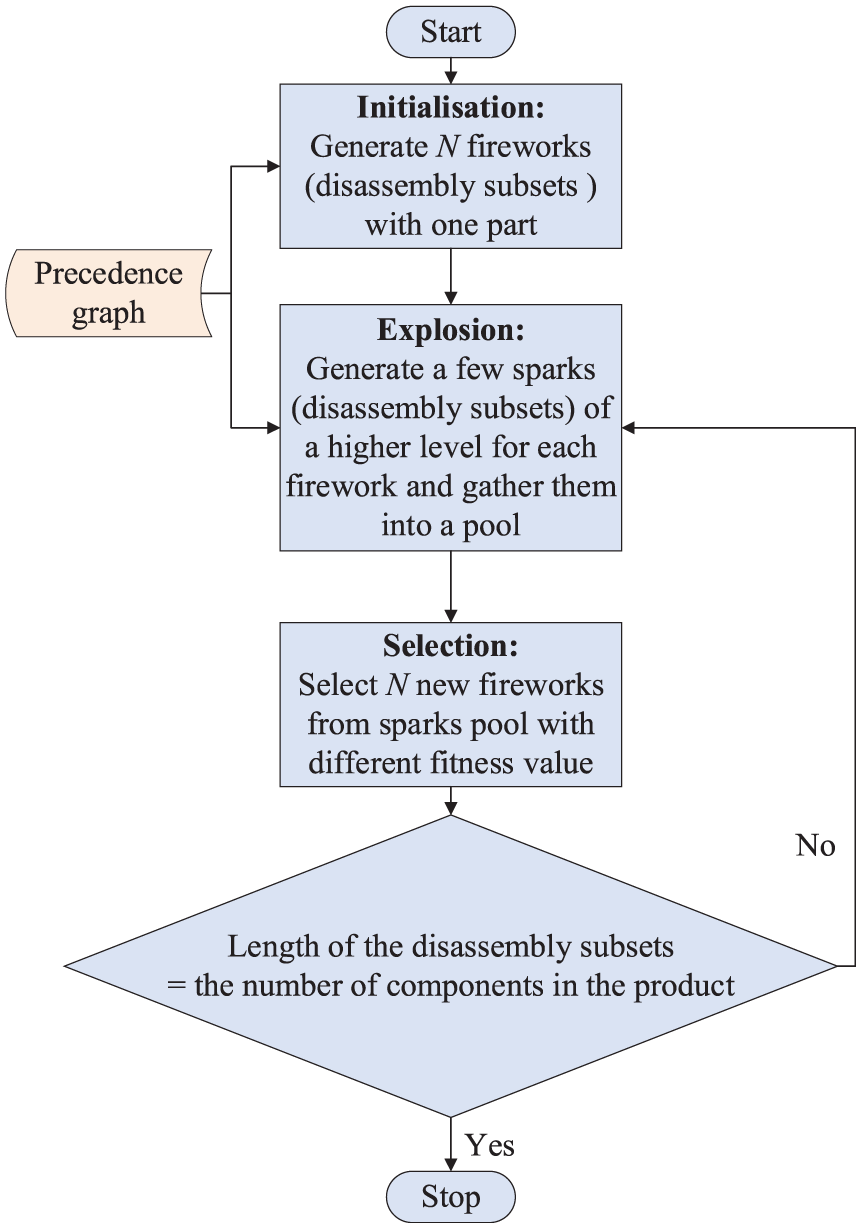
Flowchart of DSGM-P using a simplified firework algorithm.
Case studies and discussion
For numerical experiments and comparison purposes, three disassembly case studies10,20 were used in this study. The performance of the proposed DSGM-P algorithm was evaluated by comparing it with other algorithms, including the GA, ACO, hybrid artificial swarm algorithm (CAAFG), 10 and TLBO.22,23 All the experiments were conducted on MATLAB R2017b on a personal computer with an Intel 2.59 GHz CPU and 8 GB memory. To eliminate pseudo-random effects, 20 runs were conducted for each disassembly case. Based on the obtained values, the optimal fitness and mean fitness were recorded. In addition, the average computing time to complete each algorithm was also calculated.
Stapler
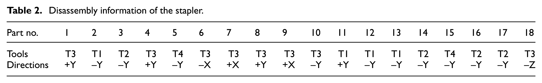
The first disassembly case is a stapler, 20 which consists of 18 components. Figure 6(a) shows the exploding view of the stapler, and Figure 6(b) shows its disassembly precedence graph. Disassembly information, including disassembly direction and disassembly tools for the stapler, is given in Table 2.
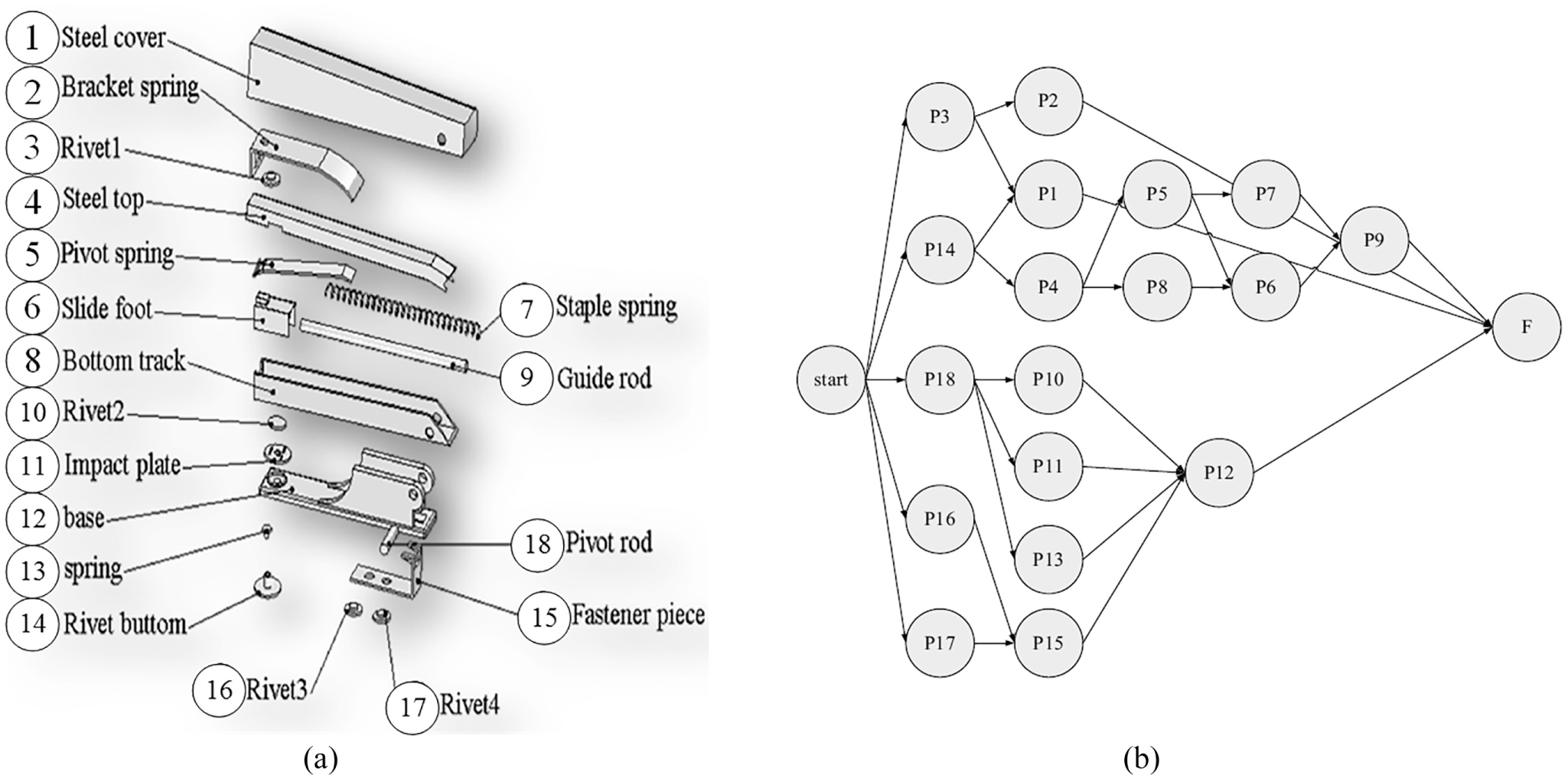
Disassembly information of a stapler: (a) exploded view and (b) disassembly precedence graph.
Disassembly information of the stapler.
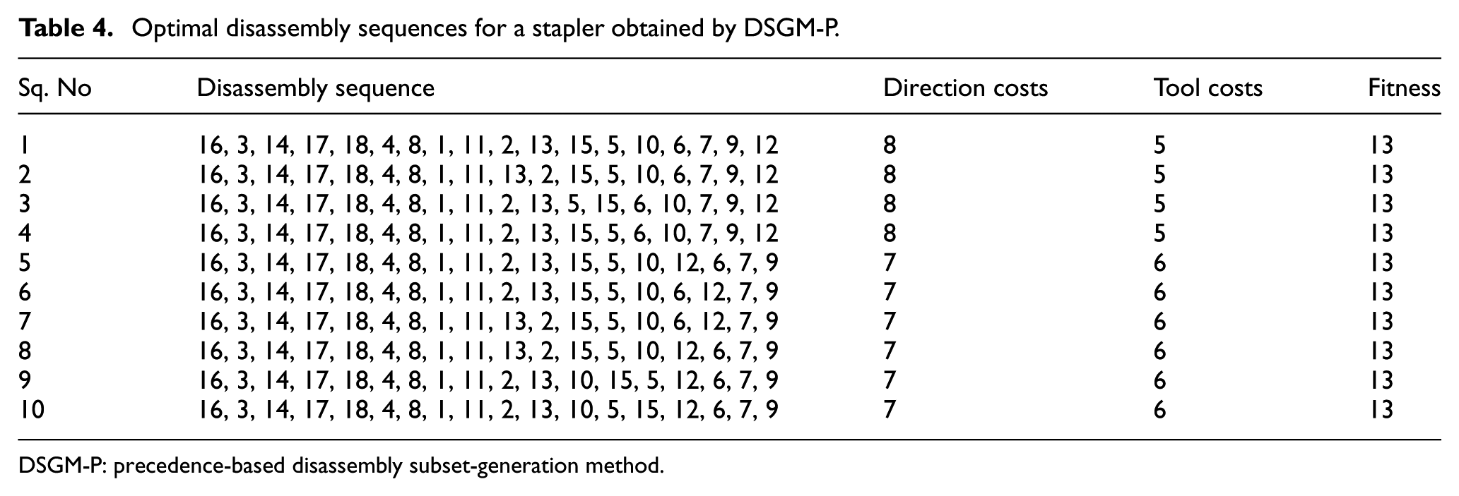
In this case, the population size was set at 30 and the maximum number of generations was 100 for different algorithms. The population size of DSGPM-P was set at 30 and a specific parameter, the number of sparks in DSGM-P, was set at 5. For comparison, the weights of direction changes and tool changes were set as 1, in accordance with the previous article. 20 The optimised results obtained with GA, TLBO, and DSGM-P are shown in Table 3. It can be noticed that although all the algorithms delivered optimal solutions, DSGM-P performs better with respect to average fitness, which shows the robustness of the proposed algorithm. In terms of the average CPU time, DSGM-P required only 1.0595 s while TLBO needed 17.1528 s to finish one run. Hence, it can easily be concluded that DSGM-P is more efficient at obtaining optimal disassembly sequences within a very short period of time. Besides, different optimal solutions are also obtained through DSGM-P, considering the length of the article, and the solutions of 10 optimal disassembly sequences are listed in Table 4.
Optimisation results of the stapler.
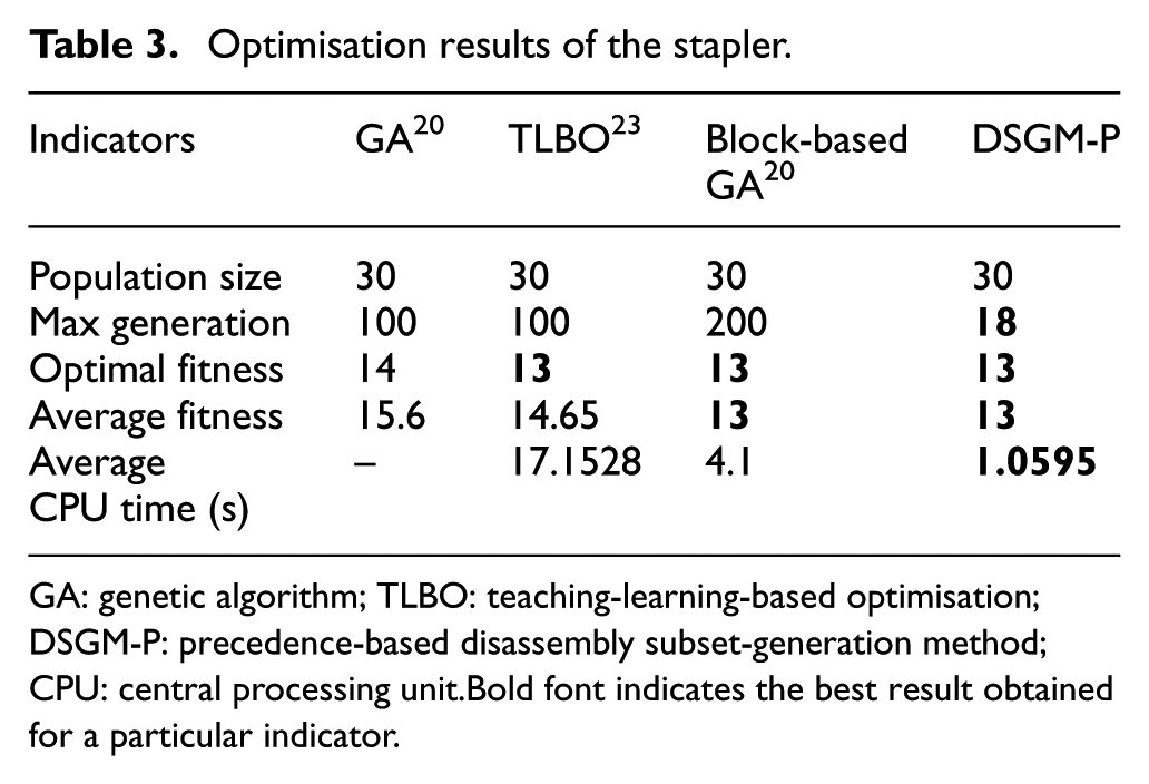
GA: genetic algorithm; TLBO: teaching-learning-based optimisation; DSGM-P: precedence-based disassembly subset-generation method; CPU: central processing unit.Bold font indicates the best result obtained for a particular indicator.
Optimal disassembly sequences for a stapler obtained by DSGM-P.
DSGM-P: precedence-based disassembly subset-generation method.
Internal gear hydraulic pump
The second disassembly case considers an internal gear hydraulic pump,10,11 such as those used in industrial and engineering machinery. Figure 7(a) shows the exploding diagram of the gear hydraulic pump, which has 20 components, and Figure 7(b) shows the corresponding disassembly precedence graph. Disassembly information, including component names, disassembly directions, and disassembly tools, is shown in Table 5.
Disassembly information of a pump: (a) exploded view and (b) disassembly precedence graph.
Disassembly information of the pump.
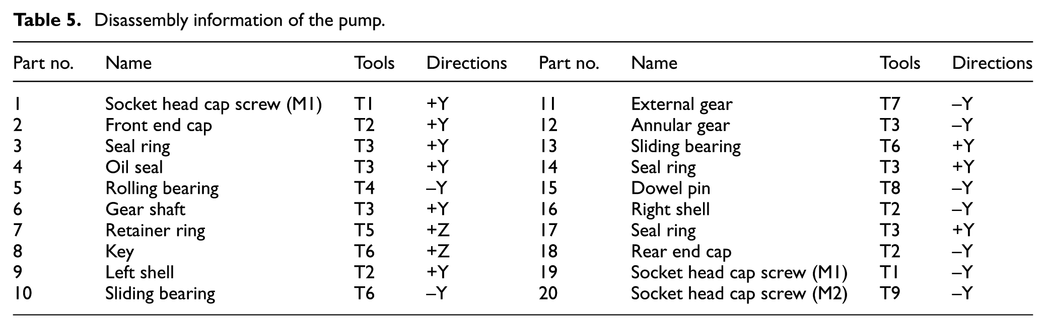
For the pump, the population size was set as 50 and the maximum number of generations was 300 for different algorithms. The number of sparks in DSGM-P was set at 5. For comparison, the weights of direction changes and tool changes were set as 0.25 and 0.75, respectively; this is because in general, tool changes require more time than direction changes in disassembly operations. The optimised results obtained using GA, ACO, CAAFG, 10 TLBO, and DSGM-P are shown in Table 6. It is evident that only DSGM-P could realise an optimal solution in this example. In terms of the average fitness, the performance of DSGM-P is better than that of other algorithms, which shows its superior convergence. As for the average CPU time, DSGM-P required an average of 2.0226 s while TLBO required more than 80 s to finish one run. Considering the complexity of other algorithms, for example, CAAFG, it can easily be concluded that DSGM-P is highly efficient in dealing with the DSP problem. Besides, different optimal solutions are also obtained through DSGM-P, considering the length of the article, and the solution of 10 different optimal disassembly sequences are listed in Table 7.
Optimisation results of the pump.
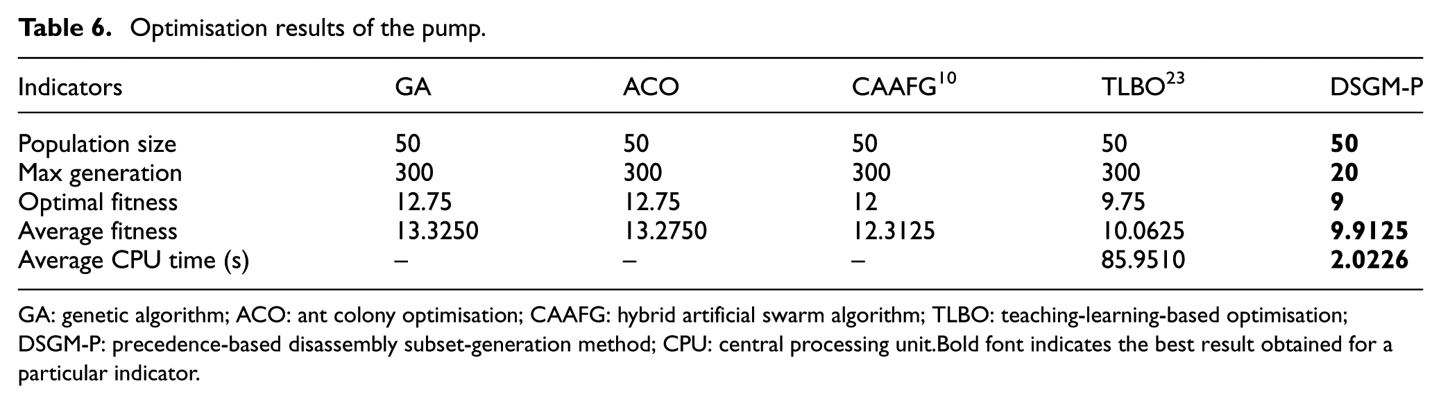
GA: genetic algorithm; ACO: ant colony optimisation; CAAFG: hybrid artificial swarm algorithm; TLBO: teaching-learning-based optimisation; DSGM-P: precedence-based disassembly subset-generation method; CPU: central processing unit.Bold font indicates the best result obtained for a particular indicator.
Optimal disassembly sequences for a pump with 20 components obtained using DSGM-P.
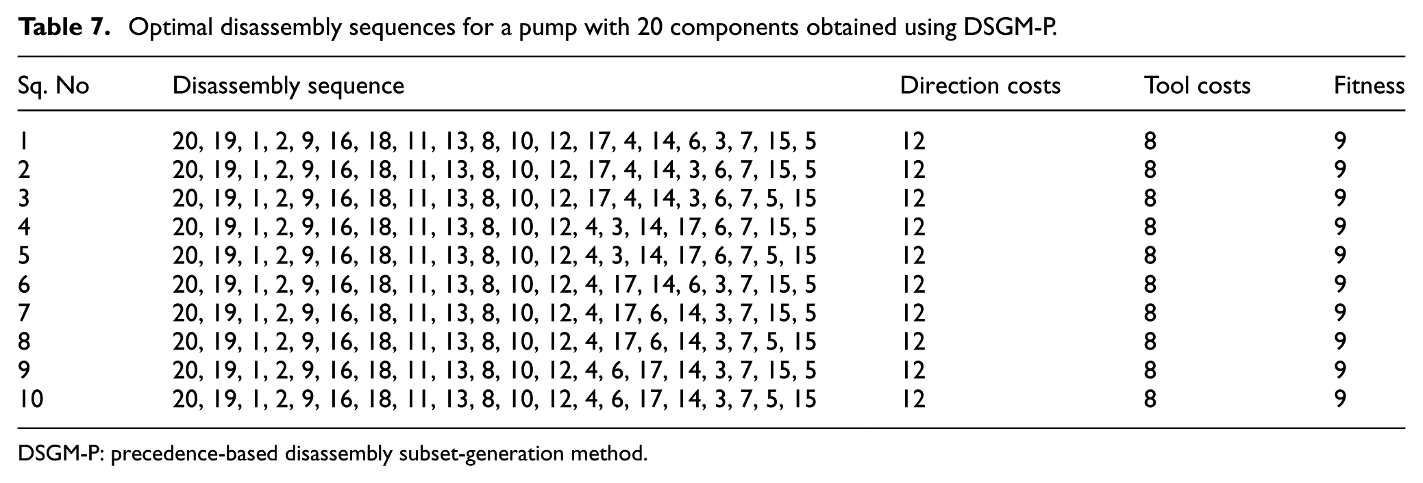
DSGM-P: precedence-based disassembly subset-generation method.
Printer
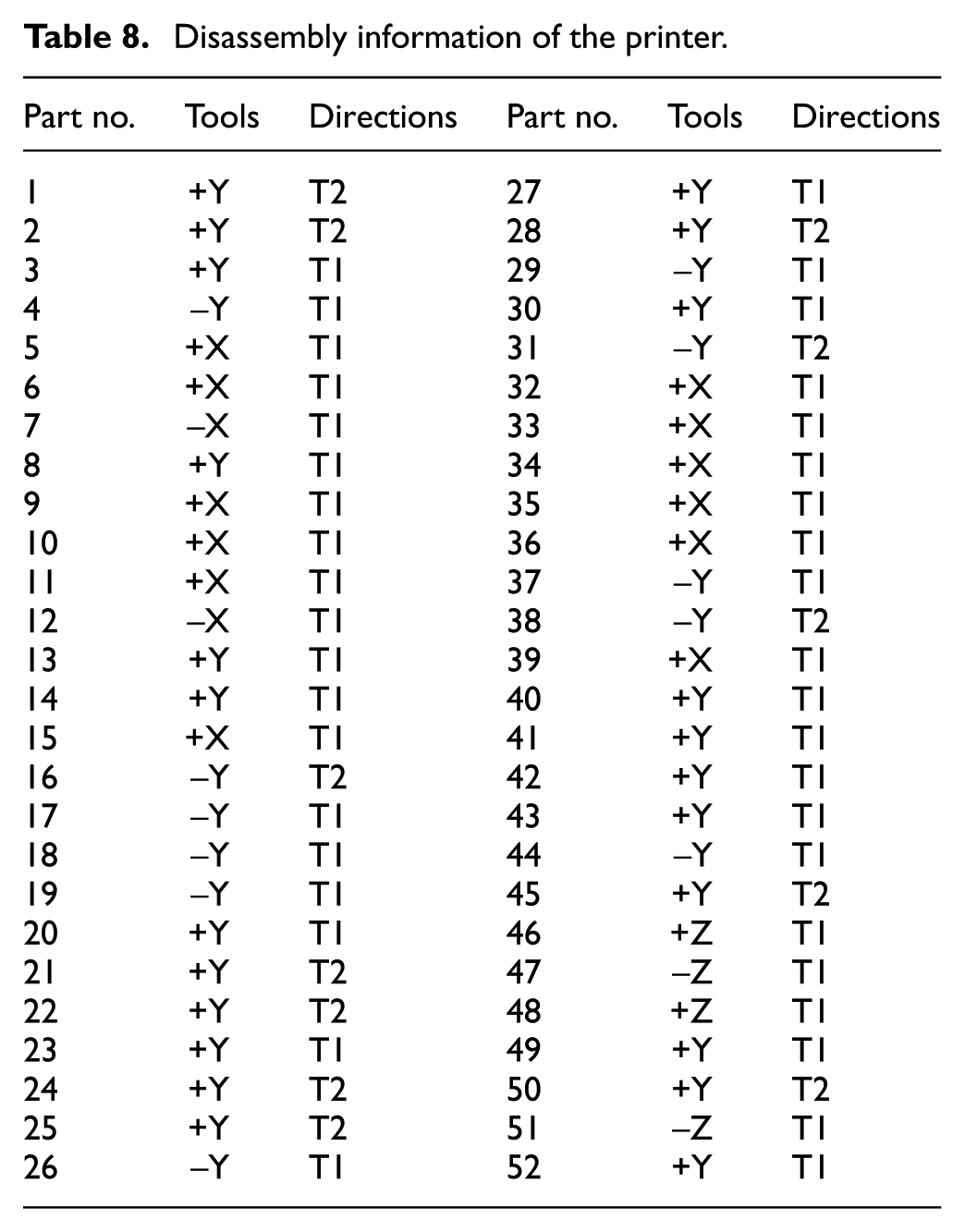
The third disassembly case considered is that of a printer. 20 There are 52 components in the printer. Figure 8(a) shows its exploding view, and Figure 8(b) shows the corresponding disassembly precedence graph. Disassembly information, including component names, disassembly directions, and disassembly tools, is shown in Table 8.
Disassembly information of a printer: (a) exploded view and (b) disassembly precedence graph.
Disassembly information of the printer.
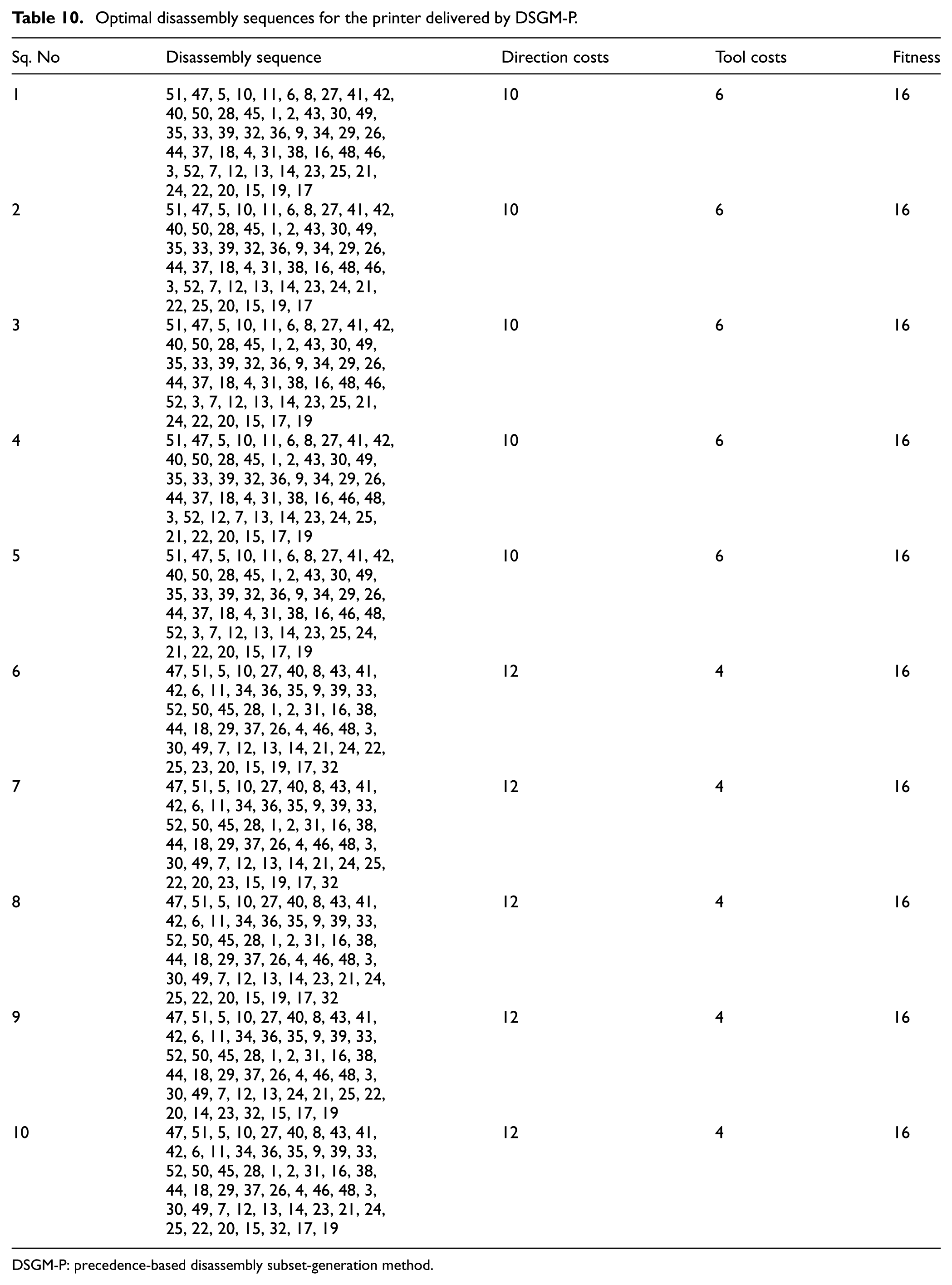
For the printer, the population size was set at 100 and the maximum number of generations was 500 for GA and block-based GA. The maximum number of generations for TLBO was set as 50 because it required very long times on this disassembly product. The number of sparks in DSGM-P was set at 15 for the printer. For comparison, the weights of direction changes and tool changes were set as 1 in accordance with the previous article. 20 The optimised results obtained with GA, TLBO, block-based GA, and DSGM-P are shown in Table 9. It can be inferred from the obtained results that the block-based GA algorithm delivered the best results for this complex product. Although DSGM-P did not yield the most optimal solution, the obtained solutions were still of a high quality with an optimal disassembly cost of 16. Furthermore, DSGM-P performs better than traditional metaheuristic algorithms such as GA and TLBO. As for the average CPU time, DSGM-P required an average of 37.28 s, which is much less than that of the other three algorithms. Ten different optimal solutions obtained by DSGM-P are listed in Table 10.
Optimisation results of the printer.
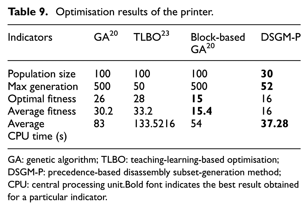
GA: genetic algorithm; TLBO: teaching-learning-based optimisation; DSGM-P: precedence-based disassembly subset-generation method; CPU: central processing unit.Bold font indicates the best result obtained for a particular indicator.
Optimal disassembly sequences for the printer delivered by DSGM-P.
DSGM-P: precedence-based disassembly subset-generation method.
The results of these three different numerical experiments indicate that the proposed DSGM-P algorithm consistently converges to an optimal fitness value within a very short period of CPU time. Therefore, three merits of the DSGM-P method could be verified: (1) all disassembly sequences generated by the DSGM-P method are feasible; (2) the maximum number of iterations required for DSGM-P for disassembly analysis is equal to the number of parts in the device – that is, 18, 20, and 52 for the stapler, the gear hydraulic pump, and the printer, respectively – owing to which computing time can be minimised when disassembling a complicated product; (3) an optimal solution is more likely to be obtained using a simplified firework algorithm. There are two reasons for this observation. One is that the size of the initial population determines the diversity of the solution and DSGM-P can explore the solution space. The other is that the size of sparks generated from each firework controls the exploitation ability of DSGM-P; the more the number of sparks, greater is the local space that can be exploited. The next section presents more detailed experiments and analysis.
Parameter analysis of DSGM-P using the firework algorithm
In this study, a simplified firework algorithm was used to search for optimal solutions. Two parameters were considered in this scenario, the size of fireworks and the size of sparks generated from each firework. The size of fireworks determines the diversity of the solution and DSGM-P explores this solution space. Meanwhile, the size of sparks controls the exploitation ability of DSGM-P; the more the number of sparks, the larger is the local space that can be exploited. To explain this concept more specifically, the disassembly case of the stapler with 18 components is taken as an example.
Figure 9 shows the relationship between initial population size and fitness value of the stapler over 20 runs. The population sizes were 20, 30, 50, 70, and 100. The number of sparks was set as 5 to test the effectiveness of the population size. It can be seen that the optimal fitness value of 13 for stapler disassembly is obtained at all population sizes and the median fitness value gradually decreased with an increase in population size, which means that more solution space was explored. The average CPU time was only 4.14 s even when the population size was 100. In fact, the initial population size determines the diversity of the solution and therefore, more population implies that DSGM-P would have more different disassembly subsets, thus increasing the possibility of obtaining different optimal disassembly sequences.
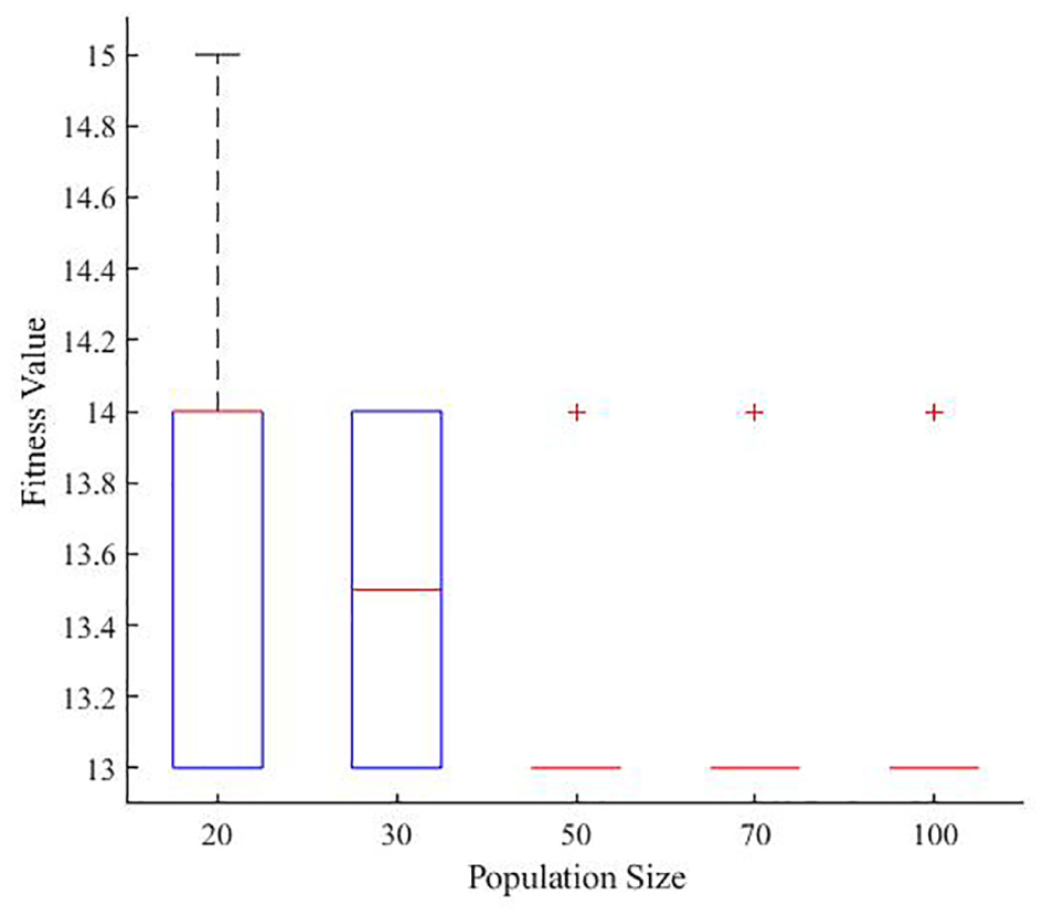
Relationship between population size and fitness value of the stapler.
Figure 10 shows the relationship between spark size and the fitness value of the stapler over 20 runs. The spark sizes were 3, 5, 10, 20, and 50 and the population was set as 30. It can be seen that when the number of sparks was either 3 or 5, the optimal fitness value of 13 was obtained; with an increase in the spark size, the solution tended to be trapped in a local optimum. The main reason is that the number of components in the disassembly product is small. Hence, there are very few independent components without precedence, which means that a small number of sparks is enough to exploit the local space. These results are opposite to those obtained where there are many sparks under the same conditions. The average CPU time was only 9.38 s even when the spark size was 50. In fact, spark size represents the capability of the algorithm to exploit local solution space. With more sparks, the direction of a specific firework can be exploited adequately. However, there is a disadvantage of having too many sparks for a simple disassembly product; furthermore, if there is only a small population, some directions would be exploited too much and many potential solutions would be discarded, leading to a local optimum.
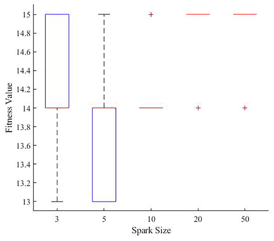
Relationship between spark size and fitness value of the stapler.
Industrial application
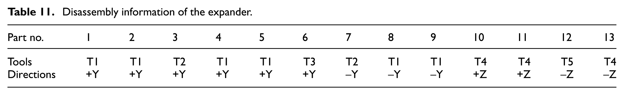
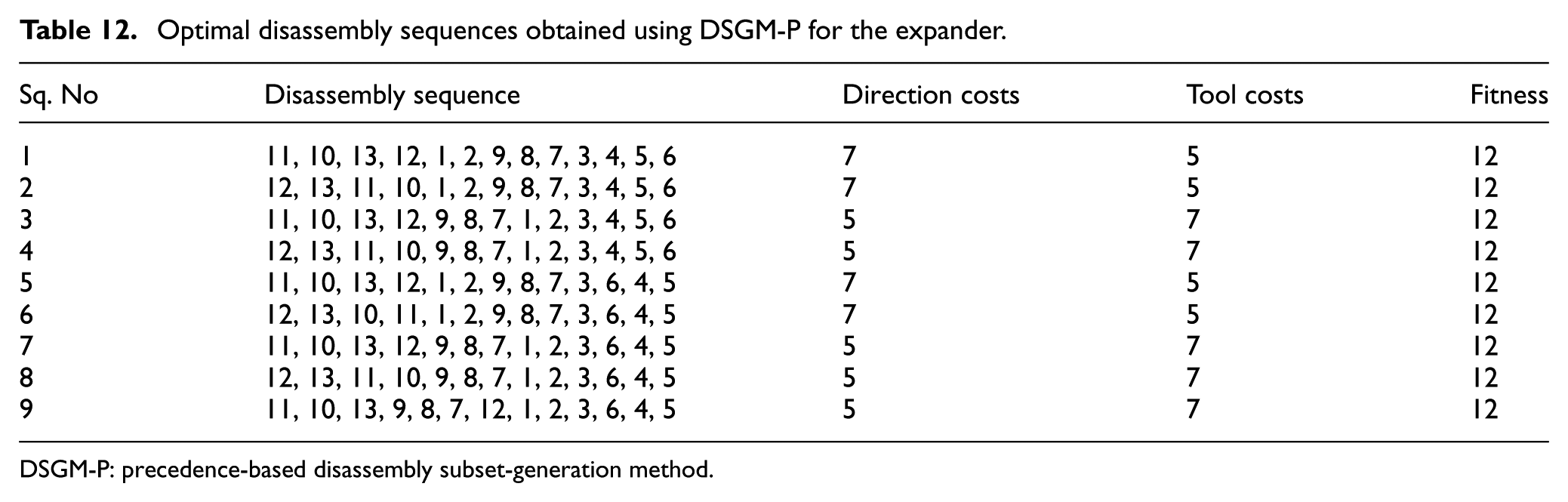
In this section, the proposed algorithm was applied to an industrial product, an expander, which consisted of 13 components. The exploded view of the expander is shown in Figure 11(a), and the disassembly precedence graph is shown in Figure 11(b). The relevant disassembly information is presented in Table 11. Using the proposed algorithm, an optimal objective value of 12 was obtained in only 0.3 s with 20 fireworks and five sparks. A total of nine optimal disassembly sequences were obtained as shown in Table 12.
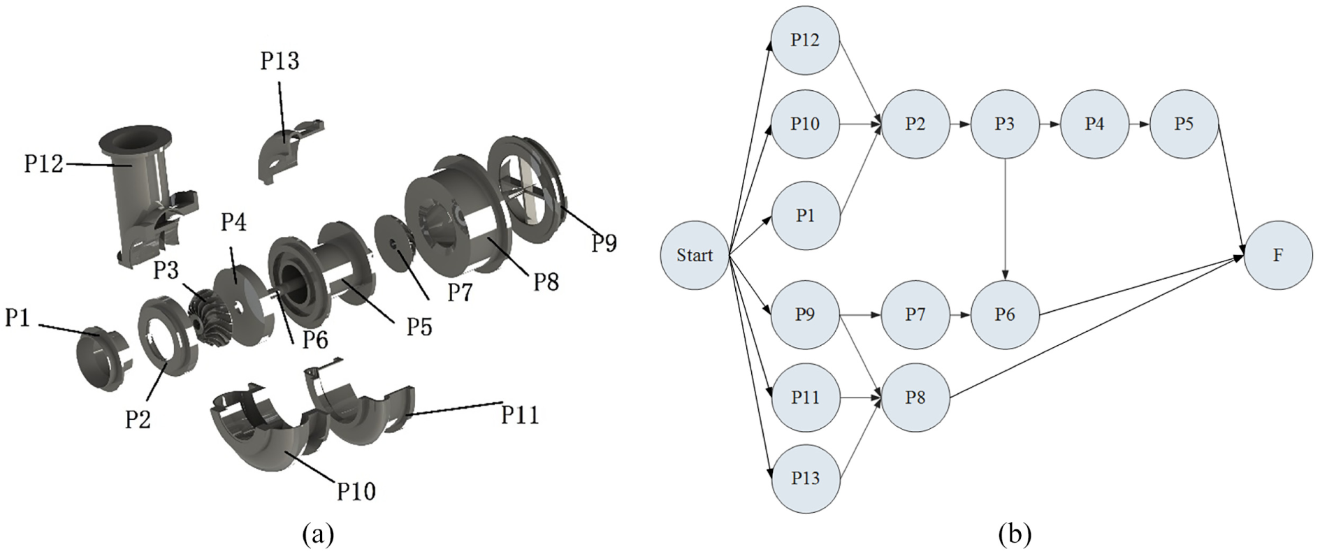
Disassembly information of the expander: (a) exploded view and (b) the corresponding precedence graph.
Disassembly information of the expander.
Optimal disassembly sequences obtained using DSGM-P for the expander.
DSGM-P: precedence-based disassembly subset-generation method.
Conclusion
In this study, we proposed a novel precedence-based disassembly subset-generation method using a simplified firework algorithm to identify disassembly sequences to minimise total disassembly cost. A disassembly precedence graph was adopted to represent precedence constraints between components in a given waste product. Disassembly subsets were generated according to the precedence relationships of the product. A simplified firework algorithm with specially designed operators was introduced to obtain multiple higher level feasible disassembly subsets and select high-quality solutions. The method was tested on three disassembly products with different scales and was compared with several state-of-the-art algorithms. The results show that the proposed method finds the optimal/near-optimal solution within a very short period of time, and its performance is better than that of other algorithms. In addition, two important factors of the proposed method were analysed to understand its working mechanism.
The proposed method has a simple structure and exhibits good performance. It can rapidly provide feasible and effective plans for real-world EOL products and increase the efficiency of the disassembly process, which is crucial for EOL recovery. In future research, parallel operations and more practical attributes, such as the materials in a component and demand after disassembling, will be taken into consideration.
Footnotes
Declaration of conflicting interests
The author(s) declared no potential conflicts of interest with respect to the research, authorship, and/or publication of this article.
Funding
The author(s) disclosed receipt of the following financial support for the research, authorship, and/or publication of this article: This work was supported by the National Natural Science Foundation of China (Grant Nos. 51490663, 51875517, and 51821093), Key Research and Development Programme of Zhejiang Province (Grant No. 2017C01045), and Fundamental Research Funds for the Central Universities (Grant No. 2019FZA4004).