Sage Journals: Discover world-class research

Abstract

Remanufacturing has gained increasing attention due to its economic, environmental and societal benefits as well as its contribution to the sustainability of natural resources. Disassembly is the first and usually the most difficult process in remanufacturing a product. Disassembly sequence planning, which aims to find the optimal disassembly sequence, is required to improve efficiency and reduce cost. There have been many investigations in this field and several disassembly sequence planning methods have been developed. This article reviews the main existing disassembly sequence planning methods from the perspectives of disassembly mode, disassembly modelling and planning method. The characteristics of different methods are analysed and summarised from those perspectives. Future trends in disassembly sequence planning are also discussed to reveal gaps in existing research.

Keywords

Remanufacturing disassembly model optimisation algorithm disassembly sequence planning disassembly sequence optimisation

Introduction

Traditionally, many manufacturing companies have tended to be driven by profits without due regard to energy consumption, pollutant emission and material conservation. This paradigm is no longer viable and modern manufacturing industry must focus on environmental friendliness and sustainable energy and material usage. Remanufacturing provides an economically and environmentally sound way to achieve this by closing the materials use cycle and forming a closed-loop manufacturing system.¹ The essence of remanufacturing is to renew an End-of-Life (EoL) product through appropriate recovery techniques instead of disposing of it through recycling, landfill or incineration.² Landfill and incineration can do harm to the environment, causing air pollution and soil contamination. Recycling of EoL products promotes resource sustainability and can be more environmentally friendly. However, energy consumption could be high for some recycling processes. However, remanufacturing can save energy, production cost and raw materials as well as providing high-value components quickly for production.³ Remanufacturing of an EoL product invariably starts with taking it apart to recover its components. As the condition of the product is not known after years of usage,⁴ traditional disassembly processes have to rely on human operators, which can lead to high costs.

Research efforts have been spent on introducing robots to replace manual labour in disassembly. When dealing with complex disassembly work, humans are more flexible than robots, because machines do not have the knowledge humans use to perform tasks, nor the same capabilities for sensing, perception, reasoning and manipulation. To enable robots to see the product to be disassembled, machine vision has been applied to extract structural information about a product such as its geometrical and locating features.^5–8 To give robots knowledge about how to disassemble a product, researchers have used knowledge bases for storing historical disassembly information and the robots can flexibly deal with their current disassembly tasks using the stored data.^9,10 To optimise the disassembly plan,¹¹ intelligent optimisation algorithms including Particle Swarm Optimisation (PSO),¹² Bees Algorithm,¹³ Artificial Bee Colony (ABC)¹⁴ and Ant Colony Optimisation (ACO)^15–17 can be employed.

A well-designed disassembly sequence helps to improve disassembly efficiency and reduce disassembly cost. The method of finding this well-designed disassembly sequence is called ‘disassembly sequence planning’ (DSP) which is a non-deterministic polynomial (NP) problem.^18,19 DSP^20–23 is to determine the optimal disassembly sequences for given EoL products with considering disassembly precedence relationships. As shown in Figure 1, three steps are involved in DSP, namely, deciding the disassembly mode, building a disassembly model and applying a selected planning method. Of all the steps in DSP, the primary task is to determine suitable disassembly mode for EoL products. After the disassembly mode is determined, disassembly modelling for the EoL product needs to be performed to describe the disassembly precedence relationships between parts or subassemblies. Finally, planning methods should be used to find the optimal solution from various alternatives.

Figure 1.

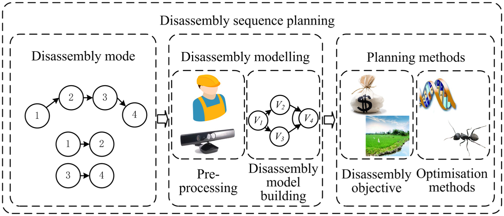
The three steps in DSP.

The disassembly mode should be chosen according to the particular situation (such as complete^24,25 or partial disassembly²⁶). After that, a disassembly model, which describes the disassembly precedence relationship of products,²⁷ should be built to avoid generating unfeasible disassembly sequences. A hybrid disassembly graph was employed to model the contact and non-contact constraints between different parts.²⁶ The Petri net, which includes markings, places, transitions and arcs, is an efficient method to generate feasible disassembly sequences.²⁸ A component-fastener graph was adopted to describe the precedence relationship of EoL products.²⁹ After the disassembly model is built, a suitable planning method is selected to produce the optimal disassembly sequence plan. Planning methods can be differentiated according to the disassembly objective and the optimisation technique used. In terms of disassembly objectives, Shimizu et al.³⁰ combined the time deviation ratio and cost deviation ratio to calculate the fitness function. Kongar and Gupta³¹ proposed fitness functions based on disassembly time, time penalty of method change and time penalty of direction change. Zhang and Zhang³² considered the following factors in calculating fitness: disassembly methods, disassembly types, disassembly directions and corresponding weight. The total disassembly time consisting of standard time, tool changing time and direction changing time was used as the optimisation objective.³³ For optimisation method, intelligent algorithms are the most widely used methods to solve this combinational optimisation problem,^34,35 ACO,²⁶ genetic programming,³⁰ PSO,³² Scatter search (SS)³³ and genetic algorithm (GA)³⁶ have been used to find optimal disassembly sequence.

Although there have been many publications on DSP,³⁷ no recent work can be found that systematically discusses these methods. This article conducts a detailed review of DSP techniques from the perspectives of disassembly mode, disassembly modelling and planning methods. The objective of this review is to discuss the characteristics of the different techniques and identify future research trends.

Disassembly mode

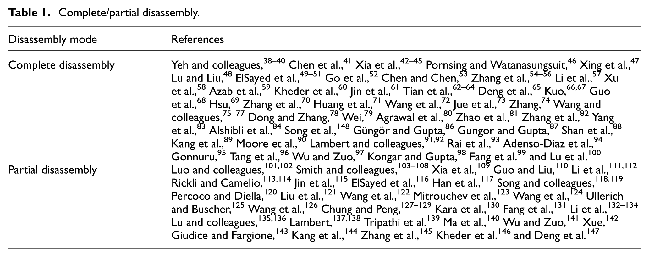
Of all the steps of DSP, choosing a suitable disassembly mode is the first procedure one needs to consider. From the literature reviewed, existing disassembly modes can be grouped in two ways: (1) complete/partial disassembly and (2) sequential/parallel disassembly, as shown in Tables 1 and 2.

Table 1.

Complete/partial disassembly.

Disassembly mode	References
Complete disassembly	Yeh and colleagues,^38–40 Chen et al.,⁴¹ Xia et al.,^42–45 Pornsing and Watanasungsuit,⁴⁶ Xing et al.,⁴⁷ Lu and Liu,⁴⁸ ElSayed et al.,^49–51 Go et al.,⁵² Chen and Chen,⁵³ Zhang et al.,^54–56 Li et al.,⁵⁷ Xu et al.,⁵⁸ Azab et al.,⁵⁹ Kheder et al.,⁶⁰ Jin et al.,⁶¹ Tian et al.,^62–64 Deng et al.,⁶⁵ Kuo,^66,67 Guo et al.,⁶⁸ Hsu,⁶⁹ Zhang et al.,⁷⁰ Huang et al.,⁷¹ Wang et al.,⁷² Jue et al.,⁷³ Zhang,⁷⁴ Wang and colleagues,^75–77 Dong and Zhang,⁷⁸ Wei,⁷⁹ Agrawal et al.,⁸⁰ Zhao et al.,⁸¹ Zhang et al.,⁸² Yang et al.,⁸³ Alshibli et al.,⁸⁴ Song et al.,¹⁴⁸ Güngör and Gupta,⁸⁶ Gungor and Gupta,⁸⁷ Shan et al.,⁸⁸ Kang et al.,⁸⁹ Moore et al.,⁹⁰ Lambert and colleagues,^91,92 Rai et al.,⁹³ Adenso-Diaz et al.,⁹⁴ Gonnuru,⁹⁵ Tang et al.,⁹⁶ Wu and Zuo,⁹⁷ Kongar and Gupta,⁹⁸ Fang et al.⁹⁹ and Lu et al.¹⁰⁰
Partial disassembly	Luo and colleagues,^101,102 Smith and colleagues,^103–108 Xia et al.,¹⁰⁹ Guo and Liu,¹¹⁰ Li et al.,^111,112 Rickli and Camelio,^113,114 Jin et al.,¹¹⁵ ElSayed et al.,¹¹⁶ Han et al.,¹¹⁷ Song and colleagues,^118,119 Percoco and Diella,¹²⁰ Liu et al.,¹²¹ Wang et al.,¹²² Mitrouchev et al.,¹²³ Wang et al.,¹²⁴ Ullerich and Buscher,¹²⁵ Wang et al.,¹²⁶ Chung and Peng,^127–129 Kara et al.,¹³⁰ Fang et al.,¹³¹ Li et al.,^132–134 Lu and colleagues,^135,136 Lambert,^137,138 Tripathi et al.¹³⁹ Ma et al.,¹⁴⁰ Wu and Zuo,¹⁴¹ Xue,¹⁴² Giudice and Fargione,¹⁴³ Kang et al.,¹⁴⁴ Zhang et al.,¹⁴⁵ Kheder et al.¹⁴⁶ and Deng et al.¹⁴⁷

Disassembly mode

References

Complete disassembly

Yeh and colleagues,^38–40 Chen et al.,⁴¹ Xia et al.,^42–45 Pornsing and Watanasungsuit,⁴⁶ Xing et al.,⁴⁷ Lu and Liu,⁴⁸ ElSayed et al.,^49–51 Go et al.,⁵² Chen and Chen,⁵³ Zhang et al.,^54–56 Li et al.,⁵⁷ Xu et al.,⁵⁸ Azab et al.,⁵⁹ Kheder et al.,⁶⁰ Jin et al.,⁶¹ Tian et al.,^62–64 Deng et al.,⁶⁵ Kuo,^66,67 Guo et al.,⁶⁸ Hsu,⁶⁹ Zhang et al.,⁷⁰ Huang et al.,⁷¹ Wang et al.,⁷² Jue et al.,⁷³ Zhang,⁷⁴ Wang and colleagues,^75–77 Dong and Zhang,⁷⁸ Wei,⁷⁹ Agrawal et al.,⁸⁰ Zhao et al.,⁸¹ Zhang et al.,⁸² Yang et al.,⁸³ Alshibli et al.,⁸⁴ Song et al.,¹⁴⁸ Güngör and Gupta,⁸⁶ Gungor and Gupta,⁸⁷ Shan et al.,⁸⁸ Kang et al.,⁸⁹ Moore et al.,⁹⁰ Lambert and colleagues,^91,92 Rai et al.,⁹³ Adenso-Diaz et al.,⁹⁴ Gonnuru,⁹⁵ Tang et al.,⁹⁶ Wu and Zuo,⁹⁷ Kongar and Gupta,⁹⁸ Fang et al.⁹⁹ and Lu et al.¹⁰⁰

Partial disassembly

Luo and colleagues,^101,102 Smith and colleagues,^103–108 Xia et al.,¹⁰⁹ Guo and Liu,¹¹⁰ Li et al.,^111,112 Rickli and Camelio,^113,114 Jin et al.,¹¹⁵ ElSayed et al.,¹¹⁶ Han et al.,¹¹⁷ Song and colleagues,^118,119 Percoco and Diella,¹²⁰ Liu et al.,¹²¹ Wang et al.,¹²² Mitrouchev et al.,¹²³ Wang et al.,¹²⁴ Ullerich and Buscher,¹²⁵ Wang et al.,¹²⁶ Chung and Peng,^127–129 Kara et al.,¹³⁰ Fang et al.,¹³¹ Li et al.,^132–134 Lu and colleagues,^135,136 Lambert,^137,138 Tripathi et al.¹³⁹ Ma et al.,¹⁴⁰ Wu and Zuo,¹⁴¹ Xue,¹⁴² Giudice and Fargione,¹⁴³ Kang et al.,¹⁴⁴ Zhang et al.,¹⁴⁵ Kheder et al.¹⁴⁶ and Deng et al.¹⁴⁷

Table 2.

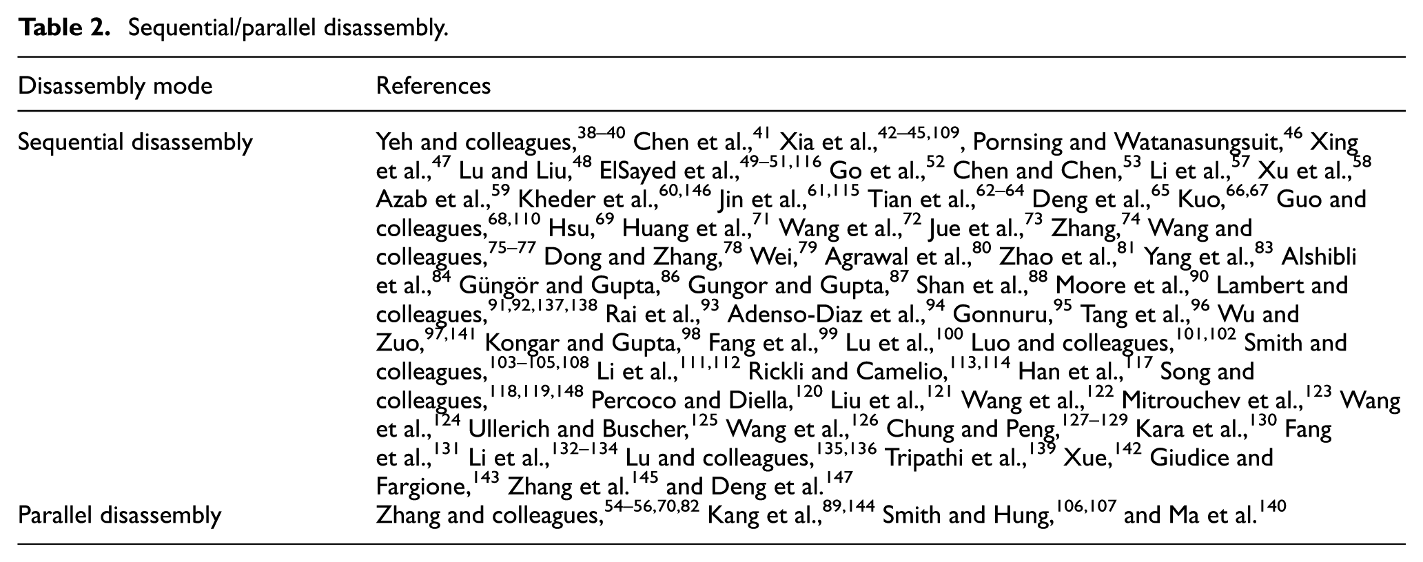
Sequential/parallel disassembly.

Disassembly mode	References
Sequential disassembly	Yeh and colleagues,^38–40 Chen et al.,⁴¹ Xia et al.,^42–45,109, Pornsing and Watanasungsuit,⁴⁶ Xing et al.,⁴⁷ Lu and Liu,⁴⁸ ElSayed et al.,^49–51,116 Go et al.,⁵² Chen and Chen,⁵³ Li et al.,⁵⁷ Xu et al.,⁵⁸ Azab et al.,⁵⁹ Kheder et al.,^60,146 Jin et al.,^61,115 Tian et al.,^62–64 Deng et al.,⁶⁵ Kuo,^66,67 Guo and colleagues,^68,110 Hsu,⁶⁹ Huang et al.,⁷¹ Wang et al.,⁷² Jue et al.,⁷³ Zhang,⁷⁴ Wang and colleagues,^75–77 Dong and Zhang,⁷⁸ Wei,⁷⁹ Agrawal et al.,⁸⁰ Zhao et al.,⁸¹ Yang et al.,⁸³ Alshibli et al.,⁸⁴ Güngör and Gupta,⁸⁶ Gungor and Gupta,⁸⁷ Shan et al.,⁸⁸ Moore et al.,⁹⁰ Lambert and colleagues,^{91,92,137,138} Rai et al.,⁹³ Adenso-Diaz et al.,⁹⁴ Gonnuru,⁹⁵ Tang et al.,⁹⁶ Wu and Zuo,^97,141 Kongar and Gupta,⁹⁸ Fang et al.,⁹⁹ Lu et al.,¹⁰⁰ Luo and colleagues,^101,102 Smith and colleagues,^{103–105,108} Li et al.,^111,112 Rickli and Camelio,^113,114 Han et al.,¹¹⁷ Song and colleagues,^118,119,148 Percoco and Diella,¹²⁰ Liu et al.,¹²¹ Wang et al.,¹²² Mitrouchev et al.,¹²³ Wang et al.,¹²⁴ Ullerich and Buscher,¹²⁵ Wang et al.,¹²⁶ Chung and Peng,^127–129 Kara et al.,¹³⁰ Fang et al.,¹³¹ Li et al.,^132–134 Lu and colleagues,^135,136 Tripathi et al.,¹³⁹ Xue,¹⁴² Giudice and Fargione,¹⁴³ Zhang et al.¹⁴⁵ and Deng et al.¹⁴⁷
Parallel disassembly	Zhang and colleagues,^{54–56,70,82} Kang et al.,^89,144 Smith and Hung,^106,107 and Ma et al.¹⁴⁰

Disassembly mode

References

Sequential disassembly

Yeh and colleagues,^38–40 Chen et al.,⁴¹ Xia et al.,^42–45,109, Pornsing and Watanasungsuit,⁴⁶ Xing et al.,⁴⁷ Lu and Liu,⁴⁸ ElSayed et al.,^49–51,116 Go et al.,⁵² Chen and Chen,⁵³ Li et al.,⁵⁷ Xu et al.,⁵⁸ Azab et al.,⁵⁹ Kheder et al.,^60,146 Jin et al.,^61,115 Tian et al.,^62–64 Deng et al.,⁶⁵ Kuo,^66,67 Guo and colleagues,^68,110 Hsu,⁶⁹ Huang et al.,⁷¹ Wang et al.,⁷² Jue et al.,⁷³ Zhang,⁷⁴ Wang and colleagues,^75–77 Dong and Zhang,⁷⁸ Wei,⁷⁹ Agrawal et al.,⁸⁰ Zhao et al.,⁸¹ Yang et al.,⁸³ Alshibli et al.,⁸⁴ Güngör and Gupta,⁸⁶ Gungor and Gupta,⁸⁷ Shan et al.,⁸⁸ Moore et al.,⁹⁰ Lambert and colleagues,^{91,92,137,138} Rai et al.,⁹³ Adenso-Diaz et al.,⁹⁴ Gonnuru,⁹⁵ Tang et al.,⁹⁶ Wu and Zuo,^97,141 Kongar and Gupta,⁹⁸ Fang et al.,⁹⁹ Lu et al.,¹⁰⁰ Luo and colleagues,^101,102 Smith and colleagues,^{103–105,108} Li et al.,^111,112 Rickli and Camelio,^113,114 Han et al.,¹¹⁷ Song and colleagues,^118,119,148 Percoco and Diella,¹²⁰ Liu et al.,¹²¹ Wang et al.,¹²² Mitrouchev et al.,¹²³ Wang et al.,¹²⁴ Ullerich and Buscher,¹²⁵ Wang et al.,¹²⁶ Chung and Peng,^127–129 Kara et al.,¹³⁰ Fang et al.,¹³¹ Li et al.,^132–134 Lu and colleagues,^135,136 Tripathi et al.,¹³⁹ Xue,¹⁴² Giudice and Fargione,¹⁴³ Zhang et al.¹⁴⁵ and Deng et al.¹⁴⁷

Parallel disassembly

Zhang and colleagues,^{54–56,70,82} Kang et al.,^89,144 Smith and Hung,^106,107 and Ma et al.¹⁴⁰

Complete disassembly involves dismantling an EoL product into individual components, while partial disassembly does not entail the complete breakdown of the product. From Table 1, it is obvious that complete disassembly is the more frequently investigated disassembly mode compared with the partial disassembly mode. Complete disassembly takes longer and costs more, partial disassembly which is to recover high-value components or parts that are difficult to obtain by other means should be considered whenever appropriate.

Table 2 shows references to publications discussing sequential and parallel disassembly. With sequential disassembly, which is the most frequently studied mode, parts are removed from the product one at a time (or in pairs, as in the case of disassembling a nut and a bolt). Parallel disassembly, which involves removing several components simultaneously, can be more efficient. For large complex EoL products, this method should be considered as it can reduce disassembly time compared with the sequential disassembly mode.

Regarding disassembly mode, the numbers of reviewed papers of complete and partial disassembly are, respectively, 63 and 47 and the numbers of reviewed papers of sequential and parallel disassembly are, respectively, 100 and 10. It is apparent that the focus of research so far has been on complete disassembly. However, there are many cases where only partial disassembly is needed, for example, when the aim of disassembly is to retrieve a particular component located in the middle of disassembly sequence for repair, replacement or recycling. Until now, more attention has been paid to sequential disassembly than parallel disassembly. Future work might concentrate on parallel disassembly due to its potential for high efficiency. To date, the only research dealing with both partial and parallel disassembly has been that conducted by Smith and Hung.¹⁰⁷ It is expected that this area will expand in the future when high disassembly efficiency is desired.

Disassembly modelling

After the disassembly mode is determined, disassembly modelling for the EoL product needs to be performed to describe the disassembly precedence relationships between parts or subassemblies. This ensures that unfeasible disassembly sequences are eliminated. Disassembly modelling consists of a pre-processing stage and a model construction stage as shown in Figure 2.

Figure 2.

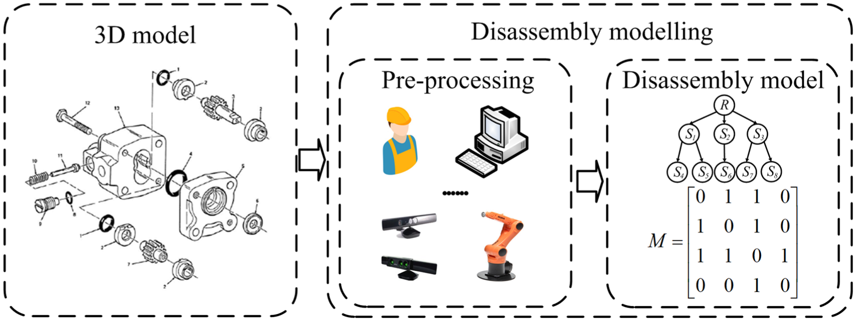
Disassembly modelling process.

Pre-processing

Pre-processing extracts the precedence relationships between different parts from known information about the product such as its computer-aided design (CAD) model. From the literature reviewed, pre-processing tends to be performed manually, as shown in Table 3.

Table 3.

Pre-processing methods.

Methods	References
Manual work	Yeh and colleagues,^38–40 Xia et al.,^42–45,109 Pornsing and Watanasungsuit,⁴⁶ Xing et al.,⁴⁷ Lu and Liu,⁴⁸ ElSayed et al.,^50,116 Go et al.,⁵² Chen and Chen,⁵³ Zhang and colleagues,^54–56 Li et al.,⁵⁷ Xu et al.,⁵⁸ Azab et al.,⁵⁹ Kheder et al.,^60,146 Jin et al.,^61,85,115 Tian et al.,^62–64 Deng et al.,⁶⁵ Kuo,^66,67 Guo and colleagues,^68,110 Hsu,⁶⁹ Huang et al.,⁷¹ Wang et al.,⁷² Jue et al.,⁷³ Zhang,⁷⁴ Wang and colleagues,^75–77 Dong and Zhang,⁷⁸ Wei,⁷⁹ Zhao et al.,⁸¹ Zhang et al.,⁸² Yang et al.,⁸³ Alshibli et al.,⁸⁴ Güngör and Gupta,⁸⁶ Gungor and Gupta,⁸⁷ Shan et al.,⁸⁸ Kang et al.,^89,144 Moore et al.,⁹⁰ Lambert and colleagues,^{91,92,137,138} Rai et al.,⁹³ Adenso-Diaz et al.,⁹⁴ Gonnuru,⁹⁵ Tang and colleagues,^96,149 Wu and Zuo,^97,141 Kongar and Gupta,⁹⁸ Fang et al.,⁹⁹ Lu et al.,¹⁰⁰ Luo and colleagues,^101,102 Smith and colleagues,^103–108 Li et al.,^111,112 Rickli and Camelio,^113,114 Han et al.,¹¹⁷ Song and colleagues,^118,119,148 Percoco and Diella,¹²⁰ Wang et al.,^122,124 Ullerich and Buscher,¹²⁵ Wang et al.,¹²⁶ Chung and Peng,^127–129 Kara et al.,¹³⁰ Fang et al.,¹³¹ Li et al.,^132–134 Lu and colleagues,^135,136 Tripathi et al.,¹³⁹ Ma et al.,¹⁴⁰ Xue,¹⁴² Giudice and Fargione,¹⁴³ Zhang et al.¹⁴⁵ and Deng et al.¹⁴⁷
Visual processing and matching	ElSayed et al.^49,51 and Alshibli et al.⁸⁴
Module of SolidWorks	Agrawal et al.⁸⁰
WFlow	Liu et al.¹²¹

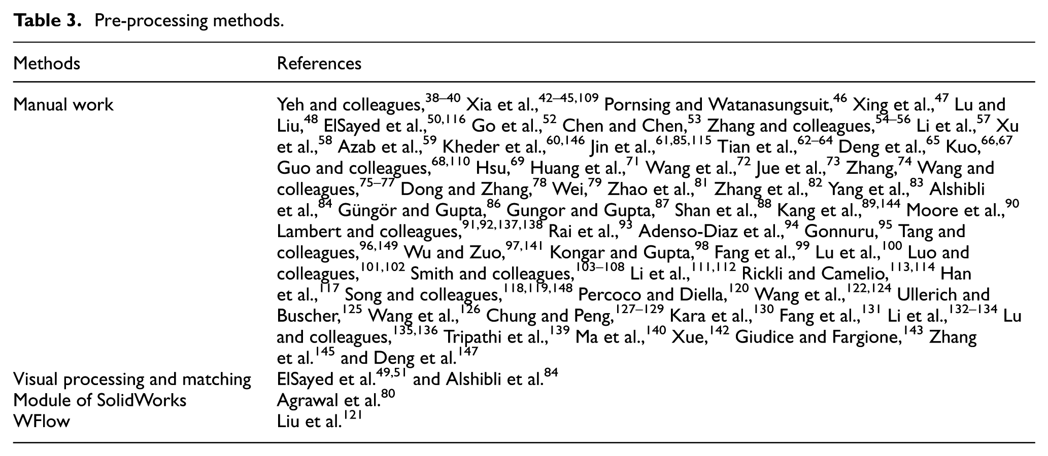
There are 105 papers using manual work to finish pre-processing (NB: if the pre-processing method is not clearly explained in a paper, here, it is taken by default as manually carried out). Due to the powerful recognition and reasoning ability of humans, manual pre-processing is suitable for almost all cases; however, it can be a cumbersome task to extract precedence relationships and generate the disassembly model manually. When the product is complex, manual pre-processing is also an error-prone task which easily leads to the generation of inaccurate models. Thus, automatic pre-processing should be considered to avoid these disadvantages. ElSayed et al.⁴⁹ employed visual processing and pattern recognition for pre-processing. They used visual processing to identify specific components and convolution/correlation-based two-dimensional (2D) template matching to compare the extracted component with the given templates. Their technique was not fully automatic pre-processing because the template had to be provided manually in advance. Apart from the methods just mentioned, Solidworks⁸⁰ and WFlow¹²¹ have also been employed to perform pre-processing, but the details were not clear from these publications.

Regarding pre-processing methods, it is obvious that most of them require manual work. This is because humans are much more flexible and can deal with much more complicated tasks than machines. However, it is time-consuming and error-prone for humans to finish complex tasks when the number of components is large. In addition, most pre-processing methods can be finished only if CAD models are provided. However, after years of usage, EoL products can rarely be described accurately by the original CAD model. Thus, manual work is necessary to adjust existing CAD models or create new representations of actual components. Some researchers have tried to use visual information to exact the precedence relationships between different parts,^8,9 but that simply is not enough. For example, contact forces between different components during disassembly could also yield useful information on the condition of the process which helps to build accurate disassembly models. However, no research has been conducted on this.

Disassembly model building

Disassembly model building is used to produce a model representing the disassembly precedence relationships through specific methods like graphs and matrices. Table 4 shows that disassembly models can be divided into four categories: graphs, Petri nets, matrix-based and other model types.

Table 4.

Disassembly model building methods.

Methods	Description	References
Graph-based method
Disassembly tree	The tree starts from the root node which indicates the original EoL product; the branch nodes represent subassemblies or parts of the product.	Yeh and colleagues,^38–40 Xia et al.,^42,45 ElSayed et al.,^49–51,116 Go et al.,⁵² Azab et al.,⁵⁹ Kuo,⁶⁷ Wang and colleagues,^76,77 Alshibli et al.,⁸⁴ Lambert and colleagues,^{91,92,137,138} Gonnuru,⁹⁵ Kongar and Gupta,⁹⁸ Guo and Liu,¹¹⁰ Han et al.,¹¹⁷ Lu et al.,¹³⁵ Tripathi et al.,¹³⁹ Ma et al.¹⁴⁰ and Xue¹⁴²
Disassembly network graph	Three-element graph: This includes the minimal disassembled part, directed edges and the relationship between pairs of parts.	Chen and Chen,⁵³ Tian et al.,^63,64 Wang et al.,⁷² Wu and Zuo,⁹⁷ Fang et al.,¹³¹ Li et al.^132–134 and Deng et al.¹⁴⁷
	Four-element graph: This includes the minimal disassembled part, undirected/directed edges and directed dotted edges.	Zhang and colleagues,^54–56 Zhang et al.⁸² and Wu and Zuo¹⁴¹
	Five-element graph: This includes the minimal disassembled part, one undirected edge and three directed edges which indicate different constraint relationships.	Song and colleagues^118,119,148
State representation–based disassembly graph	This describes the structure of the EoL product at several disassembly levels.	Tian et al.,⁶² Jue et al.,⁷³ Wei,⁷⁹ Wang et al.,¹²² Mitrouchev et al.¹²³ and Kara et al.¹³⁰
Directed flow disassembly network	This graph-based method starts from one node and ends in another node.	Huang et al.,⁷¹ Kang et al.^89,144 Rickli and Camelio,^113,114 Liu et al.,¹²¹ and Ullerich and Buscher¹²⁵
Petri net method
Simplified disassembly Petri net	This includes the number of places and transitions, places, transitions, place-transition matrix and transition-place matrix.	Rai et al.,⁹³ Xia et al.¹⁰⁹ and Zhang et al.¹⁴⁵
Extended disassembly Petri net	This Petri net includes only one non-leaf output place exists in each transition.	Tang and Zhou¹⁴⁹
Extended stochastic disassembly Petri net	This is a high-level Petri net with arbitrary distribution.	Deng et al.⁶⁵
Disassembly tree Petri net	This comprises four steps: identification, determination of the disassembly rate, construction and evaluation.	Kuo⁶⁶
Disassembly Petri net	This includes an eight-tuple: places, transitions, input and output functions, marking, disassembly cost, recycling value and weight function.	Guo et al.⁶⁸ and Moore et al.⁹⁰
Fuzzy attributed Petri net	Fuzzy sets theory is combined with Petri net to handle the uncertainties in the disassembly process.	Hsu⁶⁹ and Tang et al.⁹⁶
Synchronous net	This employs reduction principles which include S-Combination, T-Combination and place combination.	Dong and Zhang⁷⁸
Fuzzy reasoning Petri net	This is derived from the basic Petri net and its objective is knowledge representation and logic reasoning.	Zhao et al.⁸¹
Matrix-based method
Disassembly interference matrix	Simple case: the element a_ij is set to non-zero if disassembly operation i precedes operation j, and 0 otherwise.	Zhang⁷⁴ and Yang et al.⁸³
	Six-direction matrix: This describes the relative position (±x, ±y, ±z) between different components.	Xia et al.,^43,44 Xing et al.,⁴⁷ Xu et al.,⁵⁸ Jin et al.,^61,85,115 Wei,⁷⁹ Agrawal et al.,⁸⁰ Güngör and Gupta,⁸⁶ Gungor and Gupta,⁸⁷ Shan et al.,⁸⁸ Adenso-Diaz et al.,⁹⁴ Fang et al.,⁹⁹ Lu et al.,¹⁰⁰ Percoco and Diella,¹²⁰ Wang et al.,¹²⁶ Lu and colleagues,^135,136 Giudice and Fargione¹⁴³ and Kheder et al.¹⁴⁶
	Multi-direction matrix: This includes the global precedence matrix and local precedence matrix.	Li et al.⁵⁷ and Luo and Peng¹⁰²
Multi-layer representation method	This method includes several levels and the corresponding representation matrix to reduce storage space and search time, compared with the traditional matrix representation method.	Wang,⁷⁵ Luo et al.¹⁰¹ and Wang et al.¹²⁴
Disassembly sequence structure method	Four-matrix method: This includes disassembly matrices for fasteners and components and motion constraint matrices for fasteners and components	Smith and colleagues^103,107,108
Disassembly sequence structure method	Five-matrix method: Besides the description matrices used in the four-matrix method, there is also a projection matrix for components.	Smith and colleagues^104–106
Dynamic disassembly precedence matrix	The precedence matrix is generated iteratively according to the dynamic disassembly of the product.	Pornsing and Watanasungsuit⁴⁶ and Luo and Peng¹⁰²
Disassembly transition matrix	In this matrix, each row and column, respectively, represent the resulting subassembly and disassembly operation.	Huang et al.⁷¹
Enhanced support matrix	The fasteners are regarded as separate parts and added into a support matrix which describes the support relationship among parts for stability analysis.	Lu and Liu⁴⁸
Hybrid disassembly matrix	This method includes connectivity matrix, topological disassemblability matrix and rating matrix of disassemblability level.	Chung and Peng¹²⁷
Two disassembly matrices	This method includes subassembly division precedence matrix and part disassembly route matrix.	Chung and Peng^128,129
Other method
Generic constraint handling algorithm	The disassembly operation is divided into disassembly operations with and without constraints. Each disassembly operation with constraints should be gradually handled, and then, disassembly operations without any constraints should be inserted.	Li et al.^111,112

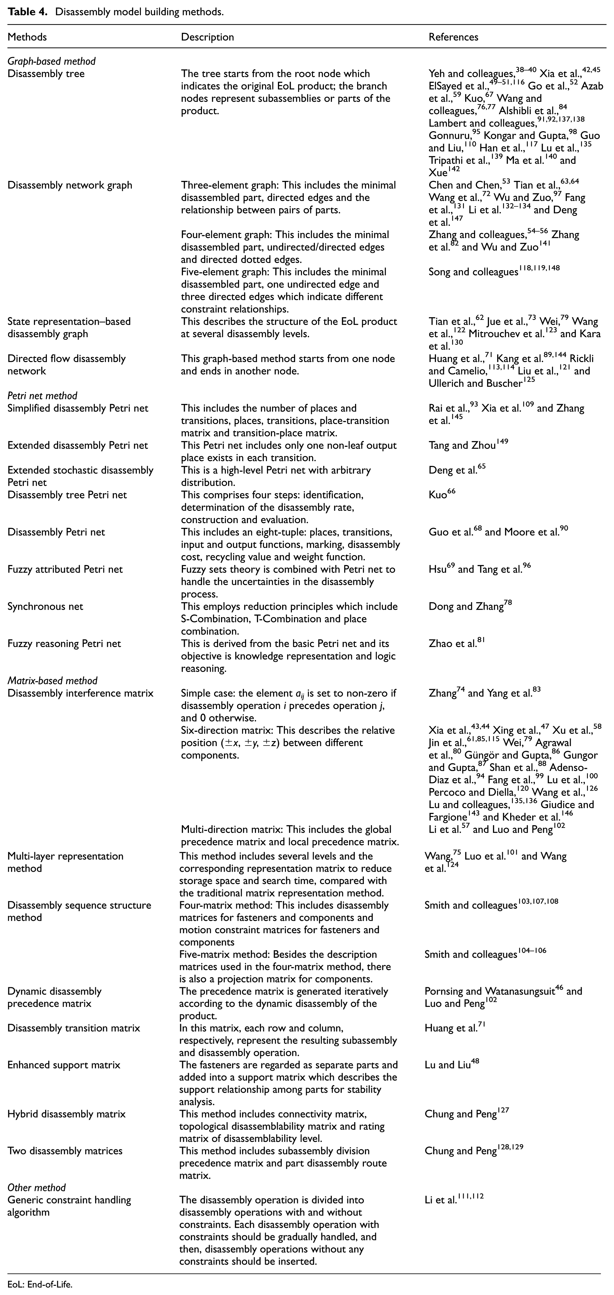
EoL: End-of-Life.

Graphs

The use of disassembly trees was proposed by Bourjault.¹⁵⁰ The tree starts from the root node which indicates the original EoL product. The branch nodes represent subassemblies or parts of the product.³⁸ As shown in Figure 3, R indicates the original product, while S represents a subassembly. Through disassembly (directed edges in Figure 3), different subassemblies are generated

G = {V, E, Ra}

(1)

Disassembly network graphs are used to describe the structural relationships between parts. According to different descriptions of the constraint relationships, a disassembly network graph as shown in Figure 4 can be a three-element, four-element or five-element graphs. The minimal part in a disassembly network graph is a component or a connection. A three-element disassembly network graph is described by equation (1),⁵³ where G is the disassembly network graph, V represents the minimum part, E_ij is the directed edge from i to j indicating that component i should be disassembled before component j, Ra is a set of arcs (an actual arc stands for an ‘AND’ relationship and a virtual arc means an ‘OR’ relationship between different parts). Using this method, the structural relationship between different parts can be clearly described. However, the relationships between different parts cannot be simply represented as ‘AND’ or ‘OR’ relationships, the precedence relationship between contact components and non-contact components should also be considered. Thus, in addition to elements V and E, a four-element disassembly network graph includes the relationship sets E_fc and E_c which are, respectively, described as directed solid edge and directed dotted edge.^54,55,82E_fc and E_c, respectively, give the disassembly precedence relationship between contact parts and that between non-contact parts. Song and colleagues.^118,119 added a selective constraint set to the four-element disassembly network graph to provide further structural relationship information and give a five-element disassembly network graph. A part belongs to the selective constraint set if it has constraint relationships with many other parts and can be disassembled once one of those parts is removed.

Figure 3.

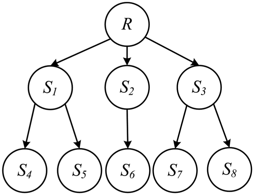
A disassembly tree.

Figure 4.

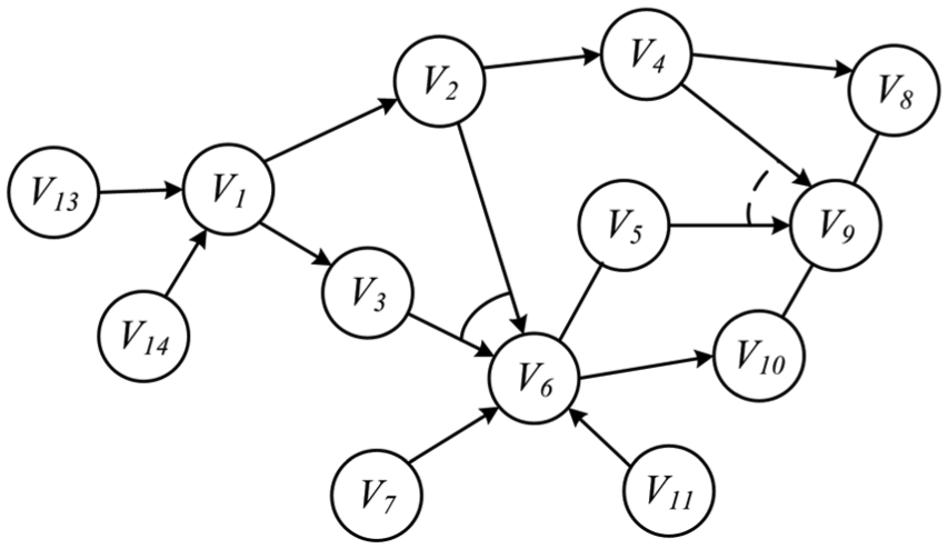
Disassembly network graph.

A state-representation-based disassembly graph describes the structural relationships of a product at different levels or disassembly stages.⁶² With this method, several parts are disassembled during each disassembly stage (in Figure 5(a)) or disassembly level (in Figure 5(b)). The method provides good visualisation of the disassembly process and can also be applied to complex products. Tian et al.⁶² used disassembly models similar to that depicted in Figure 5(b), but ignored details such as disassembly direction. As mentioned previously, to remedy this, Mitrouchev et al.¹²³ used sets of disassembly of removal (SDR) to obtain the possible removal directions for each component. From the SDR, the detachability of each component can be determined.

Figure 5.

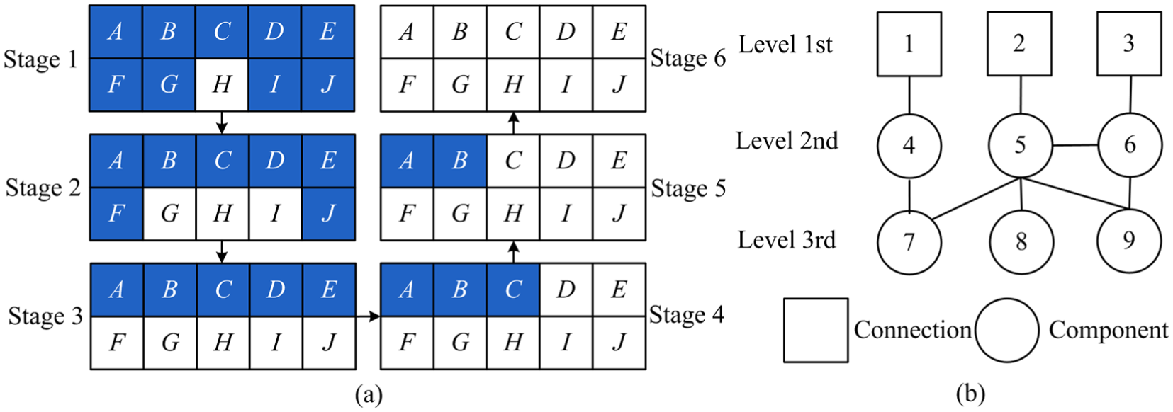
State-representation-based disassembly graph: (a) disassembly stages and (b) disassembly levels.

Unlike a disassembly network graph, a directed flow disassembly network¹¹³ starts from one node which stands for the assembled product and ends at another node which represents the complete disassembly of all parts,¹¹⁴ as shown in Figure 6. However, disassembly details (such as disassembly time, tool and direction) are usually ignored in this method. To address this, Liu et al.¹²¹ included a feasibility graph which not only describes the constraint and adjacency relationships between different parts or subassemblies but also contains other disassembly information (disassembly tool, time, etc.). The optimal disassembly sequence (bold arrows in Figure 6) can be chosen from the available solutions.

Figure 6.

Directed flow disassembly network.

Petri net methods

Xia et al.¹⁰⁹ used the simplified disassembly Petri net method which was defined as a five-tuple as shown in equation (2)

DPN = (P, T, I_{n * m}, O_{m * n}, M)

(2)

where P and T, respectively, represent the sets of EoL products (named places) and disassembly operators (named transitions), n and m are, respectively, the number of places and transitions, matrix I and matrix O, respectively indicate the place-transition matrix and transition-place matrix, M represents the disassembly state of the product. Similarly, a simplified representation of the disassembly Petri net approach was presented, which included places P, transitions T and arcs.⁶⁶ An eight-tuple disassembly Petri net was also used to describe the geometric constraint relationships, removal states and AND/OR logical relationships of all the components.⁶⁸ In addition, to provide rich descriptions of the disassembly structure, as shown in Figure 7, the five elements of the simplified disassembly Petri net method¹⁰⁹ were supplemented with the removal cost c and reuse value of components and the set of weight functions w related to the transition. Based on the standard Petri net, a higher level Petri net, the ‘Extended stochastic disassembly Petri net’ was proposed.⁶⁵ In this method, parameters related to the disassembly process such as the disassembly time probability density functions of the transition, the quality condition function and the probability value of the transition were included.

Figure 7.

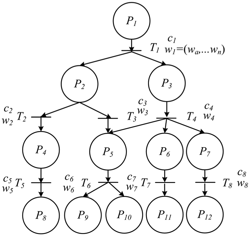
Disassembly Petri net.

Traditional disassembly Petri net methods have disadvantages of complex reachability graph generation and heavy computational burden. When EoL products have complex structures, it is difficult and can take long time to generate the reachability graph. Dong and Zhang⁷⁸ proposed a disassembly model based on a synchronous net to simplify the Petri nets. Through reduction principles, the complex reachability graph problem is solved. In addition, the traditional disassembly Petri net method is not robust enough to handle uncertainties during disassembly process. Compared with traditional Petri net models, the predicate/transition net which is a high-level Petri net was developed to have a compact size and powerful modelling capability. A novel high-level Petri net, the ‘Fuzzy attributed and timed predicate/transition net’ (FATP/T), was developed to deal with uncertainty problems.⁶⁹ The Fuzzy Reasoning Petri net (FRPN) proposed by Zhao et al.⁸¹ handles uncertainty problems in a different way from FATP/T. Apart from the basic elements of a disassembly Petri net, FRPN also incorporates rules with associated confidence levels to enable knowledge-based reasoning and decision making to address the problem of combinational explosion. Petri net was also combined with Bayesian learning to deal with the uncertainties in the disassembly process to reduce the impact of inaccuracy of decision making.¹⁴⁹

Matrix-based methods

Matrix-based methods use several matrices to describe the disassembly precedence relationships between different parts. The disassembly interference matrix method is the most common matrix-based method. The simplest way of constructing a disassembly interference matrix was described in publications.^74,83 With this method, regardless of details such as disassembly directions and disassembly operations, if component i should be disassembled before component j, element b_ij of the disassembly interference matrix is non-zero. Otherwise, it is ‘0’. However, actual disassembly process is more complex due to non-ignorable factors such as disassembly directions and disassembly tools. Based on the CAD model of the product, disassembly interference matrices (C_X+, C_X−, C_Y+, C_Y−, C_Z+, C_Z−) can be generated in six directions (X+, X−, Y+, Y−, Z+, Z−) according to the spatial interference relationship between different parts.⁴⁷ If there is spatial interference between parts i and j along a specific direction, element b_ij of the disassembly interference matrix is ‘1’ in that direction. Otherwise, it is ‘0’. After the disassembly interference matrices of all the directions are obtained, the feasible disassembly sequence can be generated. However, connections are different from components in the actual disassembly process. Therefore, according to the same interference rules mentioned above,^43,44,120 the disassembly interference matrices of components and connections were, respectively, introduced as independent matrices which are row-column matrices and disassembly interference matrices.^42–44 However, the actual disassembly directions of parts are not always the simple six directions (X+, X−, Y+, Y−, Z+, Z−) but could be complex directions. They may change with different structures of components, which results in the previously mentioned methods not meeting the requirements of actual disassembly situations. The extended interference matrix method was proposed to handle those situations.^57,102 With this method, a global coordinate system and a local coordinate system were simultaneously used to increase the diversity of disassembly directions. The global coordinate system was employed to describe interference relationships between components viewed from a common frame of reference, while the local coordinate system was adopted to describe the disassembly interference from the perspective of individual components. The translating and rotating relationships between the global coordinate system and local coordinate system were used to establish the extended interference matrix method.

As with the methods used in publications,^43,44,120 the connections and components were considered separately by different description methods. Smith and colleagues^103,107 proposed the disassembly sequence structure method to represent the spatial relationships between components and connections. With this method, the disassembly matrices for components and connections (two matrices) and the disassembly motion matrices for components and connections (two matrices) were simultaneously built. The disassembly matrices were used to record the disassembly direction of each part, and the disassembly motion matrices, to record touching parts that constrain the disassembly of target components in specific directions. This method helps to reduce model complexity compared with other matrix-based methods. By adding the projection matrix for the components, Smith and colleagues.^104–106 proposed the five-matrix disassembly sequence structure method. Besides the four-matrix method,^103,107 the projection matrix for the components was used to record the number of blocking components for each component. Compared with the four-matrix disassembly sequence structure method, this method further decreases the time to search for feasible sequence solutions. An obvious disadvantage of these method is that the matrices should be generated manually which may be a cumbersome task.

The disassembly interference matrix method needs to record all the relationships of parts even if there are no precedence relationships between them, which naturally results in data redundancy. To reduce processing time and data size, the multi-layer representation method was proposed.^75,101 The Bill-of-Materials (BoM) represented by a list of elements from the product all the way down to basic components was used to generate the natural structure of the product which comprises different layers and nodes. For every subassembly of each layer, a matrix was used to describe the constraints between different components of the subassembly. Compared with the disassembly interference matrix, this method needs a smaller space to store the product model.¹⁰¹

The above-mentioned methods are static description methods because they cannot be altered dynamically according to the actual disassembly situation. To deal with changing conditions, the dynamic disassembly precedence matrix was proposed.^46,102 Based on the same rules,⁷⁴ the disassembly interference matrix was iteratively updated through the following rule: if all elements in column i are 0, then component i will be disassembled, after which, all the elements in row i of the disassembly interference matrix will be set to 0.⁴⁶ Slightly different from the method of publication,⁴⁶ component i should be disassembled if there is only a non-zero element in column (or row) i, after which, the corresponding row i and column i are deleted dynamically.¹⁰²

In terms of disassembly operations and support relationships, there also exist matrix-based methods that are different from the above. The disassembly transition matrix considered the disassembly operation to form a disassembly transition matrix of which the column and row, respectively, represent the disassembly operation and resulting subassembly.⁷¹ An obvious disadvantage of this method is that all the feasible subassemblies and disassembly operations should be enumerated, which is a time-consuming process. Because actual disassembly operations are affected by gravity, to be closer to real situations, the enhanced support matrix was proposed.⁴⁸ The base component supporting other parts or fasteners was determined first and then the support relationships between different components were considered. Furthermore, the hybrid disassembly matrix¹²⁷ and two disassembly matrices^128,129 were also studied.

Other methods

To propose a universal method to handle various disassembly models, the generic constraint handling algorithm was proposed by Li et al.^111,112 Disassembly operations are divided into two parts: those with and those without constraints. First, the positions of disassembly operations without any constraints should be kept unchanged. Then, the element positions of disassembly operations with constraints should be adjusted according to the disassembly precedence relationships. A feasible disassembly sequence will be obtained after all the positions of disassembly operations with constraints have been adjusted. To be a generic constraints description method, the algorithm ignores many details such as the tools used and the disassembly directions which are important for disassembly.

Regarding disassembly model building methods, graphs (58 papers) are the most common methods to build the disassembly model, followed by matrix-based method (40 papers). Graphs give an intuitive way to describe precedence and contact information among the parts of an EoL product. Matrix-based methods provide a more convenient means for the computer to handle disassembly constraint relationships. For matrix-based methods, redundant data are a common problem faced by existing description methods, as most of the methods need to record the relationships between all parts even when no such relationships exist. On the contrary, Petri nets (12 papers) give detailed geometrical and topological information on the components of the EoL product. It has been noted that the actual disassembly process is full of uncertainties and randomness. At the end of its service life, a product may not have a structure consistent with its original structure, which leads to deviations from the disassembly model. Moreover, most disassembly model building methods are static methods. To handle uncertainties caused by unplanned problems such as damaged or missing parts, disassembly models must be capable of dynamic adjustment.

Planning methods

After the disassembly mode and disassembly model have been determined for a given EoL product, planning methods should be used to find the optimal solution from various alternatives. This section covers existing planning methods from two points of view: disassembly objectives (section ‘Disassembly objective’) and optimisation methods (section ‘Optimisation methods’).

Disassembly objective

This deals with the criteria for the optimal disassembly plan (low cost, low environmental impact or high revenue). After the disassembly models are created, specific disassembly objectives are described to make the optimisation process move in specific directions. In the reviewed articles, disassembly objectives are summarised as shown in Table 5. From Table 5, it can be seen that the disassembly objectives are divided into four approaches: disassembly cost, disassembly revenue, environmental indices and other indices.

Table 5.

Disassembly objectives.

Disassembly objectives		Description	References
Disassembly cost objectives
Disassembly time	Basic disassembly time	Time required for disassembling a regular component	Yeh,^38,39 Chen et al.,⁴¹ Xia et al.,⁴² Pornsing and Watanasungsuit,⁴⁶ ElSayed et al.,^49,50,116 Go et al.,⁵² Zhang and colleagues,^54–56 Azab et al.,⁵⁹ Hsu,⁶⁹ Zhang,⁷⁴ Wang,⁷⁵ Tang et al.,⁹⁶ Luo and colleagues,^101,102 Smith et al.,¹⁰⁸ Li et al.,^111,112 Jin et al.,¹¹⁵ Song and colleagues,^118,119 Percoco and Diella,¹²⁰ Wang et al.,¹²⁴ Giudice and Fargione¹⁴³ and Kang et al.¹⁴⁴
	Additional disassembly time	Extra time caused by issues such as geometric complexity and process complexity	Wang⁷⁵ and Luo and colleagues^101,102
	Direction-change disassembly time	Extra time required to change directions of movement during disassembly	Yeh and colleagues,^38–40 Chen et al.,⁴¹ Xia et al.,^42–44 Pornsing and Watanasungsuit,⁴⁶ Xing et al.,⁴⁷ Lu and Liu,⁴⁸ Go et al.,⁵² Chen and Chen,⁵³ Li et al.,⁵⁷ Xu et al.,⁵⁸ Azab et al.,⁵⁹ Kheder et al.,^60,146 Jue et al.,⁷³ Wang,⁷⁵ Dong and Zhang,⁷⁸ Agrawal et al.,⁸⁰ Zhang et al.,⁸² Yang et al.,⁸³ Güngör and Gupta,⁸⁶ Gungor and Gupta,⁸⁷ Shan et al.,⁸⁸ Moore et al.,⁹⁰ Adenso-Diaz et al.,⁹⁴ Wu and Zuo,^97,141 Kongar and Gupta,⁹⁸ Fang et al.,⁹⁹ Lu et al.,¹⁰⁰ Smith and colleagues,^{103–105,107,108} Guo and Liu,¹¹⁰ Jin et al.,¹¹⁵ Percoco and Diella,¹²⁰ Wang et al.,¹²⁶ Li et al.,^132,134 Xue,¹⁴² Giudice and Fargione,¹⁴³ Zhang et al.,¹⁴⁵ Deng et al.¹⁴⁷ and Mi et al.¹⁵¹
	Tools-change disassembly time	Time required for changing tools	Yeh and colleagues,^38–40 Chen et al.,⁴¹ Xia et al.,^42–44 Lu and Liu,⁴⁸ ElSayed et al.,^49–51,116 Go et al.,⁵² Chen and Chen,⁵³ Zhang et al.,⁵⁵ Li et al.,⁵⁷ Xu et al.,⁵⁸ Azab et al.,⁵⁹ Kheder et al.,^60,146 Wang et al.,⁷² Jue et al.,⁷³ Zhang,⁷⁴ Dong et al.,⁷⁸ Agrawal et al.,⁸⁰ Zhang et al.,⁸² Yang et al.,⁸³ Alshibli et al.,⁸⁴ Güngör and Gupta,⁸⁶ Gungor and Gupta,⁸⁷ Shan et al.,⁸⁸ Moore et al.,⁹⁰ Adenso-Diaz et al.,⁹⁴ Wu and Zuo,^97,141 Kongar and Gupta,⁹⁸ Fang et al.,⁹⁹ Lu et al.,¹⁰⁰ Smith et al.,¹⁰⁸ Guo and Liu,¹¹⁰ Li et al.,^132,134 Lu and colleagues,^135,136 Xue,¹⁴² Zhang et al.,¹⁴⁵ Deng et al.¹⁴⁷ and Mi et al.¹⁵¹
	Travelling time between different disassembly points	Time for moving between different disassembly points	ElSayed et al.,^49–51,116 Azab et al.⁵⁹ and Alshibli et al.⁸⁴
	Stochastic time	Disassembly times are stochastically distributed	Yeh et al.⁴⁰ Chen,⁵³ Tian et al.,^62–64 Deng et al.⁶⁵ and Kuo⁶⁶
	Fuzzy time	Disassembly times are represented as triangular fuzzy numbers	Zhang et al.⁷⁰
Disassembly tooling cost		Cost of tooling for disassembly operation	Xia et al.,⁴³ Kuo,⁶⁶ Guo and colleagues,^68,110 Zhang et al.,⁷⁰ Wang et al.,⁷² Wang et al.,^76,77 Kang et al.,⁸⁹ Lambert and colleagues,^91,137,138 Gonnuru,⁹⁵ Smith et al.,¹⁰⁸ Rickli and Camelio,^113,114 Han et al.,¹¹⁷ Song and colleagues,^118,119 Ullerich and Buscher,¹²⁵ Chung and Peng,¹²⁹ Lu et al.,¹³⁵ Tripathi et al.,¹³⁹ Ma et al.¹⁴⁰ and Giudice and Fargione¹⁴³
Labour cost		Cost of disassembling an EoL product per time unit	Pornsing and Watanasungsuit,⁴⁶ Tian et al.,^63,64 Deng et al.,⁶⁵ Kuo,⁶⁶ Hsu,⁶⁹ Tang et al.,⁹⁶ Smith et al.,¹⁰⁸ Jin et al.,¹¹⁵ Song and colleagues,^118,119 Percoco and Diella,¹²⁰ Ullerich and Buscher¹²⁵ and Kang et al.¹⁴⁴
Parts number		Total number of parts disassembled	Xing et al.,⁴⁷ Lu and Liu,⁴⁸ Kheder et al.,⁶⁰ Agrawal et al.,⁸⁰ Gungor and Gupta,⁸⁶ Luo et al.,¹⁰¹ Smith and colleagues,^103,107,108 Jin et al.,¹¹⁵ Wang et al.¹²⁶ and Deng et al.¹⁴⁷
Operation number		The total number of operations in the disassembly process	Chung and Peng¹²⁹
Disassembly distance		Distance moved in disassembling a component	Xing et al.⁴⁷
Maintenance degree		Type of maintenance required (no maintenance, corrective maintenance or preventive maintenance)	Kheder et al.^60,146
MTTR		Calculated by the summation of mean time to repair of each part	Chung and Peng¹²⁷
Disassembly revenue objectives
Components revenue	Non-destructive disassembly revenue of a component	Revenue for a salvaged component undamaged by disassembly	Chen and Chen,⁵³ Kuo,⁶⁶ Guo et al.,^68,110 Hsu,⁶⁹ Kang et al.,^89,144 Lambert and colleagues,^{91,92,137,138} Gonnuru,⁹⁵ Tang et al.,⁹⁶ Smith et al.,¹⁰⁸ Rickli and Camelio,¹¹⁴ Jin et al.,¹¹⁵ Ullerich and Buscher,¹²⁵ Lu et al.¹³⁵ and Ma et al.¹⁴⁰
Components revenue	Destructive disassembly revenue of a component	Revenue for a component damaged by disassembly	Smith et al.¹⁰⁸ and Guo and Liu¹¹⁰
Recovered weight (or volume)		Weight (or volume) of each component	Xia et al.,^45,109 Pornsing and Watanasungsuit,⁴⁶ Chen and Chen,⁵³ Kuo,⁶⁶ Li et al.,^111,112 Jin et al.,¹¹⁵ Smith et al.,¹⁰⁸ Ullerich and Buscher,¹²⁵ Tripathi et al.,¹³⁹ Kang et al.¹⁴⁴ and Kheder et al.¹⁴⁷
Recovered value		A function of the reuse value of each reusable component and the recycling value of each recyclable component	Xia et al.,^45,109 Pornsing and Watanasungsuit,⁴⁶ Chen and Chen,⁵³ Kuo,^66,67 Gungor et al.,^86,87 Kongar et al.,⁹⁸ Li et al.,^111,112 Jin et al.¹¹⁵ and Tripathi et al.¹³⁹
Dynamic product value		Product value modelled as a negative exponential function of time	Rickli and Camelio¹¹⁴
Profit probability		Profit probability of a disassembly sequence	Rickli and Camelio¹¹⁴
Environmental objectives
Environmental impact of a component		Effect of a component on the environment	Xia et al.,^45,109 Pornsing and Watanasungsuit,⁴⁶ Kuo,⁶⁷ Güngör and Gupta,⁸⁶ Gungor and Gupta,⁸⁷ Moore et al.,⁹⁰ Gonnuru,⁹⁵ Smith et al.,¹⁰⁸ Li et al.,^111,112 Rickli and Camelio,¹¹³ Jin et al.,¹¹⁵ Percoco and Diella,¹²⁰ Ullerich and Buscher,¹²⁵ Tripathi et al.,¹³⁹ Ma et al.¹⁴⁰ and Giudice and Fargione¹⁴³
Environmental impact of a disassembly operation		Effect of a disassembly operation on the environment	Rickli and Camelio¹¹³
Other objectives
Feasibility		Index relating to the feasibility of a disassembly sequence	Rickli and Camelio^113,114
Stability		Index relating to the stability of components connected in a particular way (soldering, welding, riveting, screwing)	Lu and Liu,⁴⁸ Yang et al.⁸³ and Deng et al.¹⁴⁷

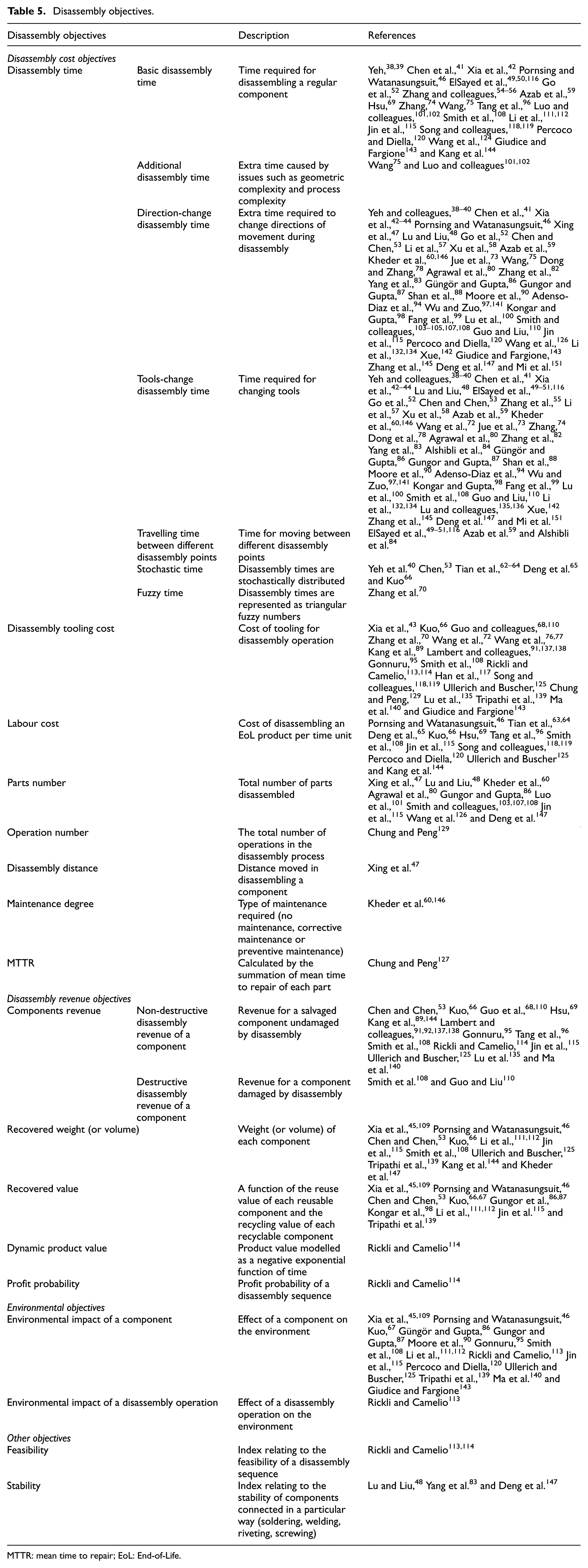
MTTR: mean time to repair; EoL: End-of-Life.

From Table 5, it can be noted that the disassembly cost objective is sub-divided into disassembly time, disassembly tooling cost, labour cost, parts number, operation number, disassembly distance and maintenance degree. The basic disassembly time is the time required for disassembling a regular component. However, the actual disassembly time for removing a component is not a constant value because it is influenced by other factors. To distinguish the disassembly times for operations with different degrees of difficulty, the idea of additional disassembly time was proposed.^75,101,102 The additional disassembly time was combined with the basic disassembly time to be variable disassembly time. The additional disassembly time still does not take into account practical factors such as tool changes, direction changes and time for travelling between disassembly points. Researchers have supplemented the additional disassembly time with further allowances for tool changes, direction changes and movements between disassembly points. Tool changes incur time penalties for obvious reasons. In the case of direction changes, the larger the disassembly direction changes, the larger the penalty. In the reviewed papers, the time to travel between disassembly points is normally calculated using the Euclidean distance between different disassembly points and the speed of the transfer equipment (e.g. a robot arm). However, in practice, the actual disassembly time for a component depends not only on the aforementioned deterministic time elements but also on uncertainties in the disassembly process. Stochastic disassembly times⁵³ and fuzzy times⁷⁰ have been proposed to deal with those uncertainties. Depending on the problem, the randomly varying (stochastic) time for removing a component could be taken as normally distributed or Gaussian distributed, whereas triangular numbers have been adopted to represent imprecise (fuzzy) disassembly time. Apart from disassembly time, the cost of tooling should also be considered. Tooling cost means the cost of tooling for disassembly operations such as the cost of torches and wrenches screwdrivers. In cases where manual disassembly is adopted to deal with uncertainties in the disassembly process, labour costs become a consideration.⁴⁶ Other factors affecting disassembly costs are the parts number³⁶ the disassembly distance,⁴⁷ maintenance degree,⁶⁰ mean time to repair (MTTR)¹²⁷ and operation number.¹²⁹

The disassembly revenue for a component is also a disassembly objective. Disassembly revenue can also be divided into nondestructive disassembly revenue¹¹⁵ and destructive disassembly revenue¹¹⁰ (again, if a paper does not specify the type of revenue, it is taken as nondestructive disassembly revenue by default). Table 5 shows that the existing literature mainly focuses on nondestructive disassembly revenue. Guo and Liu¹¹⁰ considered the destructive disassembly revenue of a component. However, different destructive disassembly methods will result in different disassembly revenues although no paper so far has discussed this point. With a view to recycling, some authors have considered the recovered weight and recovered value of a component.¹⁰⁹ The above-mentioned objective description methods are static methods. However, in practice, the properties of EoL products can change, among other factors, according to the time they were in use. To account for this dynamic scenario, the product value curve was taken as a negative exponential function of time.¹¹⁴ Apart from these, the profit probability was also studied.¹¹⁴

There has been less work on objectives connected to the environment than on those associated with costs and revenues. Environmental objectives are to reduce environmental impacts of components¹⁰⁹ and of operations.¹¹³ The former concern potential harm by a component and the latter relate to that by a disassembly operation (such as wastage of cleaning fluid or energy). In addition, stability⁴⁸ and feasibility¹¹³ have also been taken as disassembly objectives. Rickli and Camelio¹¹³ used the ratio of feasible arcs over the total number of arcs in a disassembly graph as a feasibility index to be maximised. Other researchers also take into account how stably components are connected together (welding, riveting or press fitting, etc.).⁴⁸

Based on the statistics of publications in Table 5, it can be seen that work related to economic factors (disassembly cost and revenue, 97 papers) has received the most attention. However, considering the importance of environmental factors (18 papers), it is expected that they will attract more research efforts in the future. It is also meaningful to build dynamic economic factors and environmental factors. As stated in section ‘Introduction’, researchers have paid increasing attention to robotic disassembly which helps to promote the automation of disassembly process. When robotic disassembly is considered,⁴⁹ as an important environmental factor, the energy consumption of robots in the disassembly process can also be optimised to promote sustainability.¹⁵² In addition, for robotic disassembly, the trajectory of the robot arm should avoid collision with the product being dismantled. When DSP for robotic disassembly is considered, it is useful to combine obstacle-avoiding path planning with DSP. However, there has been no research on this topic so far.

Optimisation methods

Optimisation methods deal with ways of efficiently finding optimal disassembly sequences. Determining the optimal disassembly sequence under given objectives is an NP-complete problem requiring the use of heuristic algorithms. The main optimisation methods found in the reviewed literature on DSP are nature-inspired heuristic algorithms (NIHA), linear programming methods (LPM), rule-based methods (RBM), stochastic simulation (SSI) techniques and so on.

NIHA

NIHA are derived from natural phenomena such as ants foraging and bees foraging. These algorithms can solve combinatorial optimisation problems. In the reviewed literature of DSP, they are the most common methods to find the optimal disassembly sequences.

In NIHA, GA which is derived from evolution and genetics is the most widely used method to solve disassembly sequence optimisation problems. The disassembly sequences are first coded into chromosomes, and then, the selection, crossover and mutation operators are used to find new chromosomes.⁵² In general, the new chromosomes may not meet the precedence relationship of EoL products. Therefore, GA was combined with precedence-preserving crossover (PPX) in several studies to ensure the feasibility of new chromosomes.^49,60,116 In addition, feasibility (FE) was added to the fitness function of GA.^113,114 For GA, it is easy to be trap at local optimal solutions. To solve this problem, GA with adaptive crossover rate and mutation rate (ACRMR)⁴¹ and GA with Gaussian mutation⁷⁰ were used to improve the quality of solutions. Moreover, simulated annealing (SA)-based GA,⁸³ SA-binary tree (BTA)-based GA,⁹⁷ Tabu search (TS)-based GA¹³⁴ and Chaotic GA (CGA)¹⁴⁵ were also proposed to improve the quality of solutions.

The PSO which is derived from the flocking behaviour of birds is also a common method used for disassembly sequence optimisation. With this method, the velocity and position of particles are updated in each iteration. Pornsing and Watanasungsuit⁴⁶ used the discrete PSO to convert continuous velocity to discrete velocity through sigmoid and round functions. Xu et al.⁵⁸ employed adaptive PSO to avoid premature convergence by using the inertia weight and adaptive mutation rate. To avoid local optima, Li et al.¹¹¹ used the crossover operator, a shift operator and the escaping method to improve the quality of solutions. In addition, simplified swarm optimisation (SSO) is regarded as a type of PSO because the difference between PSO and SSO is only the position update mechanism.³⁸ To ensure global convergence, a revised updating mechanism of simplified swarm optimisation (RUM-SSO) was proposed by dividing the whole population into different groups.⁴⁰ Because the parameters of SSO play vital roles in determining the quality of solutions,³⁸ the self-adaptive parameter control (SPC) method integrated with PPX, feasible solution generator (FSG) and repetitive pairwise exchange method was developed to automatically tune the parameters of SSO.^38,39

The ACO algorithm inspired by the foraging behaviour of ants has also been used to find the optimal disassembly sequence. According to the concentration of pheromone, the ants move to the next permitted destination.¹⁰¹ When the solution space is large enough, it is easy for ACO to converge to local optimal solutions. The max–min ant system was proposed to avoid premature convergence by limiting the concentration of pheromone to a certain range.¹²¹ Execution efficiency of ACO was also studied through a two-stage ACO method.⁷² The first stage ACO was employed to convert complex graph-based method into a simple weighted graph, while the second stage ACO was used to find the optimal disassembly sequence. In addition, a self-guided ant algorithm (ASGA) was proposed to make tradeoff between efficiency and accuracy (Table 6).¹³⁹

Table 6.

Optimisation methods.

Optimisation methods	Descriptions	References
GA
GA	This includes three main steps: selection, crossover and mutation.	Go et al.,⁵² Zhang et al.,⁵⁴ Li et al.,⁵⁷ Zhang,⁷⁴ Wang and colleagues,^75,77 Gonnuru,⁹⁵ Kongar and Gupta,⁹⁸ Chung and Peng,¹²⁹ Li et al.,¹³² Lu and Sun,¹³⁶ Wu and Zuo¹⁴¹ and Giudice and Fargione¹⁴³
GA-PPX	GA and precedence-preserving crossover are simultaneously used.	ElSayed et al.,^49–51,116 Kheder et al.⁶⁰ and Agrawal et al.⁸⁰
GA-FE	Feasibility is added into the disassembly objective functions of GA.	Rickli and Camelio^113,114
GA-ACRMR-PPX	Adaptive crossover rate and mutation rate are used to ensure global convergence.	Chen et al.⁴¹
GA-GM	Based on GA, Gaussian mutation operator is included to achieve a better solution.	Zhang et al.⁷⁰
GA-SA	SA is used after the mutation operation to achieve better performance.	Yang et al.⁸³
GA-SA-BTA	Binary tree and SA are combined with the GA.	Wu and Zuo⁹⁷
GA-TS	Tabu search is integrated with GA.	Li et al.¹³⁴
CGA	Chaotic theory is applied on initial populations and operators of GA.	Zhang et al.¹⁴⁵
PSO
PSO	Velocity and position of each particle are updated in the iteration.	Lu et al.¹³⁵
DPSO	Velocity and position of particles are obtained using the sigmoid function and normal distribution, respectively.	Pornsing and Watanasungsuit⁴⁶
IPSO	Crossover, shift operators and escaping method are used to avoid local optimal solutions.	Jin et al.⁶¹ and Li et al.^111,112
APSO	This dynamically adjusts inertia weight and adaptive mutation rate to avoid local convergence.	Xu et al.⁵⁸
SSO	RUM-SSO: A new updating mechanism is used.	Yeh et al.⁴⁰
	PPX-SSO: This includes PPX, FSG, SPC and repetitive pairwise exchange procedures.	Yeh³⁸
	ISSO: SPC methods and the update mechanism are improved.	Yeh³⁹
ACO
ACO	Ants choose a suitable path by detecting high concentration of pheromone.	Xing et al.,⁴⁷ Wang et al.,⁷⁶ Shan et al.,⁸⁸ Fang et al.,⁹⁹ Lu et al.,¹⁰⁰ Luo and colleagues,¹⁰¹ Wang et al.,¹²⁶ Xue,¹⁴² Kheder et al.¹⁴⁶ and Mi et al.¹⁵¹
IMMAS	The concentration of pheromone is limited to a certain range [τ_min, τ_max].	Liu et al.¹²¹
TSACO	The first stage and second stage, respectively, correspond to operation selection and operation sequencing.	Wang et al.,⁷²
ASGA	This is used to tradeoff between speed and accuracy.	Tripathi et al.¹³⁹
SS
SS-PPX	PPX is integrated with SS to preserve the precedence relationships of new solutions.	Guo and colleagues^68,110
SS-PR	The path-relink combination operator is added to SS.	Guo et al.⁶⁸
ABC
DABC	This is inspired by the foraging behaviour of bees including onlookers, employed bees and scouts.	Percoco and Diella¹²⁰ and Zhang et al.⁸²
IA
AIA	Selection and single-parent mutation operators are used.	Lu and Liu⁴⁸
SA	A hill-climbing search method suitable for solving combinatorial and continuous optimisation problems.	Azab et al.⁵⁹
FFO	This is derived by the foraging behaviour of fruit flies.	Jue et al.⁷³
LPM
BLPM	BLPM of which the decision variables are 0 or 1, is a type of LPM.	Kang et al.^89,144 Lambert and colleagues^{91,92,137,138} Ullerich and Buscher,¹²⁵ and Ma et al.¹⁴⁰
BAB	This consists of setting the upper/lower bounds and branching operations.	Zhang et al.,⁵⁶ Güngör and Gupta⁸⁶ and Han et al.¹¹⁷
RBM
RCM	This reduces searching time and eliminates unrealistic solutions by employing rules.	Smith and colleagues^{103,106–108}
RBM-GA	RBM and GA are used to find optimal solutions of disassembly sequence.	Smith and colleagues^104,105
SSI
MCS	This can handle the uncertainties in disassembly process.	Chen and Chen⁵³ and Tian et al.⁶³
TPA	Numerical solutions are used to solve stochastic problems based on time and frequency-domain methods.	Tian et al.⁶²
NN-SSI	Based on SSI, part of data is the training set and the remaining is the testing set of neural network.	Tian et al.⁶⁴ and Deng et al.⁶⁵
GA-NN-SSI	Based on SSI, GA is used to optimise weight and thresholds of neural network.	Tian et al.⁶⁴
STLBA	This comprises an FSG, a teaching phase operator and a learning phase operator.	Xia et al.^42–45
EM	This enumerates all possible solutions and finds the best one.	Luo et al.,¹⁰² Jin et al.¹¹⁵ and Wang et al.¹²² and Wang et al.¹²⁴
OIM	It is used to obtain the shortest disassembly path to the target object.	Song and colleagues^118,119
QL	This includes state and action, the disassembly state matrix is updated through actions.	Xia et al.¹⁰⁹
FRS	This encapsulates the fuzzy sets and rough sets to solve DSP problem.	Zhang et al.⁵⁵
TS	This consists of short- and long-term memories, which are used, respectively, to prevent reversal and reinforce attractive components.	Alshibli et al.⁸⁴
GRASP	The solution construction step and local search step are included in GRASP.	Adenso-Diaz et al.⁹⁴
DA	A typical algorithm to solve the shortest path problem.	Lu et al.¹³⁵

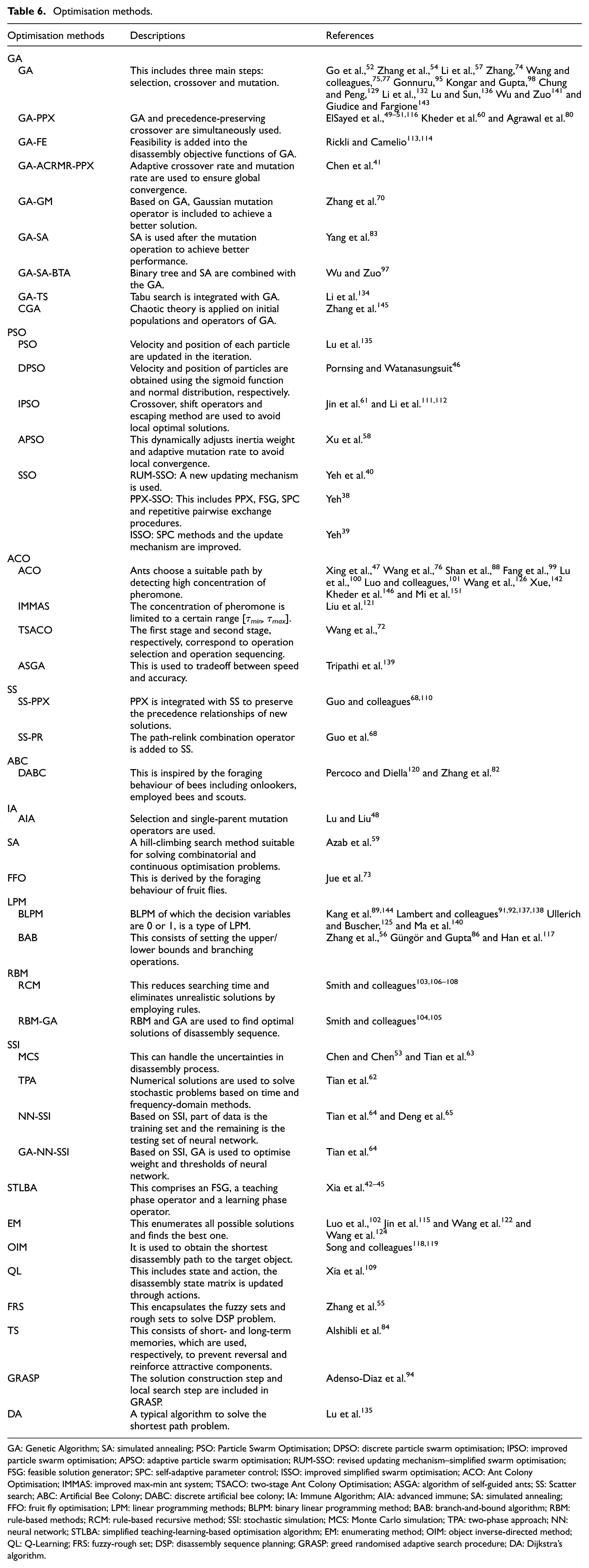
GA: Genetic Algorithm; SA: simulated annealing; PSO: Particle Swarm Optimisation; DPSO: discrete particle swarm optimisation; IPSO: improved particle swarm optimisation; APSO: adaptive particle swarm optimisation; RUM-SSO: revised updating mechanism–simplified swarm optimisation; FSG: feasible solution generator; SPC: self-adaptive parameter control; ISSO: improved simplified swarm optimisation; ACO: Ant Colony Optimisation; IMMAS: improved max-min ant system; TSACO: two-stage Ant Colony Optimisation; ASGA: algorithm of self-guided ants; SS: Scatter search; ABC: Artificial Bee Colony; DABC: discrete artificial bee colony; IA: Immune Algorithm; AIA: advanced immune; SA: simulated annealing; FFO: fruit fly optimisation; LPM: linear programming methods; BLPM: binary linear programming method; BAB: branch-and-bound algorithm; RBM: rule-based methods; RCM: rule-based recursive method; SSI: stochastic simulation; MCS: Monte Carlo simulation; TPA: two-phase approach; NN: neural network; STLBA: simplified teaching-learning-based optimisation algorithm; EM: enumerating method; OIM: object inverse-directed method; QL: Q-Learning; FRS: fuzzy-rough set; DSP: disassembly sequence planning; GRASP: greed randomised adaptive search procedure; DA: Dijkstra’s algorithm.

SS is a systematic integrated method which includes diversification generation, solution improvement, reference set updating, subset generation and solution combination. It can achieve a balance between quality and diversity of solutions by forming high-quality solution sets and diverse solution sets. Guo and Liu¹¹⁰ used the PPX to preserve disassembly precedence relationships from one generation to the next based on SS. After that, Guo et al.⁶⁸ continued to use the path-relink combination operator to disassemble large and complex products.

The Immune Algorithm (IA) and ABC have also been used to solve DSP. The selection operator and the single-parent mutation operator were adopted to ensure the diversity and quality of the antibodies.⁴⁸ A transition rule was added in the discrete artificial bee colony (DABC) algorithm to generate new candidate solutions which helps to find the optimal disassembly solution more quickly.¹²⁰ Other methods such as SA⁵⁹ and fruit fly optimisation (FFO)⁷³ have also been used. They are not so commonly used, and thus will not be discussed in detail.

LPM

LPM is popular method for solving constrained extremum problems. The binary linear programming method (BLPM) is a type of LPM with decision variable that is either 1 or 0.⁸⁹ Compared with the integer LPM, BLPM helps to improve efficiency by using a simplified representation.⁹¹ However, it is difficult to employ BLPM to solve complicated DSP problems. The branch-and-bound algorithm (BAB) was also used to solve linear programming problems.¹¹⁷ BAB finds the optimal disassembly sequence by setting the upper/lower bounds and branching operations. To improve the efficiency of BAB, Güngör and Gupta⁸⁶ used two user-defined variables to reduce the search space and the number of nodes.

SSI

SSI is an efficient method of finding the optimal disassembly sequence of a stochastic disassembly process. Monte Carlo simulation (MCS) was used to obtain the optimal disassembly sequence with stochastic disassembly time.^53,63 However, this method, which has the disadvantages of low accuracy and low efficiency, is easily influenced by the sample size. Tian et al. used a two-phase approach to address this problem. Disassembly probability density functions were generated by a time-domain or frequency-domain procedure.⁶² Furthermore, neural network (NN)⁶⁴ and GA-NN-based SSI⁶⁴ were also proposed to find optimal disassembly sequences with stochastic disassembly costs.

RBM

Smith and colleagues^{103,106–108} used rules to eliminate unrealistic solutions and generate feasible disassembly sequences. With this method, five rules are iteratively checked until the target component is obtained to produce a feasible disassembly sequence under the partial disassembly mode. After that, Smith and colleagues^104,105 continued to combine RBM with GA to solve the DSP. Based on the disassembly sequence structure method (five-matrix method), Smith used RBM and GA to reduce the search time by narrowing the search space to find the optimal disassembly sequence. Compared with other methods, this reduces the search time by adding a projection matrix of components.¹⁰³

Simplified teaching-learning-based optimisation

Although NIHA performs well in disassembly sequence optimisation problems, it is essential to use suitable parameters under specific cases, which makes it insufficiently robust for different situations. Under this condition, a simplified teaching-learning-based optimisation algorithm (STLBA) was applied in DSP.^42–44 Its obvious advantage is that there is no need to tune the input parameters of STLBA to achieve the optimisation goal. Together with FSG, STLBA includes the teaching phase operator, which is used to improve the mean of learners’ results, and a learning phase operator, which is used to learn from each other. STLBA can solve complex combinatorial optimisation problems through fewer input parameters than NIHA.

Other methods

Apart from the optimisation methods mentioned before, a reinforcement value was added to the Q-learning method (QL) to achieve the optimisation goal with a smaller number of disassembly operations.¹⁰⁹ Enumerating methods (EM) were also used to solve small-to-medium-sized problems.^102,115,124 When a complicated model is used, the processing time increases exponentially, which makes EM incapable of dealing with complex situations. In addition, the object inverse-directed method (OIM) is mainly used in the partial disassembly mode to generate the optimal disassembly solution.¹¹⁸

Other methods such as fuzzy-rough set (FRS),⁵⁵ TS,⁸⁴ greed randomised adaptive search procedure (GRASP)⁹⁴ and Dijkstra’s algorithm (DA)¹³⁵ were also used in DSP. They are not so commonly used, thus will not be discussed in detail.

Regarding optimisation methods, there have been many publications on NIHA. GA (27 papers) is the most frequently used method in NIHA, followed by ACO (13 papers). Most NIHA research has focused on improving either solution quality or efficiency. Different from NIHA of which the performance relies on the input parameters, STLBA was proposed to solve DSP without parameter adjustment.⁴² This makes STLBA easier to apply and it is expected to gain popularity in the future. However, most planning methods are static methods and the obtained results may not be usable in practice due to uncertainties in the disassembly process. To make optimisation results more suitable for practical applications, it is important to develop disassembly sequence re-planning methods to update the optimal disassembly sequence in response to the actual state of the disassembly. However, there is no research in this regard. In recent years, deep reinforcement learning, as a promising artificial intelligence method, has been paid increasing attention.^153,154 However, so far, there is no research using deep reinforcement learning to solve DSP problems involving uncertainties. This is an opportunity for researches in the area of disassembly planning.

Finally, as it is likely that, in the short to medium term, disassembly cannot economically be carried out entirely by robots. Humans are still required to perform difficult disassembly tasks involving high degrees of uncertainty. In addition, to finish complicated tasks flexibly, human–robot collaboration^155,156 combines robot efficiency and human adaptability.¹⁵⁷ Human–robot collaborative systems have successfully been applied in the field of cellular manufacturing.^158,159 More work would need to be done on how to find optimal disassembly sequences for situations when humans and robots work together.

Conclusion and future trends

This article has reviewed the state-of-the-art of DSP research from perspectives that encompass the process of disassembly for remanufacturing: disassembly mode, disassembly modelling and planning methods. This section summarises the results of the review and suggests areas for further study in this field.

The main conclusions are that (1) most researchers have focused on complete and sequential disassembly; (2) most pre-processing methods are manually finished only if CAD models of EoL products are provided; (3) most disassembly model building methods are static methods and cannot dynamically adapt to uncertainties in the disassembly process; (4) most researchers have considered economic factors and only a few have investigated environmental factors; (5) deterministic objectives are more frequently studied compared with stochastic and fuzzy objectives; (6) most optimisation methods have focused on NIHA; and (7) much attention has been paid to off-line optimisation methods.

Future work in this field could include the following: (1) further research on parallel and partial/parallel disassembly; (2) development of completely automatic modelling methods to finish pre-processing without CAD models; (3) development of dynamic disassembly modes to handle uncertainties caused by unplanned problems; (4) research into dynamic economic and environmental factors; (5) energy consumption of robots over the whole disassembly process; (6) research that combines DSP with obstacle-avoiding path planning for robots; (7) disassembly sequence re-planning for real disassembly processes; (8) application of deep reinforcement learning to DSP; and (9) DSP for human–robot collaborative disassembly which takes both human adaptability and robot efficiency into consideration.

Footnotes

Appendix 1 Declaration of conflicting interests

The author(s) declared no potential conflicts of interest with respect to the research, authorship and/or publication of this article.

Funding

The author(s) disclosed receipt of the following financial support for the research, authorship, and/or publication of this article: This work was supported by the National Natural Science Foundation of China (Grant Nos. 51775399 and 51475343); Engineering and Physical Sciences Research Council (EPSRC), UK (Grant No. EP/N018524/1); and the China Scholarship Council (Grant No. 201606950054).

ORCID iDs

Wenjun Xu

F Javier Ramirez

References

Guide

VDR

. Production planning and control for remanufacturing: industry practice and research needs. J Oper Manag 2000; 18(4): 467–483.

Duflou

Seliger

Kara

, et al. Efficiency and feasibility of product disassembly: a case-based study. CIRP Ann: Manuf Techn 2008; 57(2): 583–600.

Soh

Ong

Nee

AYC

. Design for disassembly for remanufacturing: methodology and technology. Proc CIRP 2014; 15: 407–412.

Vongbunyong

Kara

Pagnucco

. A framework for using cognitive robotics in disassembly automation. In: Dornfeld

Linke

(eds) Leveraging technology for a sustainable world. Berlin: Springer, 2012, pp.173–178.

Gil

Pomares

Diaz

STPC

, et al. Flexible multi-sensorial system for automatic disassembly using cooperative robots. Int J Comp Integ M 2007; 20(8): 757–772.

Knoth

Brandstotter

Kopacek

, et al. Automated disassembly of electronic equipment. In: IEEE international symposium on electronics and the environment, San Francisco, CA, 6–9 May 2002, pp.290–294. New York: IEEE.

Merdan

Lepuschitz

Meurer

, et al. Towards ontology-based automated disassembly systems. In: IEEE annual conference on industrial electronics society, Glendale, CA, 7–10 November 2010, pp.1392–1397. New York: IEEE.

Vongbunyong

Kara

Pagnucco

. Application of cognitive robotics in disassembly of products. CIRP Ann: Manuf Techn 2013; 62(1): 31–34.

Vongbunyong

Kara

Pagnucco

. Basic behaviour control of the vision-based cognitive robotic disassembly automation. Assembly Autom 2013; 33(1): 38–56.

10.

Vongbunyong

Kara

Pagnucco

. Learning and revision in cognitive robotics disassembly automation. Robot Cim: Int Manuf 2015; 34: 79–94.

11.

Ghoreishi

Jakiela

Nekouzadeh

. A nongraphical method to determine the optimum disassembly plan in remanufacturing. J Mech Design 2013; 135(2): 1–13.

12.

Poli

Kennedy

Blackwell

. Particle swarm optimization. Swarm Intell: US 2007; 1(1): 33–57.

13.

Pham

Castellani

. A comparative study of the Bees Algorithm as a tool for function optimisation. Cogent Eng 2015; 2(1): 1–28.

14.

Karaboga

. An idea based on honey bee swarm for numerical optimization. Report, Erciyes University, Kayseri, October 2005.

15.

Dorigo

Birattari

Stutzle

. Ant colony optimization. IEEE Comput Intell M 2006; 1(4): 28–39.

16.

Qiao

Peng

. An ant colony approach to operation sequencing optimization in process planning. Proc IMeche, Part B: J Engineering Manufacture 2017; 231(3): 470–489.

17.

Zhang

Wang

, et al. An integrated ant colony optimization algorithm to solve job allocating and tool scheduling problem. Proc IMeche, Part B: J Engineering Manufacture 2018; 232(1): 172–182.

18.

Zhang

Yuan

Zhang

. A new discrete double-population firefly algorithm for assembly sequence planning. Proc IMeche, Part B: J Engineering Manufacture 2016; 230(12): 2229–2238.

19.

Sanjeev

Padmanaban

Rajkumar

. Minimizing makespan and total flow time in permutation flow shop scheduling problems using modified gravitational emulation local search algorithm. Proc IMeche, Part B: J Engineering Manufacture 2016; 232(3): 534–545.

20.

Kang

Xirouchakis

. Disassembly sequencing for maintenance: a survey. Proc IMeche, Part B: J Engineering Manufacture 2006; 220(10): 1697–1716.

21.

Lee

Kang

Xirouchakis

. Disassembly planning and scheduling: review and further research. Proc IMeche, Part B: J Engineering Manufacture 2001; 215(5): 695–709.

22.

Lee

Kim

Choi

, et al. Disassembly scheduling: integer programming models. Proc IMeche, Part B: J Engineering Manufacture 2004; 218(10): 1357–1372.

23.

Kim

Jeon

Kim

, et al. Disassembly scheduling with capacity constraints: minimizing the number of products disassembled. Proc IMeche, Part B: J Engineering Manufacture 2006; 220(9): 1473–1481.

24.

Gupta

Erbis

McGovern

. Disassembly sequencing problem: a case study of a cell phone. In: Proceeding of the SPIE international conference on environmentally conscious manufacturing IV, Philadelphia, PA, 26–27 October 2004, pp.43–52. New York: SPIE.

25.

Khoo

Tor

. A novel representation scheme for disassembly sequence planning. Int J Adv Manuf Tech 2002; 20(8): 621–630.

26.

Zhang

Wang

, et al. Single object selective disassembly sequence planning based on ant colony algorithm. Comput Integr Manuf 2007; 13(6): 1109–1114.

27.

Tang

Zhou

Zussman

, et al. Disassembly modeling, planning and application: a review. In: IEEE international conference on robotics and automation, San Francisco, CA, 24–28 April 2000, pp.2197–2202. New York: IEEE.

28.

Hsieh

. Robustness analysis of Petri nets for assembly/disassembly processes with unreliable resources. Automatica 2006; 42(7): 1159–1166.

29.

Kuo

. Disassembly sequence and cost analysis for electromechanical products. Robot Cim: Int Manuf 2000; 16(1): 43–54.

30.

Shimizu

Tsuji

Nomura

. Optimal disassembly sequence generation using a genetic programming. Int J Prod Res 2007; 45(19): 4537–4554.

31.

Kongar

Gupta

. Disassembly sequencing using genetic algorithm. Int J Adv Manuf Tech 2006; 30(5): 497–506.

32.

Zhang

. Product disassembly sequence planning based on particle swarm optimization algorithm. Comput Integr Manuf 2009; 15(3): 508–514.

33.

González

Adenso-Díaz

. A scatter search approach to the optimum disassembly sequence problem. Comput Oper Res 2006; 33(6): 1776–1793.

34.

Laili

Tao

Zhang

, et al. A ranking chaos algorithm for dual scheduling of cloud service and computing resource in private cloud. Comput Ind 2013; 64(4): 448–463.

35.

Laili

Tao

Zhang

, et al. A study of optimal allocation of computing resources in cloud manufacturing systems. Int J Adv Manuf Tech 2012; 63(5–8): 671–690.

36.

Hui

Dong

Duan

. A genetic algorithm for product disassembly sequence planning. Neurocomputing 2008; 71(13): 2720–2726.

37.

Dong

Arndt

. A review of current research on disassembly sequence generation and computer aided design for disassembly. Proc IMeche, Part B: J Engineering Manufacture 2003; 217(3): 299–312.

38.

Yeh

. Optimization of the disassembly sequencing problem on the basis of self-adaptive simplified swarm optimization. IEEE T Syst Man Cyb 2012; 42(1): 250–261.

39.

Yeh

. Simplified swarm optimization in disassembly sequencing problems with learning effects. Comput Oper Res 2012; 39(9): 2168–2177.

40.

Yeh

Lin

Wei

. Disassembly sequencing problems with stochastic processing time using simplified swarm optimization. Int J Innov Manag Tech 2012; 3(3): 226–231.

41.

Chen

Zhang

Liao

. Disassembly sequence planning based on improved genetic algorithm. Adv Intel Soft Compu 2011; 2: 471–476.

42.

Xia

Gao

, et al. Disassembly sequence planning using a simplified teaching–learning-based optimization algorithm. Adv Eng Inform 2014; 28(4): 518–527.

43.

Xia

Gao

Wang

, et al. A simplified teaching-learning-based optimization algorithm for disassembly sequence planning. In: Proceeding of the 2013 IEEE 10th international conference on e-business engineering, Coventry, 11–13 September 2013, pp.393–398. New York: IEEE.

44.

Xia

Gao

Chao

, et al. A cloud-based disassembly planning approach towards sustainable management of WEEE. In: Proceeding of the 2015 IEEE 12th international conference on e-business engineering, Beijing, China, 23–25 October 2015, pp.203–208. New York: IEEE.

45.

Xia

Gao

Wang

, et al. Service-oriented disassembly sequence planning for electrical and electronic equipment waste. Electron Commer R A 2016; 20: 59–68.

46.

Pornsing

Watanasungsuit

. Discrete particle swarm optimization for disassembly sequence planning. In: IEEE international conference on management of innovation and technology, Singapore, 23–25 September 2014, pp.480–485. New York: IEEE.

47.

Xing

Wang

Liu

. Disassembly sequence planning based on Pareto ant colony algorithm. J Mech Eng 2012; 48(9): 186–192.

48.

Liu

. A disassembly sequence planning approach with an advanced immune algorithm. P I Mech Eng C: J Mec 2012; 226(11): 2739–2749.

49.

ElSayed

Kongar

Gupta

, et al. An online genetic algorithm for automated disassembly sequence generation. In: Proceedings of the ASME 2011 international design engineering technical conferences & computers and information in engineering, Washington, DC, 28–31 August 2011, pp.657–664. New York: ASME.

50.

ElSayed

Kongar

Gupta

. A genetic algorithm approach to end-of-life disassembly sequencing for robotic disassembly. In Proceeding of the 2010 Northeast decision sciences institute conference, Alexandria, VA, 26–28 March 2010, pp.402–408. Boston, MA: LRM.

51.

ElSayed

Kongar

Gupta

, et al. A robotic-driven disassembly sequence generator for end-of-life electronic products. J Intell Robot Syst 2012; 68(1): 43–52.

52.

Wahab

Rahman

MNA

, et al. Genetically optimised disassembly sequence for automotive component reuse. Expert Syst Appl 2012; 39(5): 5409–5417.

53.

Chen

. Product disassembly sequence optimization based on profit-probability under uncertain environment. Comput Integr Manuf 2014; 20(4): 793–798.

54.

Zhang

Wang

, et al. Parallel disassembly sequence planning for complex products based on genetic algorithm. J Comp: Aided Des Comp Graph 2015; 27(7): 1327–1333.

55.

Zhang

, et al. Parallel disassembly sequence planning for complex products based on fuzzy-rough sets. Int J Adv Manuf Tech 2014; 72(1): 231–239.

56.

Zhang

. Product cooperative disassembly sequence planning based on branch-and-bound algorithm. Int J Adv Manuf Tech 2010; 51(9): 1139–1147.

57.

Jiang

Wang

. Disassembly sequence planning based on extended interference matrix and genetic algorithm. Comp Eng Des 2013; 34(3): 1064–1068.

58.

Zhang

Fei

. Product remanufacture disassembly planning based on adaptive particle swarm optimization algorithm. J Zhejiang Univ: Sc A 2011; 45(10): 1746–1752.

59.

Azab

Ziout

ElMaraghy

. Modeling and optimization for disassembly planning. Jordan J Mech and Ind Eng 2011; 5(1): 1–8.

60.

Kheder

Trigui

Aifaoui

. Disassembly sequence planning based on a genetic algorithm. P I Mech Eng C: J Mec 2015; 229(12): 2281–2290.

61.

Jin

Xia

. Disassembly matrix for liquid crystal displays televisions. Proc CIRP 2013; 11: 357–362.

62.

Tian

Liu

Tian

, et al. Evaluation model and algorithm of product disassembly process with stochastic feature. Clean Technol Envir 2012; 14(2): 345–356.

63.

Tian

Zhou

Chu

, et al. Probability evaluation models of product disassembly cost subject to random removal time and different removal labor cost. IEEE T Autom Sci Eng 2012; 9(2): 288–295.

64.

Tian

Zhou

Chu

. A chance constrained programming approach to determine the optimal disassembly sequence. IEEE T Autom Sci Eng 2013; 10(4): 1004–1013.

65.

Deng

Qiang

Guo

, et al. Probability evaluation modeling and planning of product disassembly profit. Int J u- e- Serv Sci Technol 2015; 8(9): 327–340.

66.

Kuo

. Waste electronics and electrical equipment disassembly and recycling using Petri net analysis: considering the economic value and environmental impacts. Comput Ind Eng 2013; 65(1): 54–64.

67.

Kuo

. Enhancing disassembly and recycling planning using life-cycle analysis. Robot Cim: Int Manuf 2006; 22(5): 420–428.

68.

Guo

Liu

Zhou

, et al. Disassembly sequence optimization for large-scale products with multiresource constraints using scatter search and Petri nets. IEEE T Cybernetics 2016; 46(11): 2435–2446.

69.

Hsu

. A fuzzy knowledge-based disassembly process planning system based on fuzzy Attributed and timed predicate/transition net. IEEE T Syst Man Cy: S 2017; 47(8): 1800–1813.

70.

Zhang

Feng

Tan

, et al. A novel approach for parallel disassembly design based on a hybrid fuzzy-time model. J Zhejiang Univ: Sc A 2015; 16(9): 724–736.

71.

Huang

Esmaeilian

Behdad

. Multi-purpose disassembly sequence planning. In: Proceeding of ASME 2015 international design engineering technical conferences and computers and information in engineering conference, Boston, MA, 2–5 August 2015, pp.1–9. New York: ASME.

72.

Wang

Fan

. A two-stage ant colony optimization approach based on a directed graph for process planning. Int J Adv Manuf Tech 2015; 80: 839–850.

73.

Jue

Wei

Kemeng

, et al. Guiding disassembly sequence planning based on improved fruit fly optimization algorithm. In: Proceedings of 5th international conference on advanced design and manufacturing engineering, Valencia, 27–29 September 2013, pp.188–194. Valencia: ICADME.

74.

Zhang

. Optimization for disassemble sequence planning of electromechanical products during recycling process based on genetic algorithms. Int J Multim Ubiq Eng 2016; 11(4): 107–114.

75.

Wang

. Disassembly sequence planning for end-of-life products. Master Thesis, University of Manitoba, Winnipeg, MB, Canada, 2016.

76.

Wang

Niu

Xiang

, et al. Ant colony optimization for disassembly sequence planning. In: Proceeding of the ASME 2006 international design engineering technical conferences and computers and information in engineering conference, Philadelphia, PA, 10–13 September 2006, pp.635–641. New York: ASME.

77.

Wang

Xiang

Duan

. A genetic algorithm for product disassembly sequence planning. In: Proceeding of the 2006 IEEE international conference on engineering of intelligent systems, Islamabad, Pakistan, 22–23 April 2006, pp.1–5. New York: IEEE.

78.

Dong

Zhang

. Disassembly sequence planning based on synchronous net. In: Proceeding of the 2013 sixth international symposium on computational intelligence and design, Nanjing, China, 28–29 October 2013, pp.297–300. New York: IEEE.

79.

Wei

. Research on modularization disassembly sequence planning based on interference matrix. In: Proceeding of first international conference on information sciences, machinery, materials and energy, Chongqing, China, 11–13 April 2015, pp. 1073–1076. Amsterdam: Atlantis.

80.

Agrawal

Nallamothu

Mandala

, et al Automated disassembly sequence planning and optimization. In: Proceeding of the 2013 industrial and systems engineering research conference, San Juan, Puerto Rico, 18–22 May 2013, pp.122–131. San Juan: IIE.

81.

Zhao

, et al. Fuzzy reasoning Petri nets and its application to disassembly sequence decision-making for the end-of-life product recycling and remanufacturing. Int J Comp Integ M 2014; 27(5): 415–421.

82.

Zhang

Peng

Bian

, et al. Parallel disassembly modelling and planning method of complex products. China Mech Eng 2014; 7: 937–943.

83.

Yang

Wen

, et al. Research on disassembly sequence planning for transfer case of concrete pump. Mach Des Res 2014; 30(5): 106–109.

84.

Alshibli

ElSayed

Kongar

, et al. Disassembly sequencing using Tabu search. J Intell Robot Syst 2016; 82(1): 69–79.

85.

Jin

Wang

, et al. Solution space generation for disassembly research on liquid crystal displays televisions. In: Proceedings of the 2014 IEEE 18th international conference on computer supported cooperative work in design, Hsinchu, China, 21–23 May 2014, pp.35–40. New York: IEEE.

86.

Güngör

Gupta

. Disassembly sequence plan generation using a branch-and-bound algorithm. Int J Prod Res 2001; 39(3): 481–509.

87.

Gungor

Gupta

. Disassembly sequence planning for complete disassembly in product recovery. In: Proceeding of the 1998 Northeast decision sciences institute conference, Boston, MA, 25–27 March 1998, pp. 250–252. Boston: NEDSI.

88.

Shan

Huang

, et al. Ant colony optimization algorithm-based disassembly sequence planning. In: Proceeding of the 2007 IEEE international conference on mechatronics and automation, Sanya, China, 15–18 December 2007, pp.867–872. New York: IEEE.

89.

Kang

Lee

Xirouchakis

, et al. Parallel disassembly sequencing with sequence-dependent operation times. CIRP Ann: Manuf Techn 2001; 50(1): 343–346.

90.

Moore

Güngör

Gupta

. Petri net approach to disassembly process planning for products with complex AND/OR precedence relationships. Eur J Oper Res 2001; 135(2): 428–449.

91.

Lambert

AJD

. Optimizing disassembly processes subjected to sequence-dependent cost. Comput Oper Res 2007; 34(2): 536–551.

92.

Lambert

AJD

Gupta

. Methods for optimum and near optimum disassembly sequencing. Int J Prod Res 2008; 46(11): 2845–2865.

93.

Rai

Tiwari

, et al. Disassembly sequence generation: a Petri net based heuristic approach. Int J Prod Res 2002; 40(13): 3183–3198.

94.

Adenso-Díaz

García-Carbajal

Lozano

. An efficient GRASP algorithm for disassembly sequence planning. OR Spectrum 2007; 29(3): 535–549.

95.

Gonnuru

. Disassembly planning and sequencing for end-of-life products with RFID enriched information. Robot Cim: Int Manuf 2013; 29(3): 112–118.

96.

Tang

Zhou

Gao

. Fuzzy-Petri-net-based disassembly planning considering human factors. IEEE T Syst Man Cy A 2006; 36(4): 718–726.

97.

Zuo

. Using genetic annealing simulated annealing algorithm to solve disassembly sequence planning. J Syst Eng Electron 2009; 20(4): 906–912.

98.

Kongar

Gupta

. A genetic algorithm for disassembly process planning. In: Proceeding of SPIE international conference on environmentally conscious manufacturing II, Newton, 28–29 October 2001, pp.54–62. New York: SPIE.

99.

Fang

Hua

Feng

. Disassembly sequence planning based on ant colony optimization algorithm. In: Proceeding of the 2010 IEEE fifth international conference on bio-inspired computing: theories and application, Changsha, China, 23–26 September 2010, pp.1125–1129. New York: IEEE.

100.

Huang

Fuh

JYH

, et al. A multi-objective disassembly planning approach with ant colony optimization algorithm. Proc IMeche, Part B: J Engineering Manufacture 2008; 222(11): 1465–1474.

101.

Luo

Peng

. Integrated multi-layer representation and ant colony search for product selective disassembly planning. Comput Ind 2016; 75: 13–26.

102.

Luo

Peng

. Disassembly sequence planning for product maintenance. In: Proceeding of the ASME 2012 international design engineering technical conferences and computers and information in engineering conference, Chicago, IL, 12–15 August 2012, pp.601–609. New York: ASME.

103.

Smith

Chen

. Rule-based recursive selective disassembly sequence planning for green design. Adv Eng Inform 2011; 25(1): 77–87.

104.

Smith

Chen

. Disassembly sequence structure graphs: an optimal approach for multiple-target selective disassembly sequence planning. Adv Eng Inform 2012; 26(2): 306–316.

105.

Smith

Chen

. Multiple-target selective disassembly sequence planning with disassembly sequence structure graphs. In: Proceedings of the ASME 2011 international design engineering technical conferences & computers and information in engineering, Chicago, IL, 12–15 August 2012, pp.12–15. New York: ASME.

106.

Smith

Hung

. A parallel disassembly method for green product design. In: Proceeding of IEEE international conference on electronics goes green, Berlin, 9–12 September 2012, pp.1–6. New York: IEEE.

107.

Smith

Hung

. A novel selective parallel disassembly planning method for green design. J Eng Design 2015; 26(10): 283–301.

108.

Smith

Hsu

Smith

. Partial disassembly sequence planning based on cost-benefit analysis. J Clean Prod 2016; 139: 729–739.

109.

Xia

Gao

, et al. A Q-learning based selective disassembly planning service in the cloud based remanufacturing system for WEEE. In: Proceeding of ASME 2014 international manufacturing science and engineering conference, Detroit, MI, 9–13 June 2014, pp.1–8. New York: ASME.

110.

Guo

Liu

. A scatter search approach for multiobjective selective disassembly sequence problem. Discrete Dyn Nat Soc 2014; 2014: 756891.

111.

Xia

Gao

, et al. Selective disassembly planning for waste electrical and electronic equipment with case studies on liquid crystal displays. Robot Cim: Int Manuf 2013; 29(4): 248–260.

112.

Xia

, et al. A distributed service of selective disassembly planning for waste electrical and electronic equipment with case studies on liquid crystal display. In: Li

Mehnen

(eds) Cloud manufacturing distributed computing technologies for global and sustainable manufacturing. London: Springer, 2013, pp.23–47.

113.

Rickli

Camelio

. Multi-objective partial disassembly optimization based on sequence feasibility. J Manuf Syst 2013; 32(1): 281–293.

114.

Rickli

Camelio

. Partial disassembly sequencing considering acquired end-of-life product age distributions. Int J Prod Res 2014; 52(24): 7496–7512.

115.

Jin

Wang

, et al. A systematic selective disassembly approach for Waste Electrical and Electronic Equipment with case study on liquid crystal display televisions. Proc IMeche, Part B: J Engineering Manufacture 2017; 231: 2261–2278.

116.

ElSayed

Kongar

Gupta

. An evolutionary algorithm for selective disassembly of end-of-life products. Int J Swarm Intell Evol Comput 2012; 1: 1–7.

117.

Han

Lee

. Mathematical model and solution algorithms for selective disassembly sequencing with multiple target components and sequence-dependent setups. Int J Prod Res 2013; 51(16): 4997–5010.

118.

Song

Zhou

Pan

, et al. Disassembly sequence planning for electro-mechanical products under a partial destructive mode. Assembly Autom 2014; 34(1): 106–114.

119.

Song

Pan

. Electromechanical product disassembly sequence planning based on partial destruction mode. Comput Integr Manuf 2012; 18(5): 927–931.

120.

Percoco

Diella

. Preliminary evaluation of artificial bee colony algorithm when applied to multi objective partial disassembly planning. Res J Appl Sci Eng Tech 2013; 6(17): 3234–3243.

121.

Liu

Peng

Liu

, et al. Disassembly sequence planning approach for product virtual maintenance based on improved max–min ant system. Int J Adv Manuf Tech 2012; 59(5): 829–839.

122.

Wang

Mitrouchev

, et al. Least levels disassembly graph method for selective disassembly planning. In: Proceeding of the ASME 2014 international design engineering technical conferences and computers and information in engineering conference, Buffalo, NY, 17–20 August 2014, pp.1–10. New York: ASME.

123.

Mitrouchev

Wang

, et al. Selective disassembly sequence generation based on lowest level disassembly graph method. Int J Adv Manuf Tech 2015; 80(1): 141–159.

124.

Wang

Peng

Zhang

, et al. Selective disassembly planning for the end-of-life product. Proc CIRP 2017; 60: 512–517.

125.

Ullerich

Buscher

. Flexible disassembly planning considering product conditions. Int J Prod Res 2013; 51(20): 6209–6228.

126.

Wang

Liu

, et al. Intelligent selective disassembly using the ant colony algorithm. Ai Edam 2003; 17(4): 325–333.

127.

Chung

Peng

. A hybrid approach to selective-disassembly sequence planning for de-manufacturing and its implementation on the Internet. Int J Adv Manuf Tech 2006; 30(5): 521–529.

128.

Chung

Peng

. An integrated approach to selective-disassembly sequence planning. Robot Cim: Int Manuf 2005; 21(4): 475–485.

129.

Chung

Peng

. Evolutionary sequence planning for selective disassembly in de-manufacturing. Int J Comp Integ M 2006; 19(3): 278–286.

130.

Kara

Pornprasitpol

Kaebernick

. Selective disassembly sequencing: a methodology for the disassembly of end-of-life products. CIRP Ann: Manuf Techn 2006; 55(1): 37–40.

131.

Fang

Ong

Nee

AYC

. An integrated approach for product remanufacturing assessment and planning. Proc CIRP 2016; 40: 262–267.

132.

Khoo

Tor

. An object-oriented intelligent disassembly sequence planner for maintenance. Comput Ind 2005; 56(7): 699–718.

133.

Khoo

Tor

. Generation of possible multiple components disassembly sequence for maintenance using a disassembly constraint graph. Int J Prod Econ 2006; 102(1): 51–65.

134.

Tor

Khoo

. A hybrid disassembly sequence planning approach for maintenance. J Comput Inf Sci Eng 2002; 2(1): 28–37.

135.

Sun

Okafor

, et al. Disassembly sequence planning for maintenance based on metaheuristic method. Aircr Eng Aerosp Tec 2011; 83(3): 138–145.

136.

Sun

. Disassembly sequence planning of civil aircraft products for maintainability design. Acta Aeronaut Astronaut Sin 2010; 31(1): 143–150.

137.

Lambert

AJD

. Linear programming in disassembly/clustering sequence generation. Comput Ind Eng 1999; 36(4): 723–738.

138.

Lambert

AJD

. Optimum disassembly sequence with sequence-dependent disassembly costs. In: Proceedings of the 2003 IEEE international symposium on assembly and task planning, Besancon, 11–11 July 2003, pp.151–156. New York: IEEE.

139.

Tripathi

Agrawal

Pandey

, et al. Real world disassembly modeling and sequencing problem: optimization by algorithm of self-guided ants. Robot Cim: Int Manuf 2009; 25(3): 483–496.

140.

Jun

Kim

, et al. Disassembly process planning algorithms for end-of-life product recovery and environmentally conscious disposal. Int J Prod Res 2011; 49(23): 7007–7027.

141.

Zuo

. Selective-disassembly sequence planning based on improved genetic algorithm. Acta Aeronaut Astronaut Sin 2009; 30(5): 952–958.

142.

Xue

. Planning of selective disassembly sequence based on ant colony optimization algorithm. J Comput Aided Des Comput Graph 2007; 19(6): 742–747.

143.

Giudice

Fargione

. Disassembly planning of mechanical systems for service and recovery: a genetic algorithms based approach. J Intell Manuf 2007; 18(3): 313–329.

144.

Kang

Lee

Xirouchakis

, et al. Optimal disassembly sequencing with sequence-dependent operation times based on the directed graph of assembly states. J Korean Inst Eng 2002; 28(3): 264–273.

145.

Zhang

Liu

. Research on virtual maintenance disassembly sequence intelligent planning. J Syst Simu 2013; 25(8): 1912–1918.

146.

Kheder

Trigui

Aifaoui

. Optimization of disassembly sequence planning for preventive maintenance. Int J Adv Manuf Tech 2017; 90(5): 1337–1349.

147.

Deng

Wang

Tang

, et al Research on selective disassembly sequence planning for repair. In: Proceeding of 4th international conference on sensors, mechatronics and automation, Zhuhai, China, 12–13 November 2016, pp.685–671. Amsterdam: Atlantis.

148.

Song

Pan

Feng

, et al. Complex product disassembly sequence planning oriented to defective parts. Comput Integr Manuf 2013; 19(6): 1249–1255.

149.

Tang

Zhou

. Learning-embedded disassembly Petri net for process planning. In: Proceeding of the 2006 IEEE international conference on systems, man and cybernetics, Taipei, China, 8–11 October 2006, pp.80–84. New York: IEEE.

150.

Bourjault

. Contribution to a methodological approach of automated assembly: automatic generation of assembly sequence. PhD Thesis, University of Franche-Comté, Besançon, 1984.

151.

Zhen

Zhou

, et al. Research and implementation on visualization system of disassembly sequence planning based on Ant colony algorithm. In: Proceeding of the 2011 IEEE international conference on computer supported cooperative work in design, Lausanne, 8–10 June 2011, pp.581–585. New York: IEEE.

152.

Brossog

Kohl

Merhof

, et al. Energy consumption and dynamic behavior analysis of a six-axis industrial robot in an assembly system. Proc CIRP 2014; 23: 131–136.

153.

Mnih

Kavukcuoglu

Silver

, et al. Human-level control through deep reinforcement learning. Nature 2015; 518(7540): 529–533.

154.

Mnih

Badia

Mirza

, et al Asynchronous methods for deep reinforcement learning. In: Proceeding of 33rd international conference on machine learning, New York, 19–24 June 2016, pp.1928–1937. New York: IMLS.

155.

Green

Billinghurst

Chen

, et al. Human-robot collaboration: a literature review and augmented reality approach in design. Int J Adv Robot Syst 2008; 5(1): 1–18.

156.

Bauer

Wollherr

Buss

. Human–robot collaboration: a survey. Int J Hum Robot 2008; 5(1): 47–66.

157.

Chen

Wegener

Dietrich

. A robot assistant for unscrewing in hybrid human-robot disassembly. In: Proceeding of the 2014 IEEE international conference on robotics and biomimetics, Bali, Indonesia, 5–10 December 2014, pp.536–541. New York: IEEE.

158.

Tan

JTC

Duan

Zhang

, et al. Human-robot collaboration in cellular manufacturing: design and development. In: Proceeding of the 2009 IEEE international conference on intelligent robots and systems, St. Louis, MO, 11–15 October 2009, pp.29–34. New York: IEEE.

159.

Vogel

Poggendorf

Walter

, et al. Towards safe physical human-robot collaboration: a projection-based safety system. In: Proceeding of the 2011 IEEE international conference on intelligent robots and systems, San Francisco, CA, 25–30 September 2011, pp.3355–3360. New York: IEEE.

Disassembly sequence planning: Recent developments and future trends

Abstract

Keywords

Introduction

Disassembly mode

Disassembly modelling

Pre-processing

Disassembly model building

Graphs

Petri net methods

Matrix-based methods

Other methods

Planning methods

Disassembly objective

Optimisation methods

NIHA

LPM

SSI

RBM

Simplified teaching-learning-based optimisation

Other methods

Conclusion and future trends

Footnotes

Appendix 1

Declaration of conflicting interests

Funding

ORCID iDs

References