Sage Journals: Discover world-class research

Abstract

With the growth of environmental awareness, remanufacturing and sustainable manufacturing have become hot issues. Disassembly is the first step and critical activity in remanufacturing. Traditional disassembly sequence planning (DSP) focusses on sequential disassembly. However, it is inefficient for complicated products because only one manipulator is employed to execute disassembly operations. Thus, this work focusses on parallel DSP (PDSP) and proposes a selective parallel disassembly sequence planning (SPDSP) methodology, which performs disassembly compared to sequential DSP and PDSP. In this paper, a mathematical model is used to describe the constraint and precedence relationships, and a parallel sequence model is designed for parallel disassembly. A novel hybrid genetic algorithm (NHGA) based-multi-objective model of SPDSP is proposed for optimisation. In this model, two indicators are integrated: disassembly time (including basic disassembly time, tool exchange time and direction change time) and disassembly costs. A transmission box is used as an instance, and a comparison with conventional genetic algorithm (GA), simulated annealing (SA) and tabu search (TS) is made to validate the practicality of the proposed methodology.

Keywords

Selective disassembly parallel disassembly sequence planning multi-objective optimisation genetic algorithm (GA)remanufacturing

Introduction

In recent years, with the rapid development of technology, the product’s service life was shortened, resulting in an enormous number of end-of-life products. Since waste products contain many renewable resources, recycling end-of-life products by remanufacturing has become a key to saving resources and protecting the environment.¹ Remanufacturing activities include product disassembly, cleaning, identification of parts, parts recovery and product reassembly.² Disassembly is the first and crucial step of remanufacturing since it shall be performed successfully to ensure the subsequent steps in remanufacturing proceed.³ The disassembly sequence planning (DSP) determines the disassembly order of parts or operations, namely the disassembly sequence (DS), and is the main research topic in the disassembly process.^1,4 There are two main classifications of DSP⁵: sequential disassembly planning (SDSP) and parallel disassembly planning (PDSP); complete and incomplete DSP (CDSP and IDSP). The following content is to introduce DSP according to the two classification methods.

In the SDSP, the manipulator removes parts one by one, and it has been studied for decades.⁶ The research in this area mainly focusses on intelligent optimisation algorithms for DS optimisation. Go et al.⁷ applied a genetic algorithm (GA) to find optimal disassembly sequence involving basic time, direction change time, and method change time. Ren et al.⁸ developed a two-phase meta-heuristic to optimise disassembly cost and time. In addition to disassembly cost and disassembly time, additional processes such as tool change and direction change influence disassembly efficiency significantly. Lu et al.⁹ developed an SDSP method based on an ant colony algorithm for optimisation involving several objectives: direction, tool change and operation type. Zhang et al.¹⁰ proposed a precedence-based disassembly subset method for SDSP and iteration for additional process optimisation, including tool and direction change. Compared with SDSP, PDSP uses multiple manipulators to reduce the disassembly time and shorten the disassembly process but complicate the addition process.

In CDSP, the parts of the product are completely disassembled, and all parts will be dismantled for recycling. There are many studies in this area. For example, the literature^7,9,10 belongs to the category of CDSP. In addition, Zhang et al.¹¹ based on a GA to optimise disassembly time and carbon emission in CDSP. Kheder et al.¹² focussed on optimising several indicators, such as maintenance, direction changing and relative volume. Compared with CDSP, IDSP is cheaper because only some specific parts (e.g. high-value or high-affected parts) need to be removed, reducing disassembly time and cost. To determine the optimal partial disassembly process, Smith et al.¹³ proposed a partial SDSP method based on cost-benefit. In addition, Tian et al.¹⁴ proposed an improved artificial bee colony to optimise the SDSP method concerning profit and energy consumption. Ren et al.¹⁵ developed a selective PDSP (SPDSP) based discrete artificial bee colony algorithm to optimise disassembly time and profit. Jin et al.¹⁶ established an SPDSP optimisation methodology on hazard indicator, value indicator, profit to disassemble the specific part by CAD data. In the literature,^11–13 some researchers focussed on IDSP but failed to find the optimal sequence with a specific part or subassembly as the disassembly target. In addition, there few studies that combine selective disassembly and parallel disassembly.

To solve the DSP problem, some models and methods introduced mainly included mathematical programming, heuristic and metaheuristic methods.⁶ Zhu et al.,¹⁷ Ullerich and Buscher¹⁸ based on a linear programming method and a mixed-integer linear programming method to optimise DSP, respectively. Smith and Hung⁵ proposed a rule-based recursive heuristic method to solve DSP. Besides, one method is to use some specific graph models of the product to get optimal solutions by reasoning.^19,20 DSP is an NP-hard problem, and the amount of computation increases exponentially as the structure or parts increasing.⁴ Compared with the mathematical programming method, metaheuristics are a hot research topic in DSP optimisation, which can get satisfactory results in a reasonable time and is widely used in DSP.

The rest of this paper is organised as follows. Section 2 presents mathematical models used to denote precedence relationships and a parallel disassembly sequence model. Section 3 describes each indicator and evaluation of the multi-objective optimisation problem. In Section 4, several modifications on GA are proposed. Then, a transmission box is selected as an instance, and a case study is discussed in Section 5. Finally, some conclusions are summarised in Section 6.

Notation and sequence model

Disassembly information model

In order to carry out SPDSP, the mathematic models need to represent contact and precedence constraints among parts. Such models are collectively referred to as the information model of the product, and selecting a proper information model is the first step for DSP.²¹

The disassembly hybrid graph model (DHGM) is chosen, and it can be denoted as G = (V, E_f, E_fc, E_c).²² It combines the characteristics of directed and undirected graphs and clearly shows the contact and constraint relationships among parts. V stands for subassemblies set; E_f is an undirected solid edge, which denotes contact between two parts; E_fc is a directed solid edge representing constrain relationship and contact between two parts; E_c is a directed dotted edge set which means constrain the relationship between two non-contact parts.

A pump model is shown in Figure 1(a) was chosen as an instance to illustrate this graph model. The parts are numbered, and its DHGM model is shown in Figure 1(b).

Figure 1.

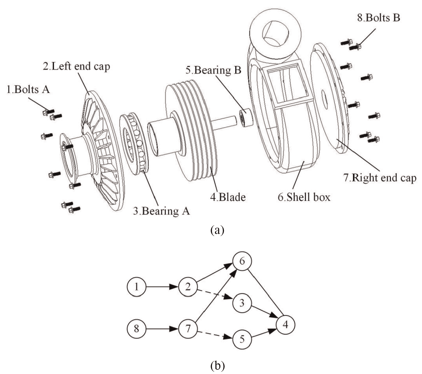
The exploded view and DHGM model of a certain pump: (a) exploded view and (b) the DHGM model.

\begin{matrix} M_{T} = [\begin{matrix} a_{11}^{T} & a_{12}^{T} & \dots & a_{1 n}^{T} \\ a_{21}^{T} & a_{22}^{T} & \dots & a_{2 n}^{T} \\ ⋮ & ⋮ & ⋮ \\ a_{n 1}^{T} & a_{n 2}^{T} & \dots & a_{nn}^{T} \end{matrix}], \\ a_{ij} = {\begin{matrix} 1 if part i and part j are in \\ contact with each other \\ 0 otherwise \end{matrix} \end{matrix}

(1)

\begin{matrix} M_{C} = [\begin{matrix} b_{11}^{C} & b_{12}^{C} & \dots & b_{1 n}^{C} \\ b_{21}^{C} & b_{22}^{C} & \dots & b_{2 n}^{C} \\ ⋮ & ⋮ & ⋮ \\ b_{n 1}^{C} & b_{n 2}^{C} & \dots & b_{nn}^{C} \end{matrix}], \\ b_{ij} = {\begin{matrix} 1 if part i constrain part j \\ 0 otherwise \end{matrix} \end{matrix}

(2)

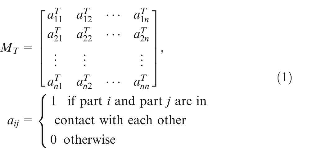
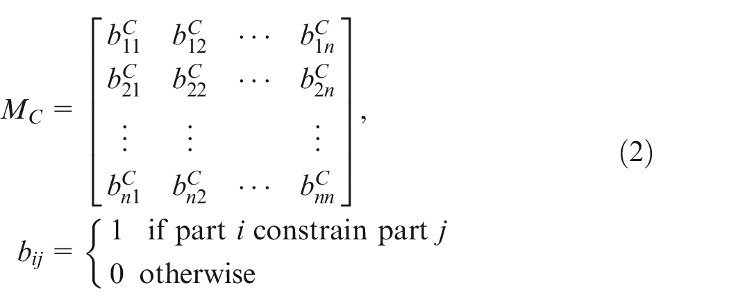
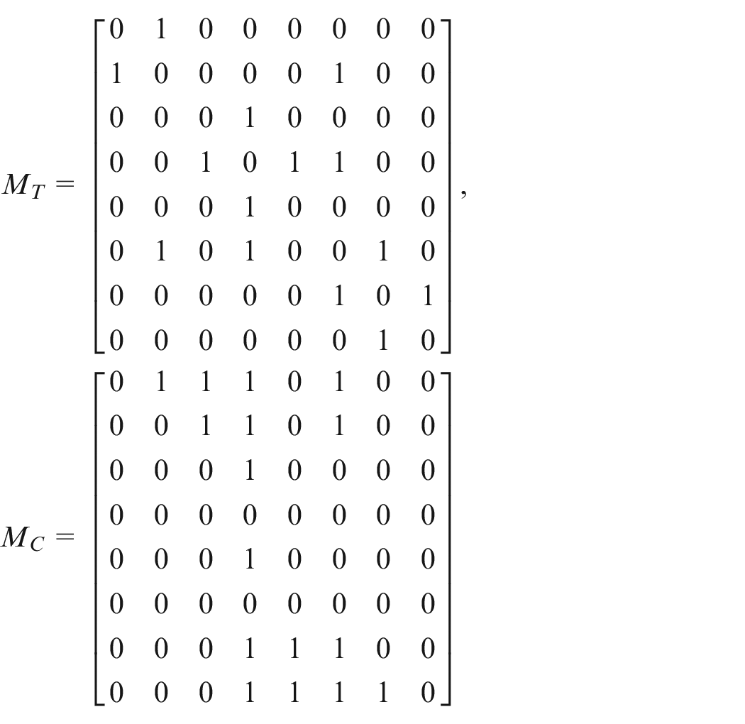
In order to facilitate the subsequent programming, based on DHGM, the contact matrix M_T = (V, E_f) and the constraint matrix M_C = (V, E_fc, E_c) are developed to describe the contact and precedence relationships. Supposing that V contains n parts, the meanings of M_T and M_C’s basic elements are shown in equations (1) and (2), and the M_T and M_c of Figure 1(b) are as follows:

\begin{matrix} M_{T} = [\begin{matrix} 0 & 1 & 0 & 0 & 0 & 0 & 0 & 0 \\ 1 & 0 & 0 & 0 & 0 & 1 & 0 & 0 \\ 0 & 0 & 0 & 1 & 0 & 0 & 0 & 0 \\ 0 & 0 & 1 & 0 & 1 & 1 & 0 & 0 \\ 0 & 0 & 0 & 1 & 0 & 0 & 0 & 0 \\ 0 & 1 & 0 & 1 & 0 & 0 & 1 & 0 \\ 0 & 0 & 0 & 0 & 0 & 1 & 0 & 1 \\ 0 & 0 & 0 & 0 & 0 & 0 & 1 & 0 \end{matrix}], \\ M_{C} = [\begin{matrix} 0 & 1 & 1 & 1 & 0 & 1 & 0 & 0 \\ 0 & 0 & 1 & 1 & 0 & 1 & 0 & 0 \\ 0 & 0 & 0 & 1 & 0 & 0 & 0 & 0 \\ 0 & 0 & 0 & 0 & 0 & 0 & 0 & 0 \\ 0 & 0 & 0 & 1 & 0 & 0 & 0 & 0 \\ 0 & 0 & 0 & 0 & 0 & 0 & 0 & 0 \\ 0 & 0 & 0 & 1 & 1 & 1 & 0 & 0 \\ 0 & 0 & 0 & 1 & 1 & 1 & 1 & 0 \end{matrix}] \end{matrix}

(2)

Notations and assumption

Notations and major assumptions are summarised as follows.

Notations

P: Parts set;

x: Appointed part or target part;

d: Parallel degree, the maximum number of parts can be disassembled in one process;

ap_i: The number of parts can be disassembled in the process i;

n: Total number of parts;

m: The actual number of parts removed;

p: The number of processes till x have been disassembled;

M: Manipulators set;

m_i: Manipulator i, m_i∈M;

PDS: Parallel disassembly sequence, PDS = [PS, SS, MS];

PS: Part sequence, PS = [a_i]_1×n, a_i∈P;

SS: Step-size sequence, SS = [b_i]_1×n, b_i≤d;

MS: Manipulator sequence, MS=[c_i]_1×n, c_i∈M;

tp: Total number of processes for PS;

ej i: part #e, which disassembled by m_j in process i, e_i^j∈P;

BDT(ej i): Basic disassembly time (BDT) operator, BDT of e_i^j;

T(ej i): Tool operator, disassembly tool for e_i^j;

DO(ej i): Direction operator, disassembly direction of e_i^j;

TET: Tool exchange time, it is set to 3S;

DCT: Direction change time, it is set to 2S;

Assumptions

(1): SPDSP is an idealised procedure of non-destructive disassembly procedure that does not damage parts during disassembly;

(2): The manipulator will not break down;

(3): The disassembly time and cost of each part are predetermined and constant;

(4): The manipulators start to work simultaneously in one process;

(5): The part with maximum disassembly time determines the disassembly time of a process.

Parallel disassembly sequence model

The parallel disassembly sequence (PDS) model is introduced in this section. The PDS consists of three segments: part sequence (PS), step-size sequence (SS) and manipulator sequence (MS). Figure 2 illustrates the relationship between the three segments. The corresponding manipulator will disassemble each unit in PS in MS, and each unit in SS means that the number of parts disassembled at the same time of process i. As shown in Figure 2, a_i will be disassembled by c_i, and b_k indicates that b_k parts can be disassembled simultaneously in process k.

Figure 2.

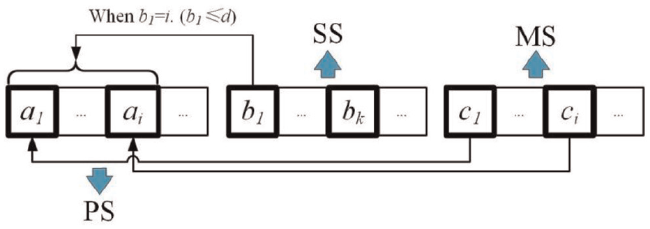
PDS model.

A part can be disassembled if it is unconstrained and in contact with only one part. According to this rule, the parts that can be disassembled in one step can be determined, and the PDS sequence is generated as follows: Scanning M_T and M_C, find all the parts P_i that can be disassembled of the process i. Combining the parallel degree d, select ap_i parts from P_i and fill PS sequentially. Then, set b_i = ap_i and randomly assign ap_i parts to each manipulator.

Solution decoding and evaluation

Extract the fragment involving the target part x, determine each process’s specific task, and solve SPDSP. This procedure is called decoding and is summarised as follows:

Step 1. Find x and the process b_i it belongs to in SS;

Step 2. Assign a_j to the corresponding manipulator till part x.

For example, set PS = [2, 4, 3, 1, 5], SS = [2, 2, 1, 0, 0], MS = [1, 2, 2, 1, 1], d = 2 and x = #3. According to the decoding rule in section Parallel disassembly sequence model, #2 and #4 will be removed by m₁ and m₂, respectively, in the first process. #3 will be disassembled by m₂ in the second process. Due to parts’ constraints, some manipulators will inevitably stay idle in some processes. The quality of the disassembly scheme can be judged based on the fitness function introduced in section 3.

The SPDSP model description

Disassembly time

In terms of disassembly time, three factors need to be considered: total basic disassembly time (TBDT), total tool exchange time (TTET) and total direction change time (TDCT).^7,23 It is more complicated than the SDSP since multiple manipulators perform tasks simultaneously. There are no papers based on this model to study PDSP and SPDSP’s disassembly time, and a modified model will be demonstrated in this section.

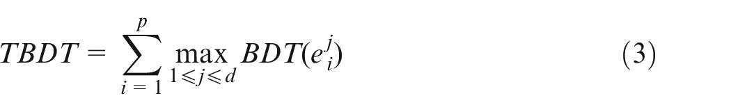
Total basic disassembly time

The basic disassembly time (BDT) of a part is the most necessary time to disassemble a part, and the total BDT (TBDT) can be denoted as follows, where BDT(e_i^j) implies the basic disassembly time of the manipulator j in the process i.

TBDT = \sum_{i = 1}^{p} max_{1 \leq j \leq d} BDT (e_{i}^{j})

(3)

Additional time

It is common to change the disassembly tool at the interval of two adjacent processes, and the tool exchange time (TET) needs to be considered. If one manipulator changes its disassembly tool between two adjacent processes, TET will be considered and total TET (TTET) can be denoted as follows:

Δ_{i} (T (e_{i}^{j}) T (e_{i + 1}^{j})) = {\begin{matrix} 1 T (e_{i}^{j}) \neq T (e_{i + 1}^{j}) \\ 0 T (e_{i}^{j}) = T (e_{i + 1}^{j}) \end{matrix}

(4)

TTET = TET \cdot \sum_{i = 1}^{p - 1} max_{1 \leq j \leq d} Δ_{i} (T (e_{i}^{j}) T (e_{i + 1}^{j}))

(5)

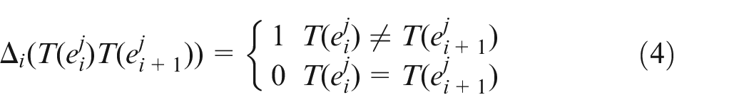
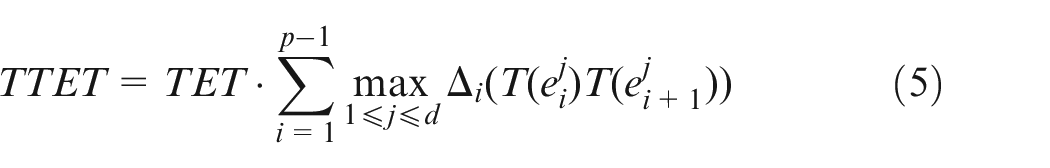
Where Δ_i is the tool exchange operator, T(ej i) is the tool used in the process i by manipulator j for the disassembly of part e.

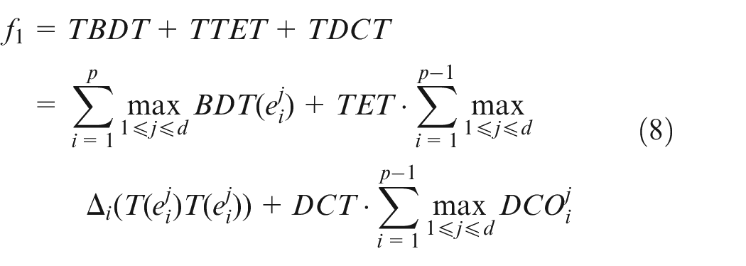
The total direction change time (TDCT) is another essential part of the disassembly time model. Suppose that the direction of each part is represented by the direction operator DO(ej i). If the direction of the two parts is different, the direction compensation operator DCOj i needs to be calculated by equation (6), and the TDCT is denoted as equation (7).

{DCO}_{i}^{j} = \frac{| DO (e_{i}^{j}) - DO (e_{i + 1}^{j}) |}{90 °}

(6)

TDCT = DCT \cdot \sum_{i = 1}^{p - 1} max_{1 \leq j \leq d} {DCO}_{i}^{j}

(7)

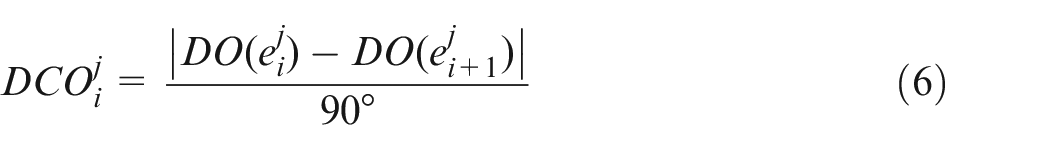
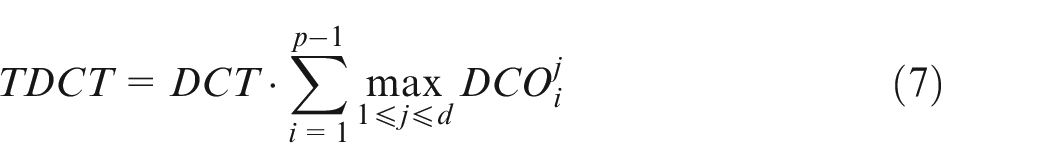
In equations (6) and (7), where DO(ej i) is the direction in which the part is disassembled by manipulator j in the process i; DCOj i is the direction compensation operator used to calculate the changing angle of manipulator j in two adjacent processes. Note that if a manipulator worked at the current process and is idle in the next process, the direction and tool will not be changed, and the total disassembly time is presented in equation (8):

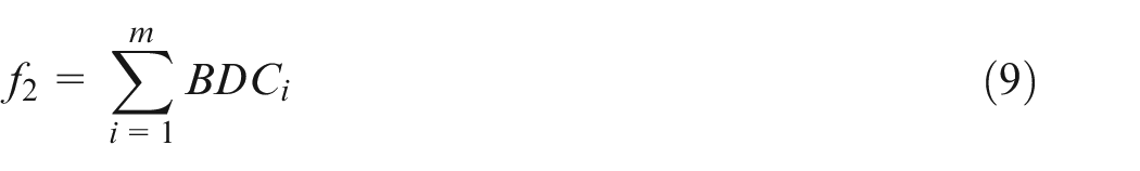
\begin{matrix} f_{1} = TBDT + TTET + TDCT \\ = \sum_{i = 1}^{p} max_{1 \leq j \leq d} BDT (e_{i}^{j}) + TET \cdot \sum_{i = 1}^{p - 1} max_{1 \leq j \leq d} \\ Δ_{i} (T (e_{i}^{j}) T (e_{i}^{j})) + DCT \cdot \sum_{i = 1}^{p - 1} max_{1 \leq j \leq d} {DCO}_{i}^{j} \end{matrix}

(8)

Cost

The basic disassembly cost (BDC) refers to the necessary cost of removing a subassembly, such as dismantling and cleaning. It is assumed that the total cost is related to the parts that have been disassembled. As denoted in equation (9), it is numerically equal to the sum of all parts’ disassembly costs.

f_{2} = \sum_{i = 1}^{m} BD C_{i}

(9)

Multi-objective function

In multiple criteria decision-making problems, the analytic hierarchy process (AHP) is widely used.²⁴ According to the normalisation method using the base value of each indicator proposed by Kopacz et al.,²⁵ the base values are replaced by average disassembly time (ADT) and average disassembly cost (ADC) in this model. Note that ADT and ADC are related to x and d, and they are obtained by simulating a sample group with a certain scale (computing of indicators involving decoding method in section Solution decoding and evaluation). Then, the indicators of the solution can be processed by equation (10) to achieve normalisation.

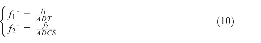
{\begin{matrix} {f_{1}}^{*} = \frac{f_{1}}{ADT} \\ {f_{2}}^{*} = \frac{f_{2}}{ADCS} \end{matrix}

(10)

Finally, the multi-objective function (fitness function) is obtained as follows, and the performance of different solutions can be compared.

min F = \min (w_{1} \cdot {f_{1}}^{*} + w_{2} \cdot {f_{2}}^{*})

(11)

In equation (11), w_i is the weight of indicator i, and w₁+w₂ = 1. According to references on AHP,²⁴w₁ and w₂ are set as 0.667 and 0.333 via scoring and calculating, respectively. A dual-objective disassembly optimisation model is obtained.

The proposed optimisation method

The DSP optimisation has already been proved to be an NP-hard problem. As problem size increases, the solution space will grow exponentially, and metaheuristics are suitable for this scenario because a set of solutions can be processed in parallel, and a similar property might be used for solution recombination. A novel hybrid genetic algorithm (NHGA) is proposed, and its complete procedure is shown in Figure 3, where Ilimit is maximum number of iterations, p_m is mutation possibility, p_c is crossover possibility, Popsize is population size.

Figure 3.

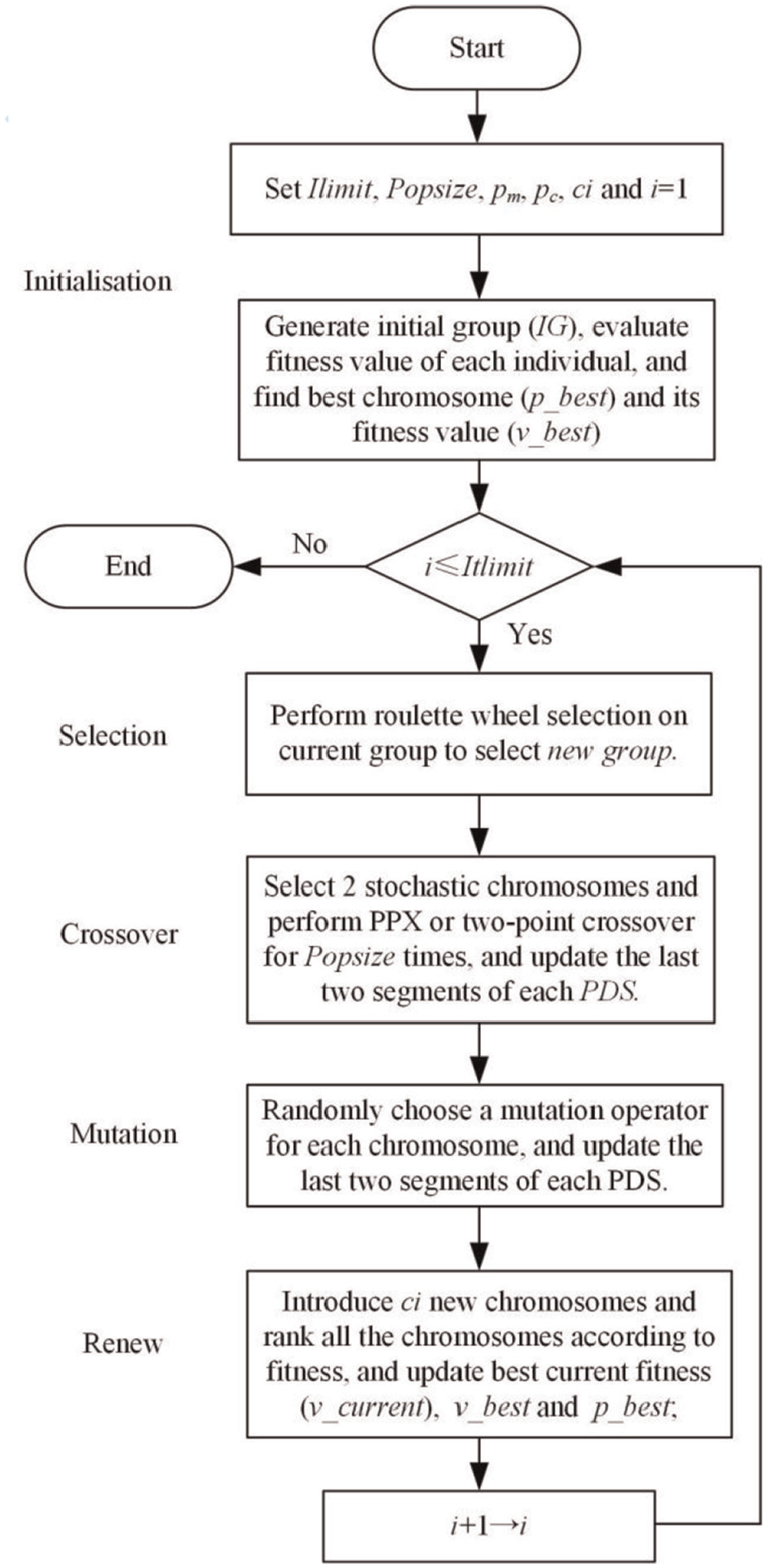
The frame of the optimisation algorithm.

Note that the fitness function, equation (11), is merely used in solution decoding in section Solution decoding and evaluation, and PS is applied to crossover and mutation for solution searching. Once PS changes, MS and SS will be upgraded immediately. Especially for MS, there might be several feasible MS for a PS, which can diversify the population. Then, except for fitness computing, other GA operators are similar with the way treating sequential disassembly sequences. The reciprocal value of the fitness function is applied in Roulette wheel selection for crossover selection.

Crossover

Two kinds of crossover strategies are used, including precedence preservative crossover (PPX) and two-point crossover, and their procedures are shown in Figure 4. Take the PS of the pump model in section 2 as an instance. In PPX, a child mask is a sequence consisting of ‘1’ or ‘2’. ‘1’ and ‘2’ represent the element in the Child that should be taken from which parent chromosome. Taking the child mask [1, 2, 2, 2, 1, 1, 2, 1] in Figure 4(a) to illustrate its mechanism, set the first element of parent 1 to the first element of the Child (part #1), and delete #1 in parent sequence 1 and 2. If the element is zero, fill the Child with the closest non-zero element from left to right and repeat till the child sequence is filled up.

Figure 4.

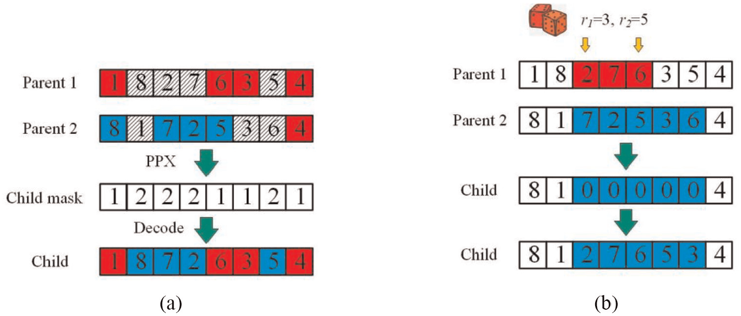
Crossover operators: (a) PPX and (b) two-point crossover.

The other operator is a two-point crossover. Generate two random index points r₁ and r₂, find all the elements that index between r₁ and r₂ in parent 2, and take all the elements between the maximum and minimum index. Finally, reconstruct the Child with sub-sequence according to precedence constraints (see Figure 4(b)). The procedure will be repeated in both operators until the Child is filled and suitable for precedence constraints.

Mutation

Three kinds of neighbour searching methods (namely swap, insert and right point cut operator (RPCO)) is adopted for mutation, and their mechanisms are shown in Figure 5. A PS will randomly choose an operator for mutation.

Figure 5.

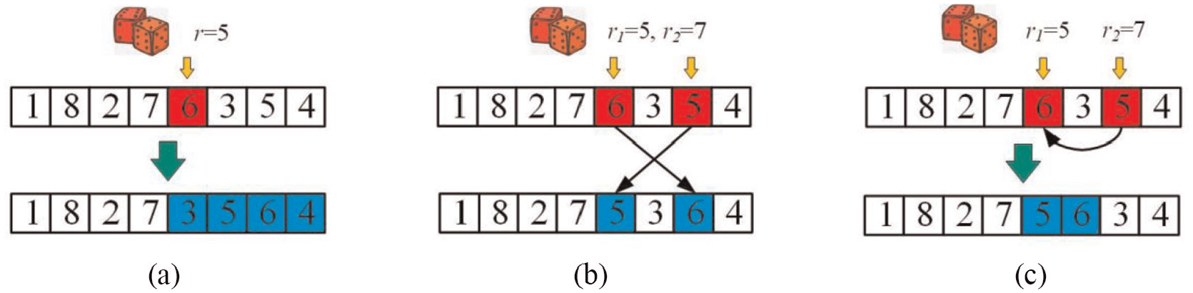
Mutation operator: (a) RPCO, (b) exchange, and (c) swap.

The right point cut operator (RPCO) randomly selects an index and extracts all the subsequent elements. Then, reconstruct the PS from point r to the end with the extracted elements. In the exchange operation, randomly select two points, and exchange them. Swap operation randomly selects a task and inserts it into another random unit. Due to the precedence constraints, the mutation is repeated till a feasible solution is returned.

Renew

The quality of a chromosome might be worse after crossover and mutation. The conventional GA is only confined to the initial population, and it never introduces new individuals except for initialisation. This may lead to converging too fast and reach a locally optimal solution rather than a globally optimal solution. And a new mechanism, renew operator, is introduced, providing more vitality and diversity for searching in the broader space.

The number of new individuals will be determined by comparing the fitness value after crossover and mutation with the current minimum value. Due to the randomness of task assignment, some new chromosomes with better attributes may be obtained. On this basis, a group containing Popsize individuals is selected for the next iteration according to the fitness value; meanwhile, bad chromosomes are eliminated.

Case study and analysis

The proposed methodology is applied in the case of a transmission box shown in Figure 6. The optimisation performance of NHGA and some famous metaheuristic algorithms are compared. All the experiments and simulations are performed on Matlab R2016a.

Figure 6.

The exploded view of the transmission box.

The main parameters in the case are the appointed target part x and parallel degree d, and they can exert great influence in determining the scale and values of the solutions. For the control parameters of NHGA, set the maximum iteration time Ilimit = 300, the population size PopSize = 50, the crossover possibility p_c = 0.8 and the mutation possibility p_m = 0.3.

Case study

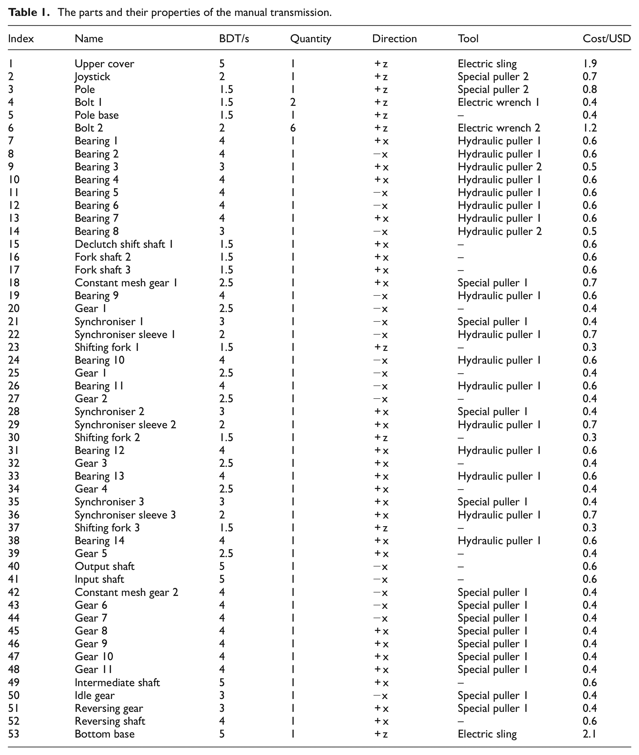
The product’s DHGM is presented in Figure 7, M_T and M_C are in Appendix Figures A1 and A2. The attributes of all the parts and disassembly tools are shown in Table 1. For simplification, the same parts are considered as one part, and it is assumed that the bottom base and its internal parts can be removed after all upper parts have been completely removed.

Table 1.

The parts and their properties of the manual transmission.

Index	Name	BDT/s	Quantity	Direction	Tool	Cost/USD
1	Upper cover	5	1	+z	Electric sling	1.9
2	Joystick	2	1	+z	Special puller 2	0.7
3	Pole	1.5	1	+z	Special puller 2	0.8
4	Bolt 1	1.5	2	+z	Electric wrench 1	0.4
5	Pole base	1.5	1	+z	–	0.4
6	Bolt 2	2	6	+z	Electric wrench 2	1.2
7	Bearing 1	4	1	+x	Hydraulic puller 1	0.6
8	Bearing 2	4	1	−x	Hydraulic puller 1	0.6
9	Bearing 3	3	1	+x	Hydraulic puller 2	0.5
10	Bearing 4	4	1	+x	Hydraulic puller 1	0.6
11	Bearing 5	4	1	−x	Hydraulic puller 1	0.6
12	Bearing 6	4	1	−x	Hydraulic puller 1	0.6
13	Bearing 7	4	1	+x	Hydraulic puller 1	0.6
14	Bearing 8	3	1	−x	Hydraulic puller 2	0.5
15	Declutch shift shaft 1	1.5	1	+x	–	0.6
16	Fork shaft 2	1.5	1	+x	–	0.6
17	Fork shaft 3	1.5	1	+x	–	0.6
18	Constant mesh gear 1	2.5	1	+x	Special puller 1	0.7
19	Bearing 9	4	1	−x	Hydraulic puller 1	0.6
20	Gear 1	2.5	1	−x	–	0.4
21	Synchroniser 1	3	1	−x	Special puller 1	0.4
22	Synchroniser sleeve 1	2	1	−x	Hydraulic puller 1	0.7
23	Shifting fork 1	1.5	1	+z	–	0.3
24	Bearing 10	4	1	−x	Hydraulic puller 1	0.6
25	Gear 1	2.5	1	−x	–	0.4
26	Bearing 11	4	1	−x	Hydraulic puller 1	0.6
27	Gear 2	2.5	1	−x	–	0.4
28	Synchroniser 2	3	1	+x	Special puller 1	0.4
29	Synchroniser sleeve 2	2	1	+x	Hydraulic puller 1	0.7
30	Shifting fork 2	1.5	1	+z	–	0.3
31	Bearing 12	4	1	+x	Hydraulic puller 1	0.6
32	Gear 3	2.5	1	+x	–	0.4
33	Bearing 13	4	1	+x	Hydraulic puller 1	0.6
34	Gear 4	2.5	1	+x	–	0.4
35	Synchroniser 3	3	1	+x	Special puller 1	0.4
36	Synchroniser sleeve 3	2	1	+x	Hydraulic puller 1	0.7
37	Shifting fork 3	1.5	1	+z	–	0.3
38	Bearing 14	4	1	+x	Hydraulic puller 1	0.6
39	Gear 5	2.5	1	+x	–	0.4
40	Output shaft	5	1	−x	–	0.6
41	Input shaft	5	1	−x	–	0.6
42	Constant mesh gear 2	4	1	−x	Special puller 1	0.4
43	Gear 6	4	1	−x	Special puller 1	0.4
44	Gear 7	4	1	−x	Special puller 1	0.4
45	Gear 8	4	1	+x	Special puller 1	0.4
46	Gear 9	4	1	+x	Special puller 1	0.4
47	Gear 10	4	1	+x	Special puller 1	0.4
48	Gear 11	4	1	+x	Special puller 1	0.4
49	Intermediate shaft	5	1	+x	–	0.6
50	Idle gear	3	1	−x	Special puller 1	0.4
51	Reversing gear	3	1	+x	Special puller 1	0.4
52	Reversing shaft	4	1	+x	–	0.6
53	Bottom base	5	1	+z	Electric sling	2.1

Figure 7.

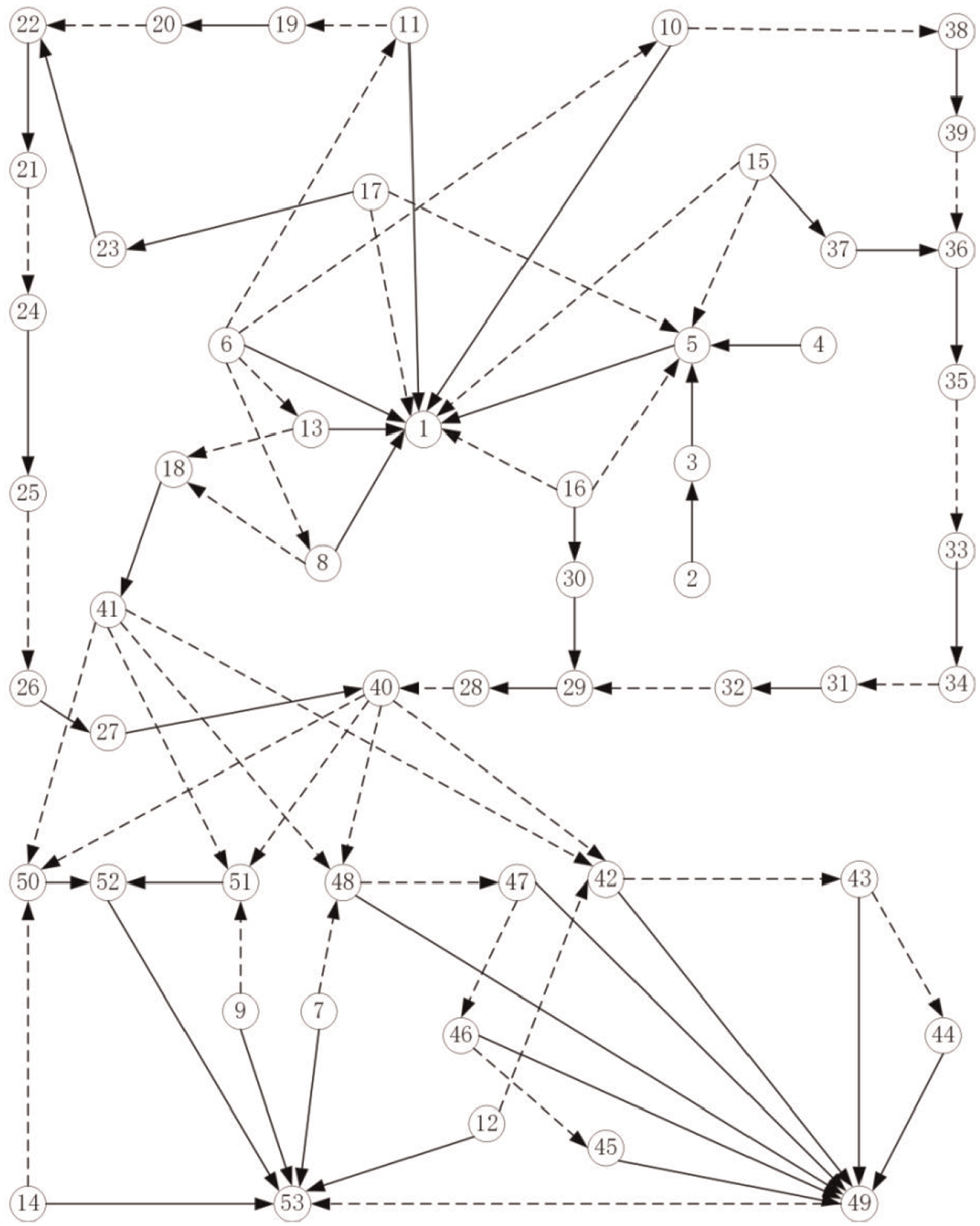
DHGM of the instance.

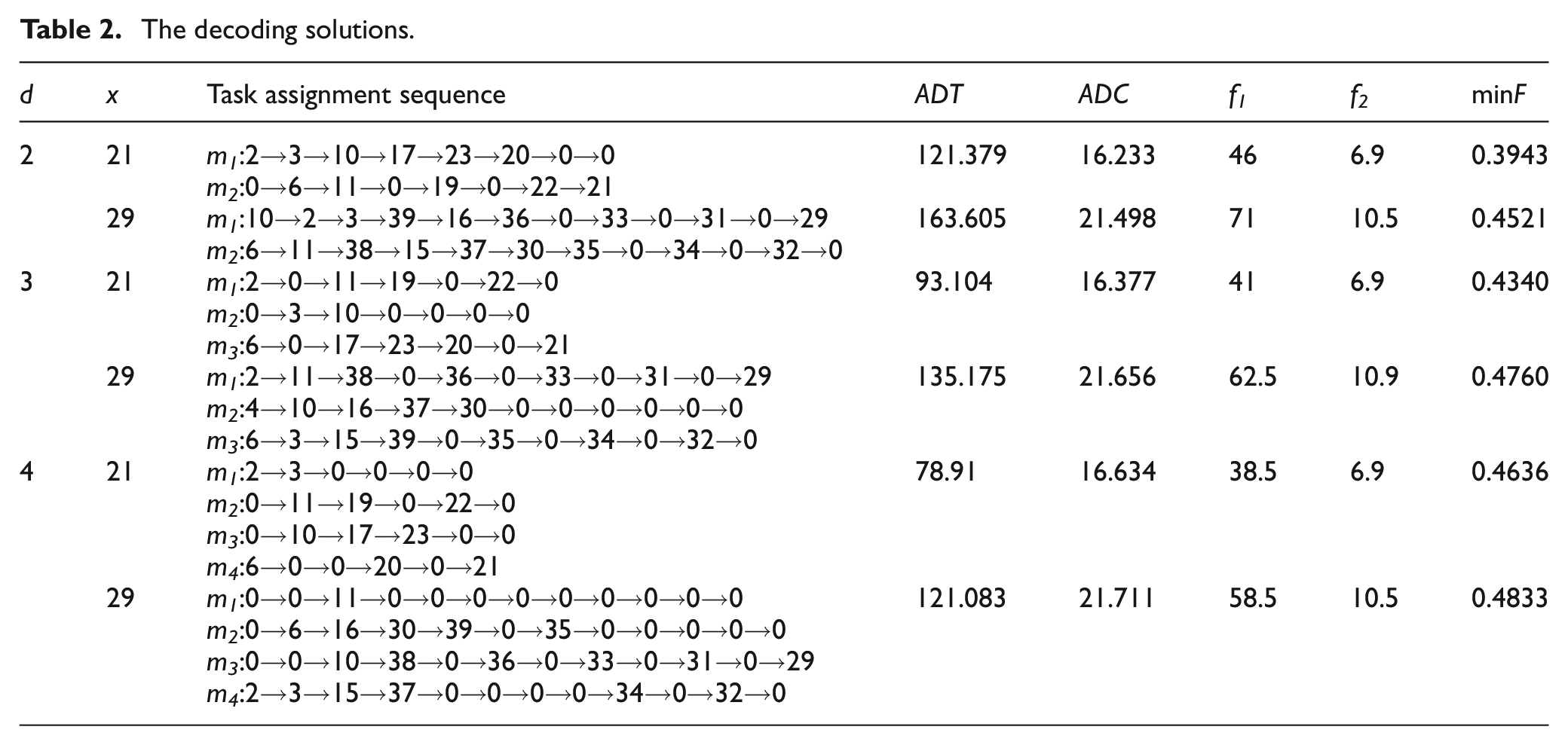
d is set to 2, 3, 4, and x is appointed as 21 and 29, and the results and optimisation performance are shown in Table 2 and Figure 8, where m_i represent manipulator i. The sixth and seventh columns show the value of disassembly time and cost. It is a pity that the BDT and cost are not using actual data, and they are determined on simulation, and the feasibility of the methodology will not be affected. ADT and ADC are obtained by simulation, as shown in the fourth and fifth columns in Table 2, respectively.

Table 2.

The decoding solutions.

d	x	Task assignment sequence	ADT	ADC	f₁	f₂	minF
2	21	m₁:2→3→10→17→23→20→0→0	121.379	16.233	46	6.9	0.3943
	21	m₂:0→6→11→0→19→0→22→21	121.379	16.233	46	6.9	0.3943
	29	m₁:10→2→3→39→16→36→0→33→0→31→0→29	163.605	21.498	71	10.5	0.4521
	29	m₂:6→11→38→15→37→30→35→0→34→0→32→0	163.605	21.498	71	10.5	0.4521
3	21	m₁:2→0→11→19→0→22→0	93.104	16.377	41	6.9	0.4340
		m₂:0→3→10→0→0→0→0
		m₃:6→0→17→23→20→0→21
	29	m₁:2→11→38→0→36→0→33→0→31→0→29	135.175	21.656	62.5	10.9	0.4760
		m₂:4→10→16→37→30→0→0→0→0→0→0
		m₃:6→3→15→39→0→35→0→34→0→32→0
4	21	m₁:2→3→0→0→0→0	78.91	16.634	38.5	6.9	0.4636
		m₂:0→11→19→0→22→0
		m₃:0→10→17→23→0→0
		m₄:6→0→0→20→0→21
	29	m₁:0→0→11→0→0→0→0→0→0→0→0→0	121.083	21.711	58.5	10.5	0.4833
		m₂:0→6→16→30→39→0→35→0→0→0→0→0
		m₃:0→0→10→38→0→36→0→33→0→31→0→29
		m₄:2→3→15→37→0→0→0→0→34→0→32→0

Figure 8.

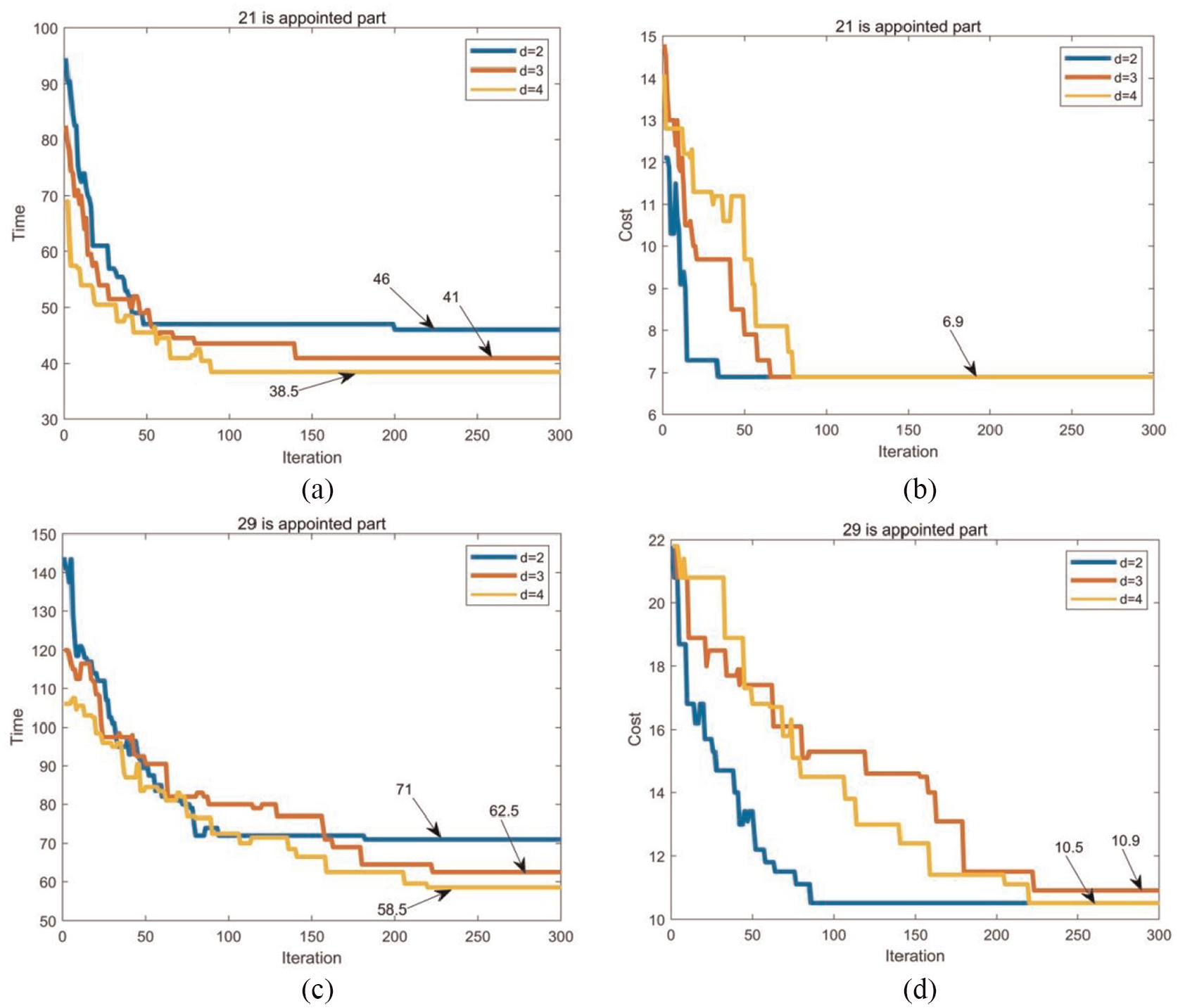
Time and cost of NHGA: (a) result of disassembly time of part #21, (b) result of disassembly cost of part #21, (c) result of disassembly time of part #29, and (d) result of disassembly cost of part #29.

From the analysis of (b) and (d) in Figure 8, once x is determined, the number and type of parts are also determined after iteration. For instance, in (b), although d is different, after the iteration, the final cost also converges to 6.9; in Figure 8(d), d = 2 and 4 also converge to 10.5. But for disassembly time, it will be different. Due to multiple manipulators, the efficiency is improved compared with sequential disassembly. However, if the total disassembly process is not complicated, for example, x = 21, there is no significant improvement in disassembly efficiency. Moreover, several manipulators will stay idle, as shown in Table 2 (d = 4, x = 29). In this case, the additional process is the most critical factor affecting disassembly efficiency, and it is not advisable to increase manipulators to improve disassembly efficiency.

Comparison with other methods

To test the performance of the proposed method, the computational results are compared with conventional GA,²³ simulated annealing (SA)²⁶ and tabu search (TS).²⁷ The number of iterations of SA and TS is Ilimit × group_size, and the best solutions in each group_size times will be compared with the result obtained in each generation of NHGA. The same sequence model, decoding methods (see section 2), and objective functions are used. The results are shown in Figure 9 and Table 3. In Figure 9, (a), (b), and (c) show the result of #21 part with different d; (d), (e) and (f) show the result of #29 part with different d.

Table 3.

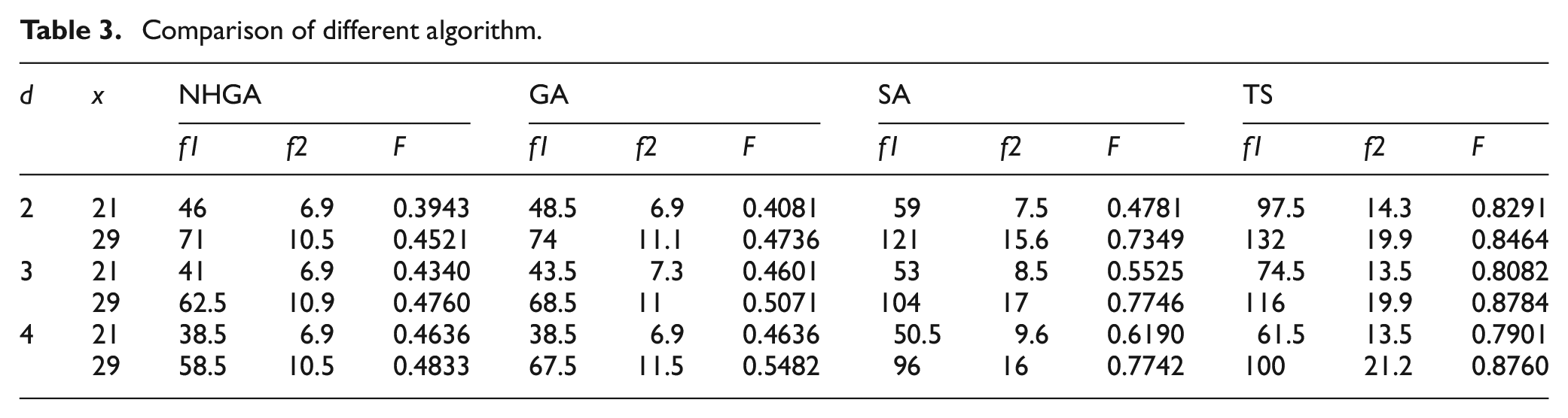
Comparison of different algorithm.

d	x	NHGA			GA			SA			TS
		f1	f2	F	f1	f2	F	f1	f2	F	f1	f2	F
2	21	46	6.9	0.3943	48.5	6.9	0.4081	59	7.5	0.4781	97.5	14.3	0.8291
2	29	71	10.5	0.4521	74	11.1	0.4736	121	15.6	0.7349	132	19.9	0.8464
3	21	41	6.9	0.4340	43.5	7.3	0.4601	53	8.5	0.5525	74.5	13.5	0.8082
3	29	62.5	10.9	0.4760	68.5	11	0.5071	104	17	0.7746	116	19.9	0.8784
4	21	38.5	6.9	0.4636	38.5	6.9	0.4636	50.5	9.6	0.6190	61.5	13.5	0.7901
4	29	58.5	10.5	0.4833	67.5	11.5	0.5482	96	16	0.7742	100	21.2	0.8760

Figure 9.

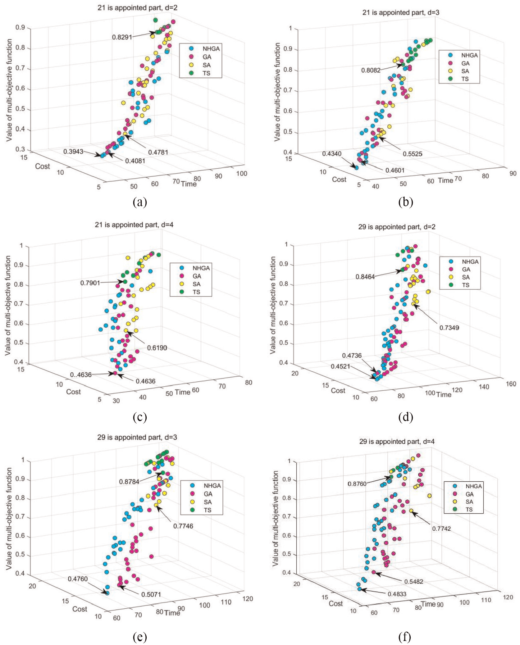
The result of multi-objective optimisation: (a) d = 2, part #21, (b) d = 3, part #21, (c) d = 4, part #21, (d) d = 2, part #29, (e) d = 3, part #29, and (f) d = 4, part #29.

The results of these six experiments were iterated for Ilimit times, and the results in Figure 9 consist of disassembly time, cost and value of normalised multi-objection function. Take #29 part as an example, combined with Figure 9 and Table 3, when d = 2, the values of disassembly time are 71, 74, 121 and 132 s of NHGA, GA, SA and TS, respectively. Meanwhile, it can also be seen that NHGA has the best performance and a similar performance in other scenarios, especially for x, which has a long task assignment sequence and complicated structure. In addition, combined with computational results in Table 3, TS has the worst performance, and SA is the second-worst method. The performance of the algorithms can be ranked as follows: NHGA > GA > SA > TS.

Conclusion and future work

In this paper, a novel selective parallel disassembly methodology is proposed. Firstly, a graph model, contact matrix M_T and precedence matrix M_C are used to quantify the priority relationship for disassembly. Secondly, a PDS model and a decoding method for SPDSP are designed. With the support of M_T and M_C, an algorithm for PDS generation is discussed. Thirdly, a method for decoding PDS into task assignment sequence for indicators’ computation method is developed to minimise the disassembly time and cost. Finally, the GA’s crossover and mutation operators are modified and applied to the multi-objective optimisation process. A manual transmission box was selected as an instance to demonstrate the correctness of the methodology. The parallel degree d and target part x were set to different values. The line charts of the time and cost objective functions show the disassembly efficiency of different d. The two objectives are integrated into the fitness function by AHP, and scatter plots in Figure 9 illustrate different algorithms’ optimisation performance. In addition, the additional time is applied to parallel disassembly in this study, and the optimisation method achieves the effect, shortening the disassembly time and reducing the cost.

But there are still some limitations. Firstly, in terms of data, such as disassembly time and cost, we just made an estimation and did not use the actual disassembly data. Secondly, the methodology is based on the assumption that all the manipulators start disassembly at the same time in a process, and it is a synchronised disassembly activity. Although the efficiency is greatly improved compared with sequential disassembly, idle time still exists, causing unnecessary waste of time. All of these need to be studied in the future.

Footnotes

Appendix

Declaration of conflicting interests

The author(s) declared no potential conflicts of interest with respect to the research, authorship, and/or publication of this article.

Funding

The author(s) disclosed receipt of the following financial support for the research, authorship, and/or publication of this article: This research was supported by the National Nature Science Foundation of China [grant number 51875156] and the 2018 Open Research Fund by Jiangsu Key Laboratory of Recycling and Reuse Technology for Mechanical and Electronic Products [grant number RRME 201803].

ORCID iD

Lei Zhang

References

Zhou

Liu

Pham

, et al. Disassembly sequence planning: recent developments and future trends. Proc IMechE, Part B: J Engineering Manufacture 2019; 233(5): 1450–1471.

Seitz

. A critical assessment of motives for product recovery: the case of engine remanufacturing. J Clean Prod 2007; 15(11–12): 1147–1157.

Huang

Pham

Wang

, et al. A case study in human-robot collaboration in the disassembly of press-fitted components. Proc IMechE, Part B: J Engineering Manufacture 2020; 234(3): 654–664.

Tian

Zhou

. Disassembly sequence planning considering fuzzy component quality and varying operational cost. IEEE Trans Autom Sci Eng 2018; 15(2): 748–760.

Smith

Hung

. A novel selective parallel disassembly planning method for green design. J Eng Des 2015; 26(10–12): 283–301.

Ren

Zhang

Zhao

, et al. An asynchronous parallel disassembly planning based on genetic algorithm. Eur J Oper Res 2018; 269(2): 647–660.

Wahab

Rahman

MNA

, et al. Genetically optimised disassembly sequence for automotive component reuse. Expert Syst Appl 2012; 39(5): 5409–5417.

Ren

Meng

Zhang

, et al. An efficient metaheuristics for a sequence-dependent disassembly planning. J Clean Prod 2020; 245: 118644.

Huang

Fuh

JYH

, et al. A multi-objective disassembly planning approach with ant colony optimization algorithm. Proc IMechE, Part B: J Engineering Manufacture 2008; 222(11): 1465–1474.

10.

Zhang

Liu

Qiu

, et al. Disassembly sequence planning using a fast and effective precedence-based disassembly subset-generation method. Proc IMechE, Part B: J Engineering Manufacture 2019; 234(3): 513–526.

11.

Zhang

Zhao

, et al. Disassembly line balancing optimization method for high efficiency and low carbon emission. Int J Precis Eng Manuf Green Technol 2019; 8(1): 233–247.

12.

Kheder

Trigui

Aifaoui

. Disassembly sequence planning based on a genetic algorithm. Proc IMechE, Part C: J Mechanical Engineering Science 2014; 229(12): 2281–2290.

13.

Smith

Hsu

Smith

. Partial disassembly sequence planning based on cost-benefit analysis. J Clean Prod 2016; 139: 729–739.

14.

Tian

Ren

Feng

, et al. Modeling and planning for dual-objective selective disassembly using AND/OR graph and discrete artificial bee colony. IEEE Trans Ind Inf 2019; 15(4): 2456–2468.

15.

Ren

Tian

Zhao

, et al. Selective cooperative disassembly planning based on multi-objective discrete artificial bee colony algorithm. Eng Appl Artif Intell 2017; 64: 415–431.

16.

Jin

Wang

, et al. A systematic selective disassembly approach for Waste Electrical and Electronic Equipment with case study on liquid crystal display televisions. Proc IMechE, Part B: J Engineering Manufacture 2017; 231(13): 2261–2278.

17.

Zhu

Sarigecili

Roy

. Disassembly information model incorporating dynamic capabilities for disassembly sequence generation. Robot Comput Integr Manuf 2013; 29(5): 396–409.

18.

Ullerich

Buscher

. Flexible disassembly planning considering product conditions. Int J Prod Res 2013; 51(20): 6209–6228.

19.

Srinivasan

Gadh

. A geometric algorithm for single selective disassembly using the wave propagation abstraction. Comput Aided Des 1998; 30(8): 603–613.

20.

Kara

Pornprasitpol

Kaebernick

. A selective disassembly methodology for end-of-life products. Assem Autom 2005; 25(2): 124–134.

21.

Berg

Behdad

Vance

, et al. Disassembly sequence evaluation: a user study leveraging immersive computing technologies. J Comput Inf Sci Eng 2015; 15(1): 7.

22.

Zhang

, et al. Parallel disassembly sequence planning for complex products based on fuzzy-rough sets. Int J Adv Manuf Technol 2014; 72 (1–4): 231–239.

23.

Kongar

Gupta

. Disassembly sequencing using genetic algorithm. Int J Adv Manuf Technol 2006; 30 (5–6): 497–506.

24.

Saaty

. Scaling method for priorities in hierarchical structures. J Math Psychol 1977; 15(3): 234–281.

25.

Kopacz

Kryzia

. Assessment of sustainable development of hard coal mining industry in Poland with use of bootstrap sampling and copula-based Monte Carlo simulation. J Clean Prod 2017; 159: 359–373.

26.

Kalayci

Gupta

. Balancing a sequence-dependent disassembly line using simulated annealing algorithm. Appl Manage Sci 2013; 16: 81–103.

27.

Kalayci

Gupta

. A tabu search algorithm for balancing a sequence-dependent disassembly line. Prod Plan Control 2013; 25(2): 149–160.

A systematic approach in remanufacturing for high efficiency and low cost: The selective parallel disassembly sequence planning

Abstract

Keywords

Introduction

Notation and sequence model

Disassembly information model

Notations and assumption

Notations

Assumptions

Parallel disassembly sequence model

Solution decoding and evaluation

The SPDSP model description

Disassembly time

Total basic disassembly time

Additional time

Cost

Multi-objective function

The proposed optimisation method

Crossover

Mutation

Renew

Case study and analysis

Case study

Comparison with other methods

Conclusion and future work

Footnotes

Appendix

Declaration of conflicting interests

Funding

ORCID iD

References