Variation propagation modeling and pattern mapping method for aircraft assembly structure considering residual stress from manufacturing process

Abstract

Bulk residual stress of component originating from material preparation processing has an impact on large-scale assembly deformation and consequently affects dimensional and shape accuracy of assembly especially for those thick and asymmetric components. This article proposes a quantitative variation propagation modeling method, highlighting the subsequent impact of initial residual stress in raw material, and provides an effective pattern mapping method between bulk stress fluctuation and overall component or assembly deformation. The basic analysis approach considering residual stress is validated by test experiments previously. Legendre polynomials and Spline functions are employed to represent stress perturbation pattern and localized deformation pattern, respectively. Variation propagation is modeled in a case study of the horizontal stabilizer assembly system based on these non-linear mathematical representations. The orthogonal test is designed utilizing finite element analysis to simulate principal stress component perturbation. Corresponding regression analysis aimed at the optimized geometric target is conducted leading to confined Legendre coefficients range for better match. The mapping relation is developed graphically between Legendre coefficient’s pattern and Spline coefficient’s pattern revealing the region of influence and offers assembly deformation prediction as well as practical component selection suggestion for better match. The downstream quality control can be further traced back to the parameter setting of material preparation processing like stretch ratio. The methods we present help systematically improving compliant assembly precision in consideration with residual stress factor in aircraft assembly structure.

Introduction

It is widely accepted that residual stress has significant influence on the distortion of engineering component. Initial bulk residual stress exists inevitably in the raw material. After machining, when some of bulk stress is released by material removal, component deformation occurs; under certain conditions, usually for those work pieces with considerable thickness, material bulk residual stress dominates distortion compared with machining-induced residual stress.^1–4 During the subsequent assembling process of compliant components, internal stress redistribution coupled with the residual stress resulting from fabrication history takes place in the spring-back after releasing the clamps. This causes new assembly’s dimensional variation and affects its shape accuracy.

Aircraft assemblies like horizontal stabilizer and wing box can be viewed as a frame structure covered by skin panels. The frame is composed of main supporting components, such as edges, spars and beams. These thick components combined with comparatively thinner ribs or webs offer a basic overall shape of structure. The initial bulk stress in materials is the major original source of large-scale integral warping for the thick components themselves and for the following important frame structure as well. The corresponding aerodynamic configuration requirements need to be satisfied after further joining the skin panels. It is the fundamental prerequisite that the assembly quality of the frame itself should be guaranteed in the first place.

Previous studies in civil aircraft assembly field focused on the joining aspects of thin-walled parts. Saadat et al.^5–7 proposed an effective prediction system which modeled the geometrical variation propagation caused by sequent joining for the assembly of rib feet and skin panels of an Airbus wing-box structure using finite element method (FEM) and it helped to implement corrective actions like adjusting the rib or pre-drilling the holes on each rib foot for better match. Cheng and colleagues^8,9 established a variation propagation model for a multi-state riveting process of a wing panel which was made up of skin and stringers, and the setup planning approach was proposed to accomplish riveting work by minimum variation. In the general research area of compliant assembly variation analysis, Hu and Koren ¹⁰ proposed the “Stream-of-Variation Theory (SoV).” He analyzed the variability for both serial and parallel assembly due to the evolution of the stiffness of assembly structure. State space modeling was applied to the SoV methodology to link the key product characteristics (KPC) with key control characteristics (KCC). ¹¹ Camelio et al. ¹² extended this approach to model the product variation in multi-station assembly systems. The state matrix they formulated concerning deformation and spring-back involved sensitivity matrix which reflected geometrical relation between incoming part variation and output assembly variation. The sensitivity matrix could be obtained through method of influence coefficients (MICs) using FEM. ¹³ The SoV approach was also applied to modeling variation propagation in multi-station machining processes (MMPs). ¹¹ The effect of datum error and fixture error could be obtained by a kinematics analysis based on machined product and process design information. More complicated contributors of machine errors, like spindle thermal–induced variations and cutting-tool wear–induced variations, were incorporated in the conventional SoV model to improve the accuracy of prediction. ¹⁴

However, the above variation propagation modeling ways have not dealt with initial residual stress in raw material as original affecting factor explicitly and quantitatively; thus, they are not quite suitable for the frame assembly. This is a typical case that variation propagation concerning compliant deformation emphasizes the part variation from material preparation, component machining, to multi-station assembly according to the changes of the structure’s features.

The assembly geometric requirement for aerospace product usually holds for overall situation to satisfy functional requirement like skin panel’s aerodynamic shape. The area of frame assembly remained for joining with skin panel requires overall smooth and good flatness to avoid stress concentration since no shims are allowed to use. Therefore, in this case, the assembly deformation of edges which comprise the frame structure mainly should be evaluated through some indicators which can effectively reflect the overall situation.

Additionally, bulk stress fields distribute in the entire material billet. It is insufficient to discover the resultant deformation pattern by inspecting very few individual points along the edges. The component deformation pattern depends on the initial bulk stress distribution in edge’s raw material and the specific geometric characteristics of edge component. The subsequent assembly deformation patterns change with the assembly structures taking edge’s non-ideal geometry and its corresponding stress state as input. It is necessary to figure out the deformation pattern and its transition which reflects the overall situation concisely to enhance the understanding of variation propagation induced by initial bulk residual stress in raw materials.

Variation modes or deformation patterns are often extracted from deviation data. For example, principal component analysis (PCA) is a widely used technique to reduce the dimensionality of highly correlated data via orthogonal projection into a space defined by a few significant eigenvectors. ¹⁵ It was applied to fixture fault diagnosis and identifying sources of dimensional variation in automotive body assembly.^16–18 Wang and Ding ¹⁹ proposed a method to identify sources of variation in horizontal stabilizer assembly of civil aircraft using finite element analysis (FEA) and PCA. The dependence in deviation among the adjacent points was called geometric covariance by Merkley. ²⁰ It arises from surface continuity. The effect of geometric covariance in sheet metal parts implies that different sources of variation over the same surface are highly correlated. Camelio et al. ²¹ took advantage of this effect and used variation vectors defined for each deformation pattern identified from the covariance of the components via PCA. FEA was then used to determine the effect of each deformation pattern over the assembly variation. PCA helps modeling the covariance structure of variation data statistically. To express the relation among the numerous points on the same surface more fully than PCA, shape deviation modeling can be realized from a computational geometry point of view. Merkley ²⁰ proposed to use bounded random Bezier curves to define the statistical gap between mating curves of assembly. Shape deviations were parameterized by constraining the displacement of the control points of Bezier curves. Stout ²² continued Merkley’s research and fitted the surface profiles of the parts with polynomial to compute the covariance. Franciosa et al. ²³ simulated variational shape of parts based on morphing mesh approach as input to variational assembly analysis. The displacement of any mesh node was calculated as a weighted mean of all control points through a predefined polynomial function with influence distance as variable. Control points were randomly generated using a Monte Carlo simulation.

To reflect the overall situation as comprehensive as possible in view of current frame assembly’s structural characteristics, there remains a need for representing not only exact deviation values for numerous points along edges but also their geometric covariance in a compact way.

In this article, we present a variation propagation modeling method, especially for those cases of which bulk residual stress in the material is dominant impact variable responsible for large-scale deformation in subsequent machining and assembly processes; then, an effective pattern mapping method based on the model is proposed for better match of the main thick edges in frame structures.

The article is organized of the following logical structure as shown in Figure 1. First, the basic analysis approach for introducing residual stress factor into assembly variation model is presented with experimental validation. The assembly of horizontal stabilizer is described and some field measuring results are prepared for further processing. Second, Legendre polynomials combination and Spline functions fitting are used as mathematical tools to represent the bulk stress fluctuation and the overall deformation pattern, respectively, and the representations reflecting the variation propagation are illustrated for main edges preliminarily. Third, the orthogonal test is designed via stress component perturbation utilizing FEA simulation, and the corresponding regression analysis is conducted based on the comprehensive evaluation target which leads to confined Legendre coefficients range for better match. Finally, the mapping relation between Legendre coefficients and Spline coefficients is developed graphically revealing the influence regions, the assembly deformation prediction is obtained by transforming Spline coefficients distribution pattern and the corresponding component deformation selection offers practical suggestion for better match.

Figure 1.

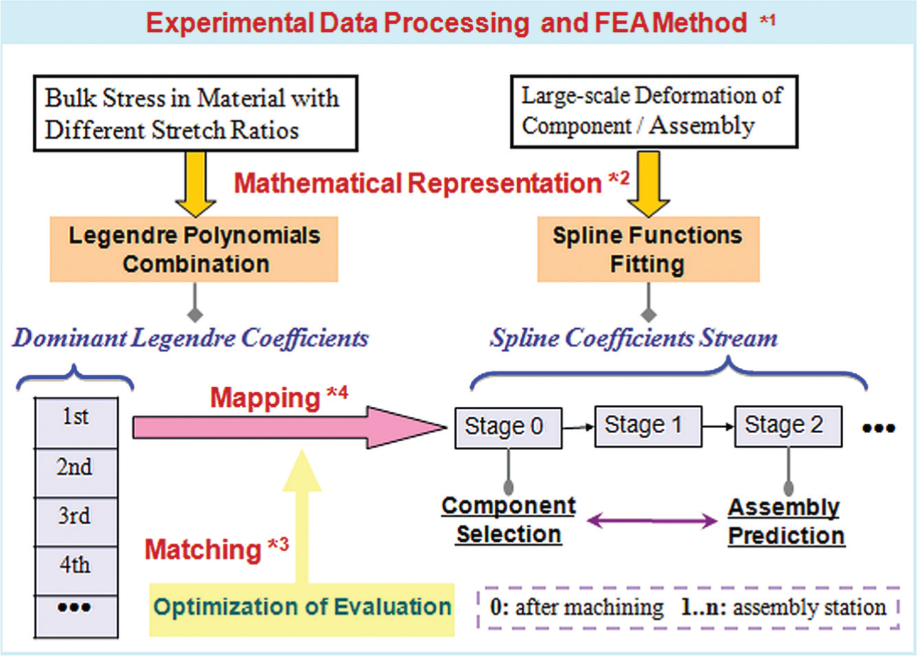
Logical structure of research work.

Basic analysis approach

Estimation of bulk residual stress in material

The estimated quantification of initial residual stress in the material of main edge is based on normalized residual stress shapes of quenched and pre-stretched aluminum alloy thick plates. The normalized stress profiles have “W” or parabolic shapes as we used in our previous study. ²⁴ These stress profiles in the rolling and transverse directions are obtained through statistical methods from numerical results which involve simulated plates with various thicknesses, quenching speeds and stretch ratios in different combinations.^25–27 Normalization is applied to plate’s thickness value on the X-axis and stress value on the Y-axis to get the basic shapes of the profiles which are almost symmetric about the mid-plane. In addition, the regression relation between the actual surface residual stress and key internal peak stress value can be used as empirical formula from the published findings.^25–27

The potential practical stress distribution of edge’s material can be obtained by extending and translating the normalized stress profiles. The corresponding extension ratio and translating amplitude can be calculated proportionally in comparison with the normalized residual stress profiles based on regression relation involving practical surface residual stress measurement. Both extension and translation are linear transformation, thus do not alter the non-linear pattern of stress distribution along the thickness. This non-destructive surface measurement combined with domain knowledge facilitates the estimation of bulk residual stress, and in the meantime saves the raw materials.

Numerical implementation and experimental validation

The finite element (FE) model is created using commercial software ABAQUS CAE as the pre-processor and FEA is carried out using the general-purpose FEA package ABAQUS Standard. The initial bulk residual stress is added to the edge’s raw material using ABAQUS SIGINI Subroutine and FORTRAN programming. After simulating the material removal, the edge component with the corresponding geometric and stress states can be incorporated into the subsequent assembly variation model. The whole procedure was validated through a test structure on the constructed fixture setup shown in Figure 2. Two thick edges and one thin web constituted a typical wedge structure. The surface residual stress states of the edges’ materials were measured using the PROTO iXRD X-ray-diffraction stress measuring system. And FARO Edge was chosen as the shape measuring instrument for the machined test articles and the assembled test structure. Figure 2 shows the assembly state ready to be measured after the clamps are released. Through the modeling method validation and decoupling method validation conducted in our earlier research, the simulations with the introduced residual stress factor improved the accuracy of prediction closer to the results of experimental measurement. ²⁴

Figure 2.

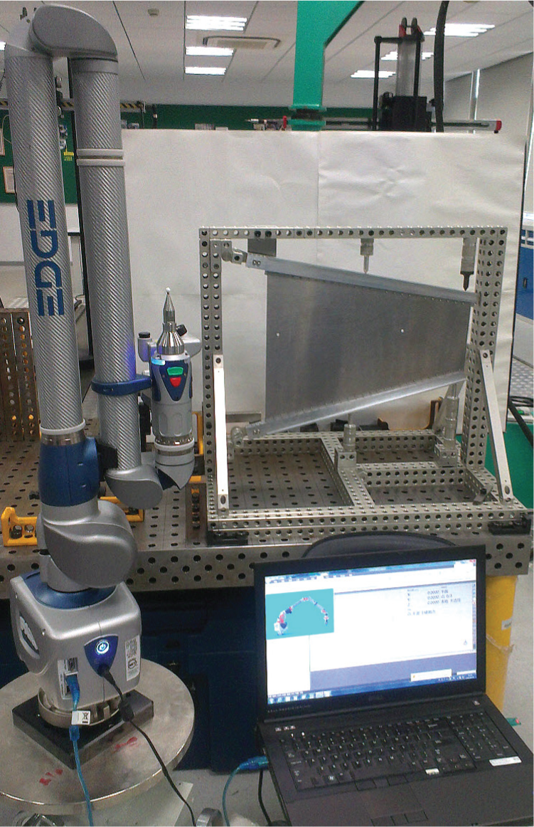
Overall view of the assembly experimental implementation.

Source of error and uncertainty

The greatest uncertainty lies in the quantification of internal bulk residual stress of materials. The fluctuation of the measured surface residual stress is attributed to the surface quality of the selected areas, and the average surface stress level of measurement is used. The symmetric stress distribution about the mid-plane on any cross-section might not be true in reality. We assume that the major portion of the plate with equal cross-section forms similar self-balanced stress profiles at each cross-section if it undergoes the material processing uniformly; therefore, the simplification is made that identical symmetric stress profiles after calculation are introduced to each cross-section along the entire length of raw material numerically for research purpose. The principal stresses in the rolling and transverse directions are concentrated, and the other stress components of three-dimensional (3D) entity in FEM are set close to zeros. Numerical noise induced by discretization of elements and tiny adjustment of equilibrium check is inevitable. The rest sources of error include the capability of the measuring instruments, the settings of the operation parameters and the precision provided by the assembling fixtures.

Horizontal stabilizer of the aircraft

Assembly structure hierarchy

Horizontal stabilizer is composed of compliant edges and ribs with skin panels. At stage 0, edges machined from raw material have inevitable component’ distortion with the corresponding residual stress. At stage 1, two edges and one web form the rear spar as a typical web beam wedge structure. At stage 2, 11 ribs and 2 separate thinner edges are assembled to the rear spar sequentially from below to above. The trailing edge is the primary assembly as datum structure located at the top in a large jig in the subsequent assembly station where horizontal stabilizer is held vertically (see Figure 3).

Figure 3.

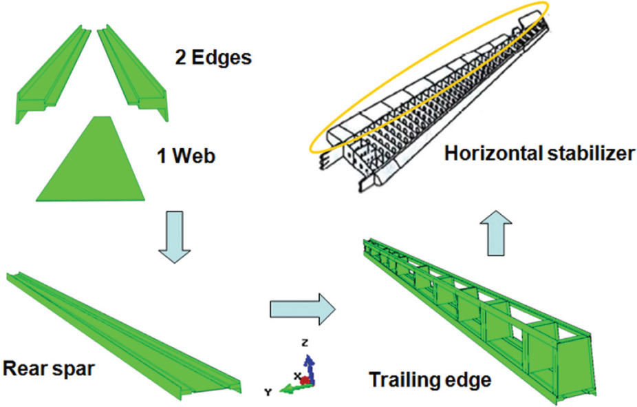
Assembly hierarchy from edge, rear spar, trailing edge to horizontal stabilizer.

The rear spar in the horizontal stabilizer and the test structure built in the laboratory have similar structural characteristics. Their common point is that the initial bulk residual stress in raw material dominates the component distortion and has an impact on subsequent assembly deformation. Ribs affect the cross-section shape of trailing edge, while axial shape is guaranteed by these much thicker edges on the rear spar. The edges are extremely long components with variable cross-section, their length-width ratio exceeding 200:1. Controlling the shape of edge is a challenge for both machining and assembling as geometric requirement.

Field measuring experiment for main edge and further simulation

The raw material of the edge on the rear spar is thick plate of AA7075. The surface residual stresses are measured at the bottom and side locations. ²⁴ The cross-sectional “T” shape is not rectangular exactly like the one of material samples used in the laboratory. It can be handled by dividing into two parts, the major upper and the minor bottom bulks. The estimated residual stress profiles are introduced to these two parts in the rolling and transverse directions, respectively. Simulated machining is followed, and the final edge has 14,100 elements approximately with 10-mm level for meshing size. The warping of the edge’s small end is 49 mm, which is within the scope of field measurement (0–10 cm). Selective surface points on the bottom section of the machined edge present compressive stress state with values around 50 MPa which are consistent with simulation results. In view of the considerable uncertainty for the edge with such substantial size, the basic analysis approach we adopt is assumed to result in acceptable prediction compared with field experimental measurement.

The component state obtained through this measurement of the specific piece of blank and subsequent scientific processing is treated as the benchmark, and thus, the initial stress profiles added in the material are regarded as the baselines of further stress fluctuations. According to the geometric shape of the as-machined edge component, the variation of residual stress in the upper bulk of raw material is expected to exert more influence on the component distortion and assembly deformation. Boundary conditions are applied to the big ends of edges, and these regions are constrained to remain fixed (have zero displacement and/or rotation) during the simulation.

Scope of the article

This article focuses on the thicker edges of the rear spar as the unique part variation responsible for consequent assembly variation of the trailing edge. Other components like the web, 11 ribs and 2 thinner edges are all built with nominal geometric dimension in FE model; thus, we exclude these part variations and only highlight the main one for frame assembly. The effect on assembly variation induced by the rib’s distortion was studied by Wang and Ding ²⁸ using full factorial design and FEA.

There are some thinner areas in the thick edges remained to be joined with thin web. Since the portion with considerable thickness accounts for the bulk of the whole assembly structure comparatively, it is reasonable to ignore the impact caused by joining operation. The rivets are modeled as binding agents in the simulation through which the gap is closed and the two points in space are joined merely. Non-linear local effect of riveting illustrated in other study is not investigated here. ²⁹

Our initial attempt underlined the importance of introducing residual stress factor into the assembly model of trailing edge. The impact of the edge’s residual stress on assembly deformation was decoupled from that of the edge’s distortion. ²⁴ We continue the study herein by taking residual stress fluctuations in the upper bulk of edge’s raw material into considerations and elicit the better match problem of main edge components’ selection aiming for better outcome of assembling frame structure.

Mathematical representation

Bulk stress fluctuation representation: Legendre polynomial combination

The Legendre polynomials are a set of orthogonal functions, and each Legendre polynomial $P_n(x)$ is an nth-degree polynomial. $P_0-P_8$ are chosen as basis functions listed in equation (1). The polynomials above $P_2$ inherently satisfy force and moment equilibrium ${\int }_{-T/2}^{T/2}{P}_i\mathrm{dx}=0$ and ${\int }_{-T/2}^{T/2}{P}_{i}x\mathrm{dx}=0$ (T is total thickness), which make them excellent options as stress components ³⁰

$$\begin{array}{cc}\multicolumn{1}{c}{}& P_0=1\hfill \\ \multicolumn{1}{c}{}& P_1=x\hfill \\ \multicolumn{1}{c}{}& P_2=\frac{1}{2}(3x^2-1)\hfill \\ \multicolumn{1}{c}{}& P_3=\frac{1}{2}(5x^3-3x)\hfill \\ \multicolumn{1}{c}{}& P_4=\frac{1}{8}(35x^4-30x^2+3)\hfill \\ \multicolumn{1}{c}{}& P_5=\frac{1}{8}(63x^5-70x^3+15x)\hfill \\ \multicolumn{1}{c}{}& P_6=\frac{1}{16}(231x^6-315x^4+105x^2-5)\hfill \\ \multicolumn{1}{c}{}& P_7=\frac{1}{16}(429x^7-693x^5+315x^3-35x)\hfill \\ \multicolumn{1}{c}{}& P_8=\frac{1}{128}(6435x^8-12012x^6+6930x^4-1260x^2+35)\hfill \end{array}$$

(1)

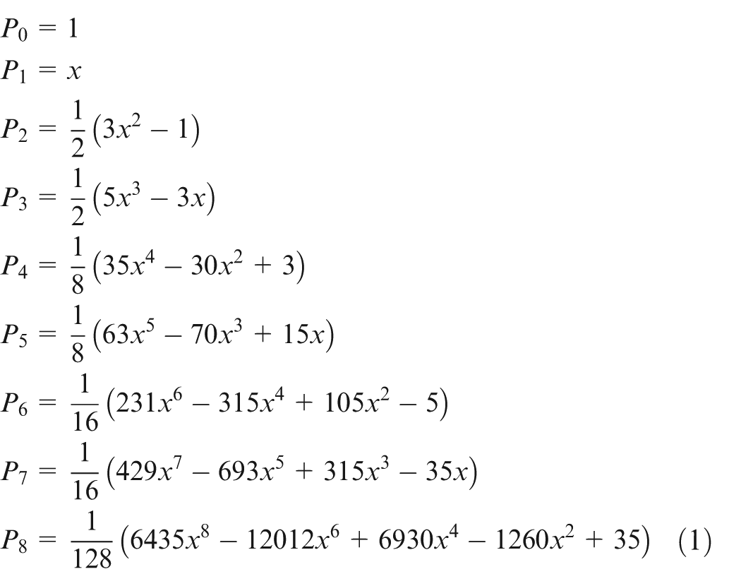
The Legendre polynomials range from [−1, 1] for both values on the X- and Y-axis representing thickness and stress, respectively; therefore, they can be considered as normalized stress distribution pattern (see Figure 4). $P_2-P_8$ represents non-linear stress distribution patterns through thickness.

Figure 4.

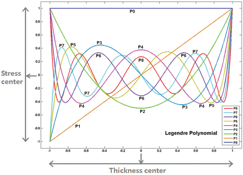
Legendre polynomials from P0 to P8.

The basic analysis approach using normalized stress profile and regression relation combined with practical surface stress measurement only provides an estimation of internal bulk residual stress in aluminum alloy plate. It might not strictly satisfy force and moment equilibrium. ABAQUS checks the solution’s equilibrium state given the selected resolution and stress redistribution will happen naturally leading to tiny adjustment. Fine-meshing plots the stress profile formulation more fully, but cost and precision must be balanced. Equation (2) describes the residual stress in equilibrium mathematically

$$\mathrm{Stress}={\displaystyle \sum _{i=2}^8}{\omega }_i·P_i$$

(2)

Here, ${\omega }_i$ is the weight coefficient of the corresponding $P_i$ which represents a decomposed stress component form. $P_0$ does not satisfy force equilibrium and only satisfies moment equilibrium, while $P_1$ does not satisfy moment equilibrium and only satisfies force equilibrium. Thus, $P_0$ and $P_1$ have not been taken into account in equation (2). This equation is also a natural result of the FE solution representing residual stress state after equilibrium analysis in ABAQUS.

It should be noted that the additional residual stress fluctuation superposed upon the baselines of stress profiles also needs to satisfy the force and moment equilibrium as inherent internal stress locked into the materials. The symmetric $P_2$ and $P_4$ share the similarity with the basic shape of baselines, while $P_6$ and $P_8$ can be viewed as higher-order symmetric stress component perturbation.

Large-scale deformation representation: Spline function fitting

The overall deformation projected in one direction forms a particular curve along a continuous measuring path on the edge. Since the edge is very long and ribs are assembled with various lengths of intervals, piecewise polynomials, like B-Spline functions, suggest themselves as suitable fitting mathematical tool for frame structure assembly.

B-Spline basis functions of various orders have different local scopes. For example, a B-Spline function of order 6 is specified by 7 equidistant knots, and it consists of 6 polynomials pieces, each of degree 5. If the measuring path is equally segmented into 10 units, one B-Spline function of order 6 occupies 6 units with knot sequence [0, 1, 2, 3, 4, 5, 6]. Through changing the knot deployment by unit translation, total 15 basis functions are needed to cover the measuring path with their respective local effects. Each piecewise deformation curve of unit length can be fitted by six non-linear polynomials to guarantee accuracy. The overall knot sequence can be combined and represented by [−5, −4 … 0, 1 … 14, 15] which is an arithmetic progression.

The whole curve thus can be represented by least-squares Spline approximation with certain precision in equation (3). Herein, n is the number of required Spline basis functions. As shown in Figure 5, for example, every B-Spline function of order 6 occupying 6 units corresponds to one control coefficient $c_j$ and total n is 15. Each $c_j$ affects the local deformation covered by the corresponding $B_j$ . The popular choice for the order is 4, and that gives a cubic Spline consisting of four polynomials pieces with equidistant knot sequence [0, 1, 2, 3, 4]. Therefore, the whole path requires 13 control coefficients over the knot sequence [−3, −2, −1, 0, 1 … 11, 12, 13]. The set of the coefficients $c_j$ combined with the chosen Spline basis functions can be obtained from optimal fitting using available deviation data. More complicated knot arrangement can be non-equidistant, and the multiplicity of the knots governs the smoothness of the curve. ³¹ Through Spline fitting, only few coefficients can imply the geometric relation of considerable discrete points extracted from the measuring path. The set of these coefficients represents deformation pattern adequately based on certain Spline basis functions

$$\mathrm{Deformation}={\displaystyle \sum _{j=1}^n}{c}_j·B_j$$

(3)

Figure 5.

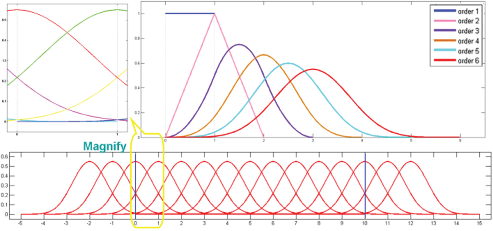
B-Spline basis of order 6 with equidistant knot deployment along normalized path.

Deformation pattern herein is also recognized at two levels, the adopted Spline basis functions and the corresponding weight coefficients. The former are characterized through knot sequence. It also can be determined from production data or simulation result preliminarily. The knot sequence choice is not unique obviously. In accordance with specific structural features, it is possible to construct the corresponding knot sequence for a specific assembly station configuration with some precision, like 0.1 mm, which means the fitting error for each point does not exceed 0.1 mm. To accomplish higher accuracy level, knot positions can be adjusted. Then the selection of knot sequence is fixed acting as the “skeleton” of deviation data. It can be chose through optimization algorithms provided by mathematical software like MATLAB Toolbox. ³¹ The weight coefficient can be viewed as random variable. If assigned a deterministic value set, the exact deviation is described via equation (3). Statistically speaking, the fluctuation of coefficient variables reflects the variation of overall deformation situation. A set of variations of coefficients should not go beyond the bounds of coefficient tolerance combination which can be transformed from original geometric tolerance of shape with consistent Spline basis functions. If single coefficient is out of tolerance, the corresponding local area is affected and points lying within it are correlated. Geometric covariance is effectively retained.

Application to main edges

Since the integral warping of trailing edge’s frame structure is caused by initial distorted edges mainly, it is important to trace the edge’s situation from fabrication process to assembly process. The same baselines of the bulk stress profiles stated above are added to the two thicker edges’ raw materials, and consequently, the component deformation are almost identical (stage 0). The displacements of two edges, that is, Edge-L and Edge-R, have opposite values shown in Figure 6 because they are represented in the global coordinate system of the assembly structure. The wedge structure of rear spar leads to different deviations of the two edges after assembly (stage 1). The stiffness of the frame structure becomes higher in terms of trailing edge which is like box girder. The deformation tendencies of the two edges turn alike with nearly equal values except for those around the small end of structure (stage 2) (see Figure 6).

Figure 6.

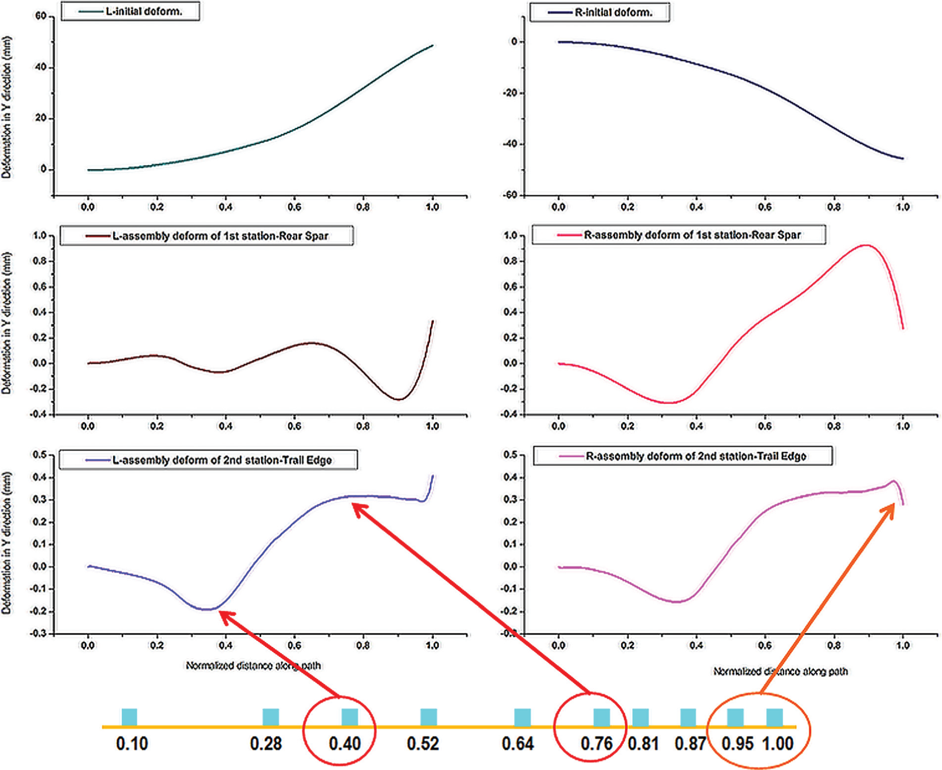
Deformation of Edge-L and Edge-R from stage 0 (component) to stages 1 and 2 (assembly).

The deformation curves of the two edges are fitted by 15 quintic B-Spline functions as described before, total number of Spline coefficients is 15 and the resultant fitting precision is 0.1 mm. All the corresponding values from stage 0 to stage 2 comprise the Spline coefficient stream which is obtained from a deterministic simulation trial (see Figure 7). This stream reveals the changes of assembly structure and reflects the evolution of the overall deformation in a compact way without loss of geometric correlation. Note that the Spline basis functions are adopted all the same here for all stages just for illustration. At stage 0, the component deformation after machining is monotonically increasing from big end to small end. At stages 1 and 2, the assembly deformation profiles go up and down several times. There is an apparent deformation pattern transition since the coefficient distributions differ greatly between them as evident from Figure 7. As for stages 1 and 2, their difference lies in moderate change of some coefficient values. The “skeleton” of deviation data can be treated identically for these two assembly stations which means the Spline basis functions can be kept the same. From a precision perspective, the initial maximum deformation of component edge is close to 50 mm, and the 0.1 mm fitting accuracy is acceptable. Meanwhile, the assembly deformation situations are within the limit of ±1 mm and some are lesser with ±0.4 mm. Thus, the maximum fitting error of 0.1 mm is not appropriate by comparison due to their close orders of magnitude. Precision requirement also urges to select different groups of Spline basis functions for component and assembly, respectively.

Figure 7.

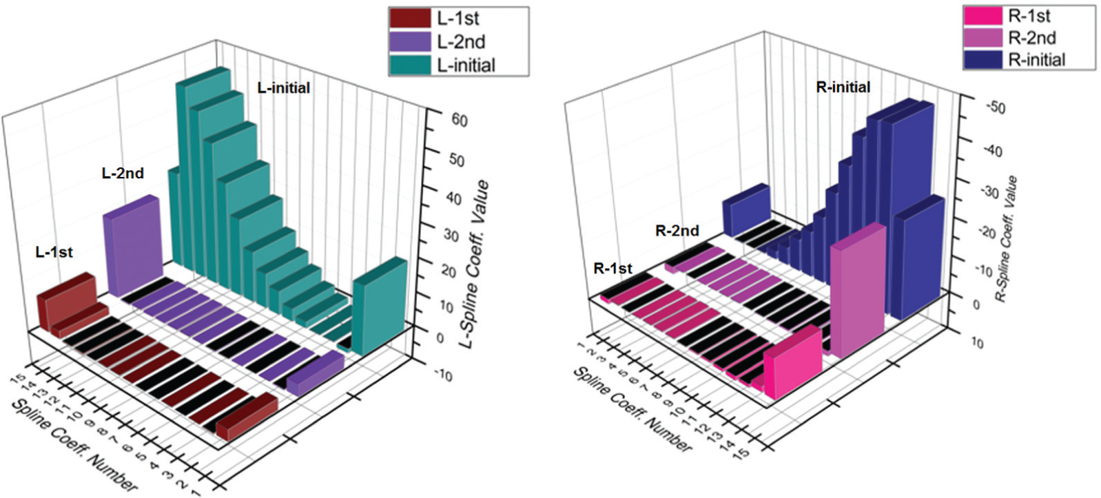
Large-scale deformation of edge represented by Spline coefficients.

The stress component perturbations can be further mapped to a practical parameter of raw material processing. Generally, the stretch ratio of Txx51 aluminum alloy plate ranges from 1.5% to 3.0%. ³² Based on the normalized residual stress profiles and regression relations as stated earlier, we can represent the resultant stress distributions of various stretch ratios utilizing weight combinations of Legendre polynomials. Some discrete stretch ratio levels in the rolling and transverse directions are calculated (see Figure 8). Herein, 3.0% is chosen as the benchmark since this situation corresponds to a smaller deviation of subsequent component status after material removal, and its specific weight coefficient combinations also correspond to the previous baselines of stress profiles that we have processed from field measurement. The differences between the weight coefficients of other levels and those of the 3.0% benchmark are plotted in Figure 8. They are approximately in a proportional pattern. The larger the stretch ratio, the bigger the stress reduction rate, and the smaller the distortion of component. The overall fluctuations of residual stress distributions can be realized through the variations of weight coefficients which correspond to the Legendre polynomials with different orders.

Figure 8.

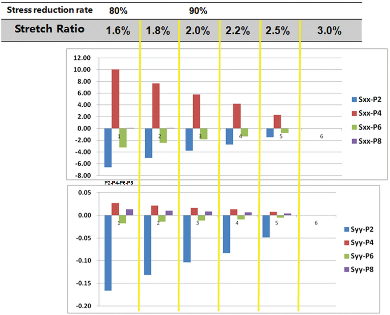
Bulk stress distribution of material represented by Legendre coefficients.

Matching optimization

Orthogonal test design via stress component fluctuation

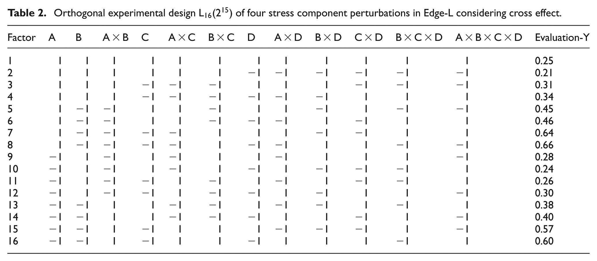
There exists uncertainty for bulk residual stress distribution in raw material. Variational initial residual stress leads to subsequent geometric variation of component and assembly. As mentioned above, the practical surface residual measurement is conducted once on one piece of edge’s material. The simulated bulk residual stress profiles taking measurement data as input after processing are reliable because the machining result can be verified in the field. We design an orthogonal test via overall stress profile fluctuation to simulate variation of bulk residual stress distribution and treat the deterministic baselines of stress profiles stated previously as trial center.

Residual stress exist within a body in the absence of any external load, the stress state must satisfy static equilibrium. Perturbed stress component is in the form of Legendre polynomial. According to the preliminary sensitivity analysis, four forms of stress fluctuations are concentrated here (Table 1).

Table 1.

Dominant stress component perturbations as four factors and the corresponding Legendre coefficient variations at two levels.

Letter code	Factor (4)	Level (2)	Legendre coefficient variation	Remark
A	Syy-All	1	1.1	10% perturbation (multiple for all)
		−1	0.9
B	Sxx-P2	1	−3.42	10% perturbation (addition or subtraction of single stress component)
		−1	3.42
C	Sxx-P4	1	5.21
		−1	−5.21
D	Sxx-P6	1	−1.67
		−1	1.67

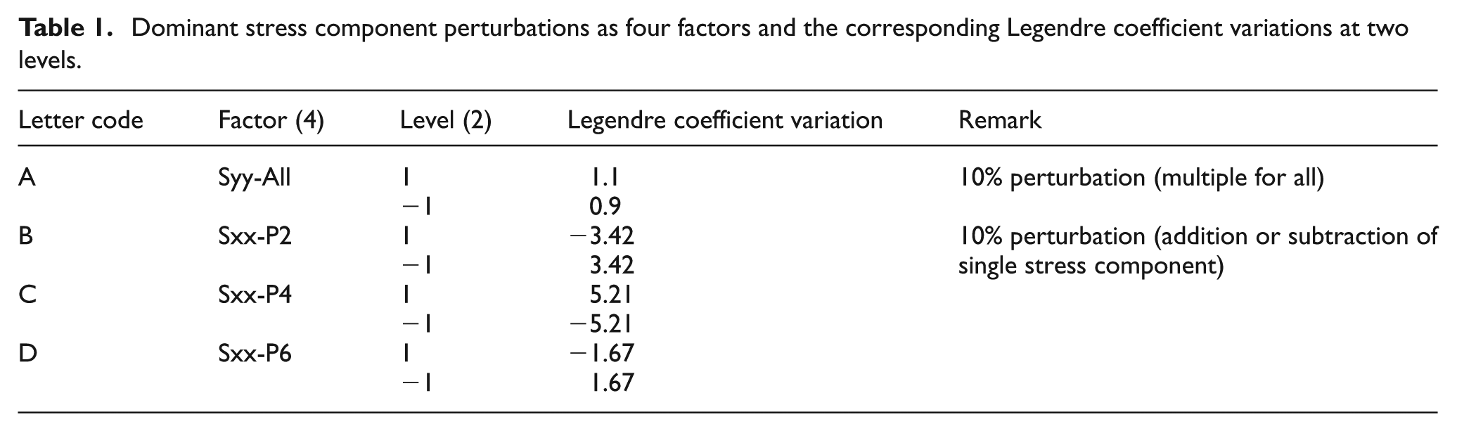
Syy-All means the integral stress distribution in the transverse direction. Sxx-P2, Sxx-P4 and Sxx-P6 means respective stress distribution pattern in the rolling direction represented by the corresponding Legendre polynomial function. We assume these four factors are independent in the orthogonal test design. ±10% fluctuation of stress value is regarded as variation range of the factors. For Syy-All, integral stress without decomposition is multiplied by 1.1 and 0.9, respectively, representing two levels. For Sxx-P2, Sxx-P4 and Sxx-P6, the trial center’s corresponding Legendre coefficient is adjusted by adding and subtracting 10% of its value, respectively, simulating single stress component perturbation. For example, the coefficient of $P_2$ in the rolling direction is −34.19, and then the amplitude of perturbation is 3.419 leading to −37.609 or −30.771 as perturbed weight for $P_2$ . In order that every level of each factor is coded “equally” and not affected by difference among multiple, addition, and subtraction of weight coefficient variations, the corresponding canonical variables whose value range is [−1, 1] for all are used for substituting natural variables in order to simplify next regression analysis.

The orthogonal table using ${\mathrm{L}}_{16}(2^{15})$ is designed where A, B, C, and D are letter codes for four factors (Table 2). Total 16 simulation experiments are required. The above stress fluctuations only apply to Edge-L, and Edge-R remains the trial center level, that is, the baseline. Different matches of these two thicker edges lead to different assembly deformation situations.

Table 2.

Orthogonal experimental design ${\mathrm{L}}_{16}(2^{15})$ of four stress component perturbations in Edge-L considering cross effect.

Factor	A	B	A × B	C	A × C	B × C	D	A × D	B × D	C × D	B × C × D	A × B × C × D	Evaluation-Y
1	1	1	1	1	1	1	1	1	1	1	1	1	0.25
2	1	1	1	1	1	1	−1	−1	−1	−1	−1	−1	0.21
3	1	1	1	−1	−1	−1	1	1	1	−1	−1	−1	0.31
4	1	1	1	−1	−1	−1	−1	−1	−1	1	1	1	0.34
5	1	−1	−1	1	1	−1	1	1	−1	1	−1	−1	0.45
6	1	−1	−1	1	1	−1	−1	−1	1	−1	1	1	0.46
7	1	−1	−1	−1	−1	1	1	1	−1	−1	1	1	0.64
8	1	−1	−1	−1	−1	1	−1	−1	1	1	−1	−1	0.66
9	−1	1	−1	1	−1	1	1	−1	1	1	1	−1	0.28
10	−1	1	−1	1	−1	1	−1	1	−1	−1	−1	1	0.24
11	−1	1	−1	−1	1	−1	1	−1	1	−1	−1	1	0.26
12	−1	1	−1	−1	1	−1	−1	1	−1	1	1	−1	0.30
13	−1	−1	1	1	−1	−1	1	−1	−1	1	−1	1	0.38
14	−1	−1	1	1	−1	−1	−1	1	1	−1	1	−1	0.40
15	−1	−1	1	−1	1	1	1	−1	−1	−1	1	−1	0.57
16	−1	−1	1	−1	1	1	−1	1	1	1	−1	1	0.60

Comprehensive evaluation of multi-objective problem

For better match, some evaluation targets need to be identified first for this assembly case. The measuring paths along two thinner edges, Edge-M and Edge-N, are constructed, respectively, which are composed of considerable discrete nodes on the surface. Two aspects of deviation in the Y direction concerning them are focused (see Figure 9). Let $d_M$ and $d_N$ be the deviation value vector of two measuring path with same array size. One aspect is the deviation of the axis position of these two edges listed as equation (4). Another is the deviation of the gap distance between these two edges listed as equation (5)

$$d_{\mathrm{axis}}=0.5\times (d_M+d_N)$$

(4)

$$d_{\mathrm{gap}}=d_M-d_N$$

(5)

Figure 9.

Geometric evaluation for overall deformation after assembly.

In order to examine the deviation magnitude regardless of its direction, that is, positive or negative, we calculate the average of all the vector components’ absolute values, respectively. Then we obtain two geometric evaluation targets; the smaller the targets, the better the assembly matches. This is a multi-objective optimization problem for better match. A comprehensive evaluation needs to be created equally referring to these two targets. The difference in the order of magnitude between them is first adjusted and the root mean square of the two adjusted values is calculated as final evaluation object. Total 16 evaluation results of simulation experiments can be obtained after data processing, and they are displayed at the rightmost column in Table 2.

Orthogonal regression analysis for better match

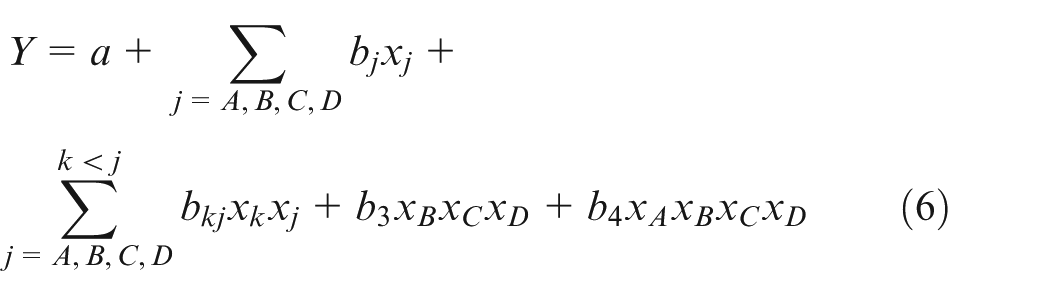
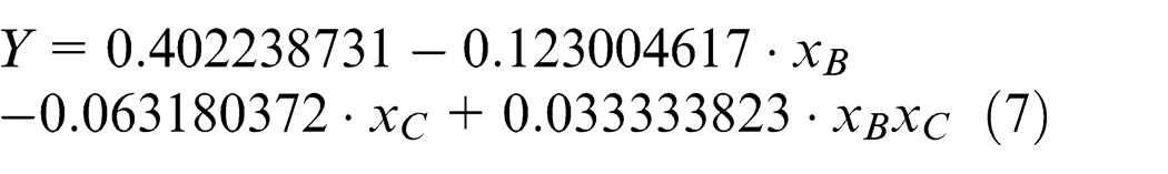
The regression equation takes the following form as shown in equation (6). The coefficients can be obtained through least-square regression and the corresponding analysis of variance (ANOVA) is shown in Table 3. It is apparent that most terms do not indicate statistical significance. We select those with highest significance and simplify the regression equation listed as in equation (7)

$$Y=a+\sum _{j=A,B,C,D}{b}_j{x}_j+{\displaystyle \sum _{j=A,B,C,D}^{k<j}}{b}_{\mathrm{kj}}{x}_k{x}_j+b_3{x}_B{x}_C{x}_D+b_4{x}_A{x}_B{x}_C{x}_D$$

(6)

$$Y=0.402238731-0.123004617·x_B-0.063180372·x_C+0.033333823·x_B{x}_C$$

(7)

Table 3.

ANOVA for the first round with all factors and their cross terms.

Factor	SS	df	MS	F	Significance
A	0.005731013	1	0.005731013	11.96134568	*
B	0.242082172	1	0.242082172	505.2559364	**
(A × B)	0.002634111	1	0.002634111	5.49772181
C	0.063868151	1	0.063868151	133.3008624	**
(A × C)	0.001388623	1	0.001388623	2.898230968
(B × C)	0.0177783	1	0.0177783	37.10554737	**
D	0.000391743	1	0.000391743	0.817616718
(A × D)	5.95199E-06	1	5.95199E-06	0.012422544
(B × D)	0.000603651	1	0.000603651	1.259896255
(C × D)	0.00146924	1	0.00146924	3.066488389
(B × C × D)	0.001048782	1	0.001048782	2.188940168
(A × B × C × D)	1.633E-11	1	1.633E-11	3.40827E-08
Regression	0.337001739	12	0.028083478	58.61375073	**
Error	0.001437383	3	0.000479128
Summation	0.338439122	16−1 = 15
F0.05(1, 3) = 10.13, F0.01(1, 3) = 34.12, F0.05(12, 3) = 8.74, F0.01(12, 3) = 27.05

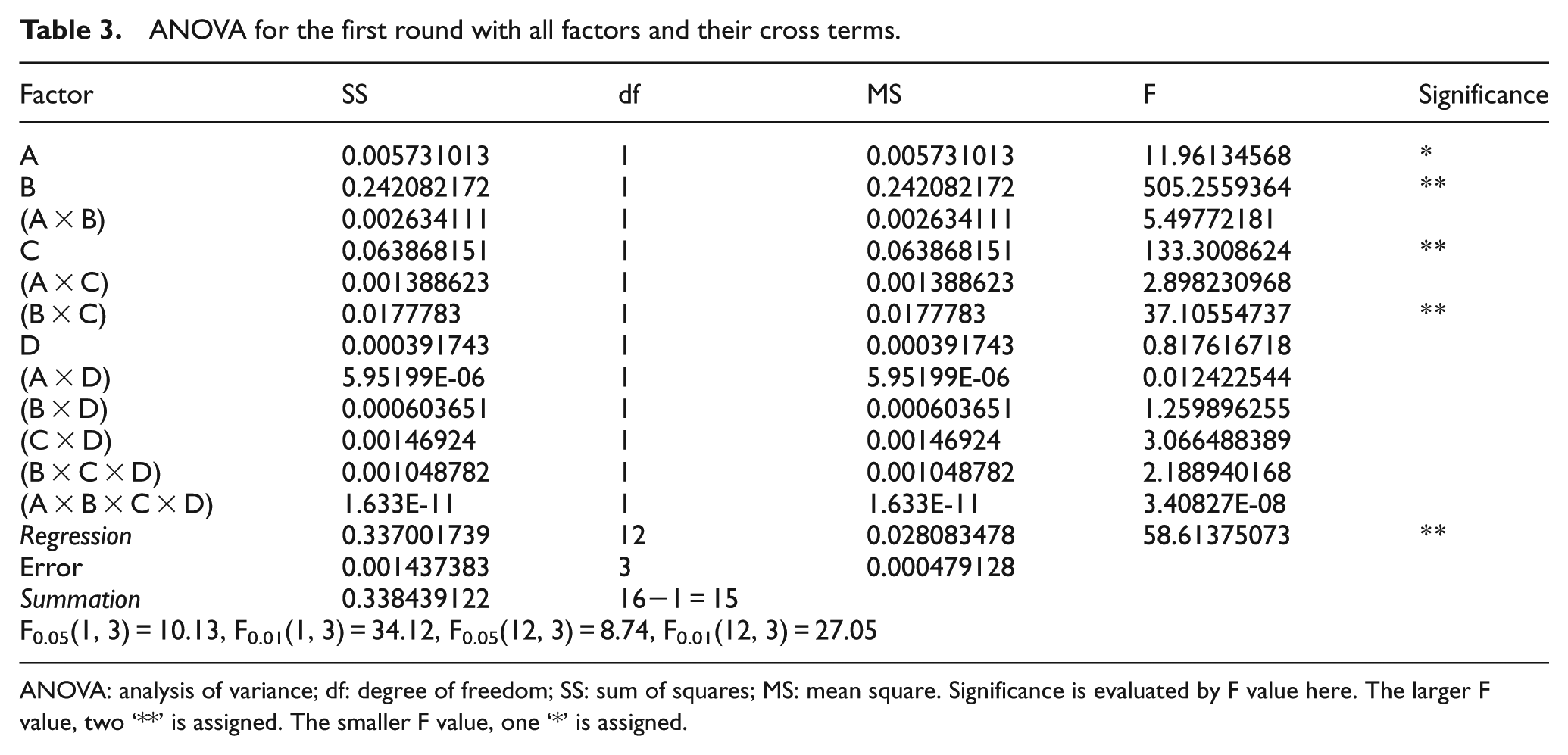
ANOVA: analysis of variance; df: degree of freedom; SS: sum of squares; MS: mean square. Significance is evaluated by F value here. The larger F value, two ‘**’ is assigned. The smaller F value, one ‘*’ is assigned.

We then perform second round of ANOVA as can be seen in Table 4. The regression relation between Sxx-P2, Sxx-P4, their product term and comprehensive evaluation target is of great significance statistically. The order of influence is B > C > B × C. It should be noted that the product term does not have physical meaning because both Sxx-P2 and Sxx-P4 take effect leading to the superposition of stress fluctuation in the rolling direction.

Table 4.

ANOVA for the second round with main factors.

Factor	SS	df	MS	F	Significance
B	0.242082172	1	0.242082172	197.4770502	**
C	0.063868151	1	0.063868151	52.10005307	**
B × C	0.0177783	1	0.0177783	14.50253923	**
Regression	0.323728623	3	0.107909541	88.02654749	**
Error	0.0147105	12	0.001225875
Summation	0.338439122	16−1 = 15
F0.05(1, 12) = 4.75, F0.01(1, 12) = 9.33, F0.05(3, 12) = 3.49, F0.01(3, 12) = 5.95

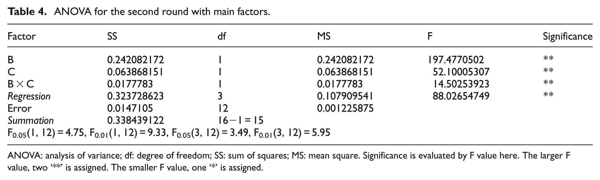
ANOVA: analysis of variance; df: degree of freedom; SS: sum of squares; MS: mean square. Significance is evaluated by F value here. The larger F value, two ‘**’ is assigned. The smaller F value, one ‘*’ is assigned.

To minimize Y for better match, $x_B$ and $x_C$ as canonical variables are taken value of 1 for both. It means that when Edge-R is at trial center level, Edge-L is better to have 10% Sxx-P2 and Sxx-P4 stress component perturbation in its raw material for the sake of controlling assembly deformation. We optimize the variations of the corresponding Legendre coefficient for better match, namely, −3.42 of Sxx-P2 and 5.21 of Sxx-P4 representing 10% perturbation.

Mapping relation

Assembly deformation prediction for better match

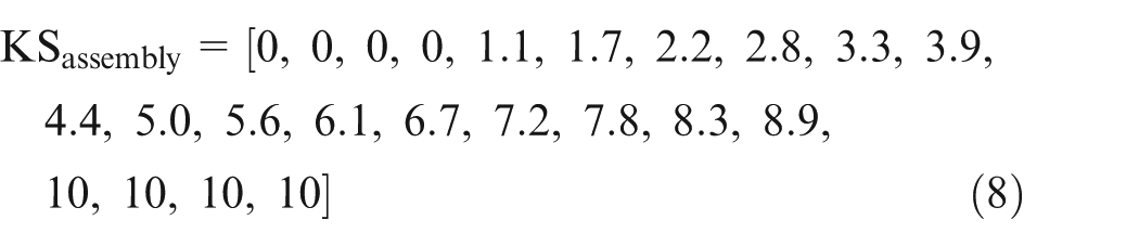
The overall deformation of stage 2 is evaluated using the axis position between Edge-M and Edge-N as described previously. A total of 16 simulated deformation results are represented via certain Spline basis functions and corresponding Spline coefficients. The same proper knot sequence is obtained for two assembly stages through MATLAB Spline Toolbox automatically when realizing cubic Spline fitting listed in equation (8). The required number of coefficients is 19, and the precision reaches 0.005 mm which means maximum fitting error for every point on the measuring path does not exceed that quantity. Manual insertion of knots around the rib positions on the measuring path of assembly can also be made to adjust the required local approximation accuracy if necessary

$${\mathrm{KS}}_{\mathrm{assembly}}=[0,0,0,0,1.1,1.7,2.2,2.8,3.3,3.9,4.4,5.0,5.6,6.1,6.7,7.2,7.8,8.3,8.9,10,10,10,10]$$

(8)

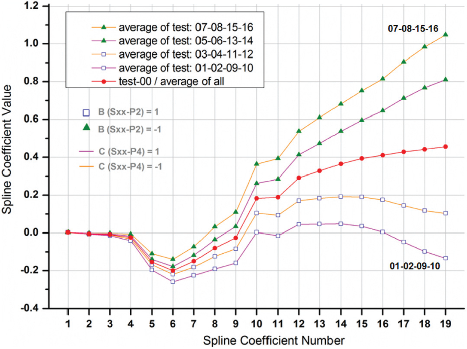
The Spline coefficient distributions are visible in Figure 10. Assembly deformation patterns are clearly depicted in this way. The discrepancies mainly lie in the constricted section of the trailing edge reflected by a divergent tail shape in the Spline coefficient distributions. According to the optimization result for better match, factors B and C should be equal to 1, and the situations should correspond to simulation experiments test-01, test-02, test-09 and test-10. We observe that these four tests profiles are located below the trial center line and occupy the bottom area of the divergent tail.

Figure 10.

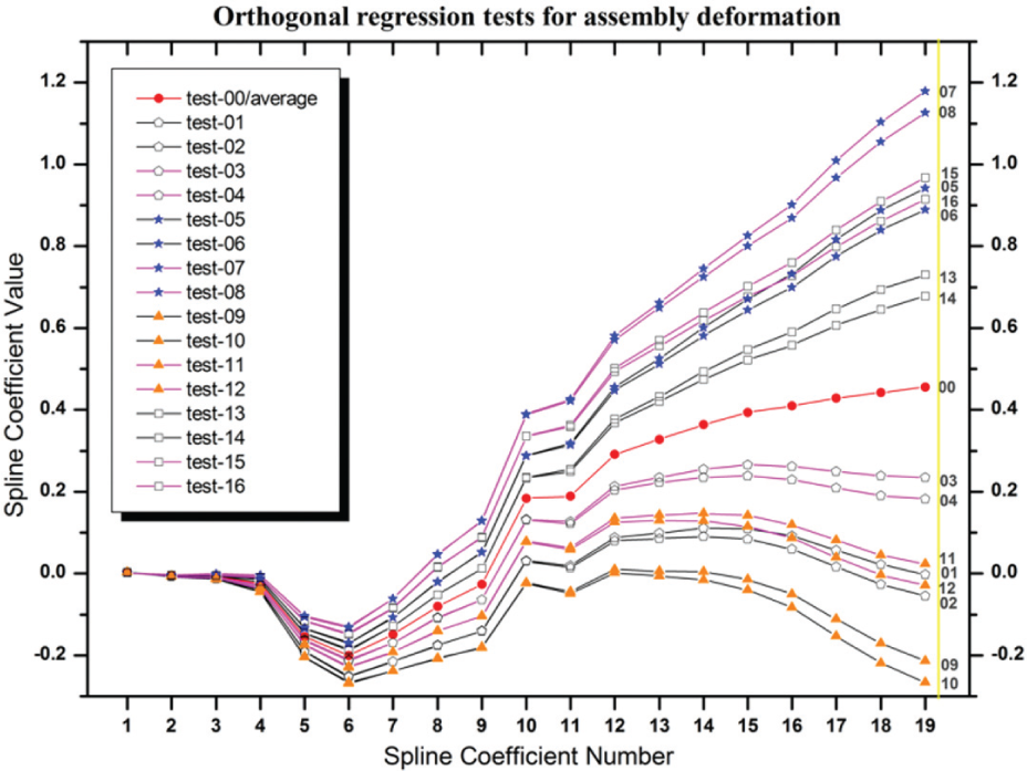
Orthogonal regression tests for assembly deformation of Edge-M and Edge-N axes.

This area representing better assembly results is magnified separately, displayed in Figure 11. Here four test profiles are also the outputs of the orthogonal experiment design concerning factors A and D. The example profile shown in red is the average of test-01, test-02, test-09 and test-10. Inspection of Figure 11 indicates that factor A has influence on most Spline coefficients since the pentagon marker and triangle marker do not overlap from the fourth coefficient approximately; factor D has influence on last nine Spline coefficients since the black tag line and the turquoise tag line split from the 10th coefficient approximately. The assembly deformation pattern change induced by the stress component perturbation can be analyzed graphically revealing the region of influence. The quantitative relation can be formulated through mapping scheme between Legendre coefficients and Spline coefficients described ins equation (9)

$$\mathrm{For}\mathrm{assembly}:{\left[\begin{array}{c}\hfill {\mathrm{sc}}_{01}\hfill \\ \multicolumn{1}{c}{{\mathrm{sc}}_{02}}\\ \multicolumn{1}{c}{⋮}\\ \multicolumn{1}{c}{{\mathrm{sc}}_{10}}\\ \multicolumn{1}{c}{{\mathrm{sc}}_{11}}\\ \multicolumn{1}{c}{⋮}\\ \multicolumn{1}{c}{{\mathrm{sc}}_{19}}\end{array}\right]}_{19\times 1}=\left[\begin{array}{c}\hfill {\overline{\mathrm{sc}}}_{01}\hfill \\ \multicolumn{1}{c}{{\overline{\mathrm{sc}}}_{02}}\\ \multicolumn{1}{c}{⋮}\\ \multicolumn{1}{c}{{\overline{\mathrm{sc}}}_{10}}\\ \multicolumn{1}{c}{{\overline{\mathrm{sc}}}_{11}}\\ \multicolumn{1}{c}{⋮}\\ \multicolumn{1}{c}{{\overline{\mathrm{sc}}}_{19}}\end{array}\right]+\frac{1}{2}·x_A·\left[\begin{array}{c}\hfill 0\hfill \\ \multicolumn{1}{c}{0}\\ \multicolumn{1}{c}{0}\\ \multicolumn{1}{c}{{\mathrm{r}}_{04}^{\mathrm{A}}}\\ \multicolumn{1}{c}{⋮}\\ \multicolumn{1}{c}{⋮}\\ \multicolumn{1}{c}{{\mathrm{r}}_{19}^{\mathrm{A}}}\end{array}\right]+\frac{1}{2}·x_D·\left[\begin{array}{c}\hfill 0\hfill \\ \multicolumn{1}{c}{0}\\ \multicolumn{1}{c}{⋮}\\ \multicolumn{1}{c}{⋮}\\ \multicolumn{1}{c}{{\mathrm{r}}_{11}^{\mathrm{D}}}\\ \multicolumn{1}{c}{⋮}\\ \multicolumn{1}{c}{{\mathrm{r}}_{19}^{\mathrm{D}}}\end{array}\right]$$

(9)

Figure 11.

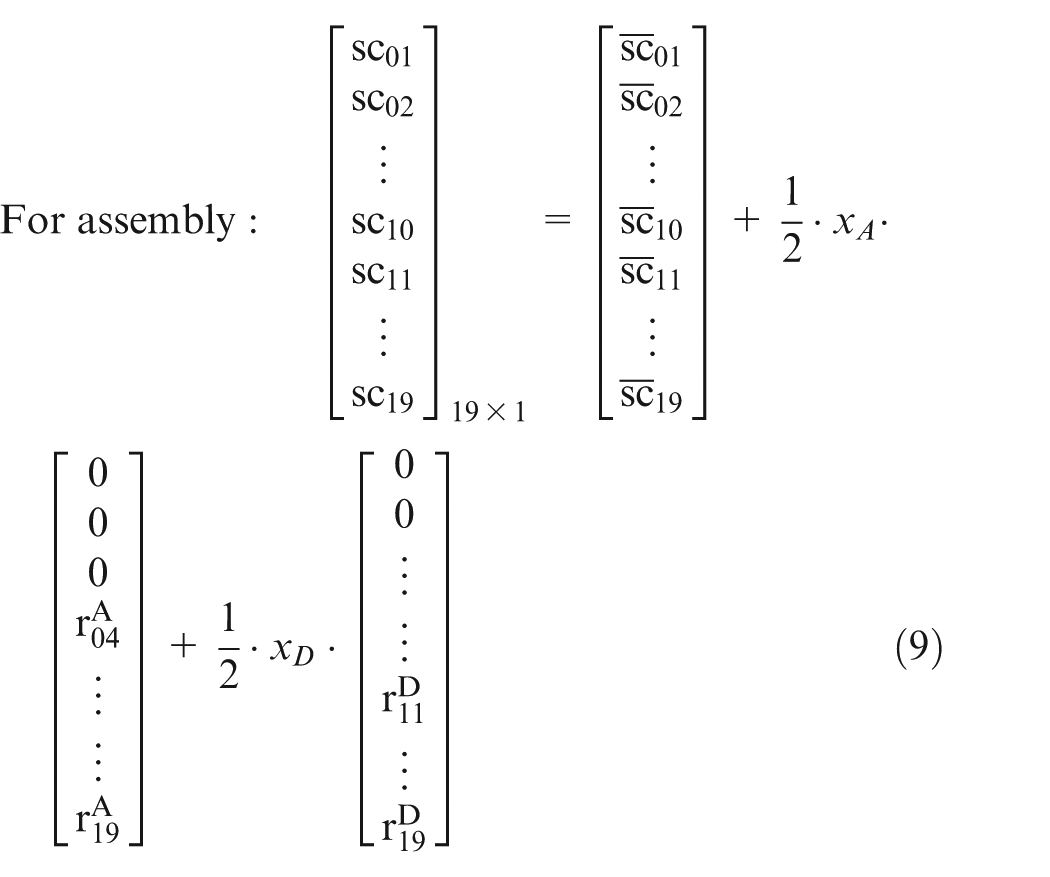
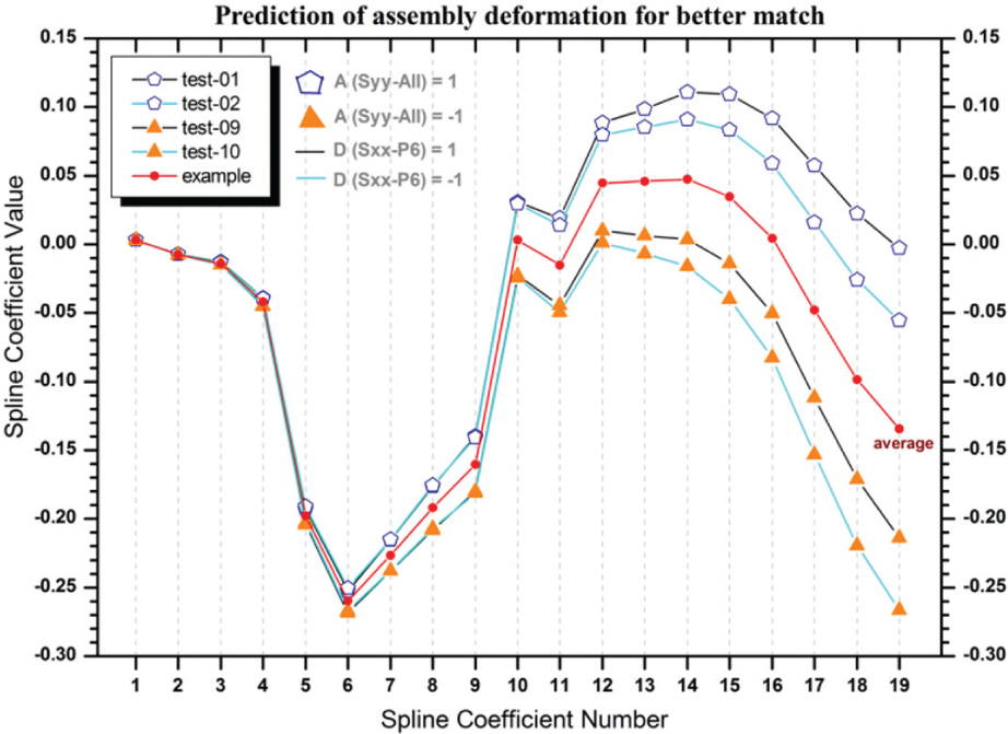
Prediction of assembly deformation for better match-minor Spline coefficients.

Here, the column on the left side of equation is the assembly Spline coefficient array to be predicted if better match occurs. $\overline{\mathrm{sc}}$ array is the average level marked as the example. $x_A$ and $x_D$ as canonical variables range from [−1, 1]. The exact variation of Legendre coefficient can be converted easily. ${\mathrm{r}}^{\mathrm{A}}$ and ${\mathrm{r}}^{\mathrm{D}}$ are the range arrays for factors A and D, respectively. Each item of the array is the variable range for corresponding Spline coefficient on the basis of each item of $\overline{\mathrm{sc}}$ as center value. For instance, ${\mathrm{r}}_{04}^{\mathrm{A}}$ is the interval or difference of the fourth Spline coefficient’s average value between test-01, test-02 and test-09, test-10, while ${\mathrm{r}}_{11}^{\mathrm{D}}$ is that of the 11th Spline coefficient’s average value between test-01, test-09 and test-02, test-10. Zero means no influential effect on the local region which is controlled by the corresponding Spline coefficient.

The orthogonal experiment combinations concerning only factors B and C from all 16 tests are further processed. The corresponding Spline coefficient distributions dealing with each average level of every four tests are shown in Figure 12

Figure 12.

Prediction of assembly deformation for better match-major Spline coefficients.

As for the $\overline{\mathrm{sc}}$ array, it can be viewed as a function of major influential factors, factors B and C. The specific $\overline{\mathrm{sc}}$ in equation (9) is the array substituting $x_B=x_C=1$ in equation (10). The first column on the right side of equation is the trial center as test-00. ${\mathrm{r}}^{\mathrm{B}}$ and ${\mathrm{r}}^{\mathrm{C}}$ are the range arrays for factors B and C, respectively. For example, each item of ${\mathrm{r}}^{\mathrm{B}}$ is the interval or difference of the corresponding Spline coefficients’ average values between test-01, test-02, test-09, test-10, test-03, test-04, test-11, test-12 and test-05, test-06, test-13, test-14, test-07, test-08, test-15, test-16

$$\left[\begin{array}{c}\hfill {\overline{\mathrm{sc}}}_{01}\hfill \\ \multicolumn{1}{c}{{\overline{\mathrm{sc}}}_{02}}\\ \multicolumn{1}{c}{⋮}\\ \multicolumn{1}{c}{{\overline{\mathrm{sc}}}_{10}}\\ \multicolumn{1}{c}{{\overline{\mathrm{sc}}}_{11}}\\ \multicolumn{1}{c}{⋮}\\ \multicolumn{1}{c}{{\overline{\mathrm{sc}}}_{19}}\end{array}\right]=\underset{\mathrm{test}-00}{\left[\begin{array}{c}\hfill {\mathrm{sc}}_{01}\hfill \\ \multicolumn{1}{c}{{\mathrm{sc}}_{02}}\\ \multicolumn{1}{c}{⋮}\\ \multicolumn{1}{c}{{\mathrm{sc}}_{10}}\\ \multicolumn{1}{c}{{\mathrm{sc}}_{11}}\\ \multicolumn{1}{c}{⋮}\\ \multicolumn{1}{c}{{\mathrm{sc}}_{19}}\end{array}\right]}+\frac{1}{2}·x_B·\left[\begin{array}{c}\hfill 0\hfill \\ \multicolumn{1}{c}{{\mathrm{r}}_{02}^{\mathrm{B}}}\\ \multicolumn{1}{c}{⋮}\\ \multicolumn{1}{c}{⋮}\\ \multicolumn{1}{c}{⋮}\\ \multicolumn{1}{c}{⋮}\\ \multicolumn{1}{c}{{\mathrm{r}}_{19}^{\mathrm{B}}}\end{array}\right]+\frac{1}{2}·x_C·\left[\begin{array}{c}\hfill 0\hfill \\ \multicolumn{1}{c}{0}\\ \multicolumn{1}{c}{{\mathrm{r}}_{03}^{\mathrm{C}}}\\ \multicolumn{1}{c}{⋮}\\ \multicolumn{1}{c}{⋮}\\ \multicolumn{1}{c}{⋮}\\ \multicolumn{1}{c}{{\mathrm{r}}_{19}^{\mathrm{C}}}\end{array}\right]$$

(10)

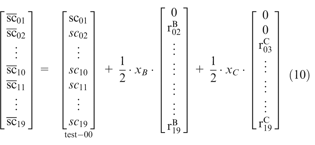
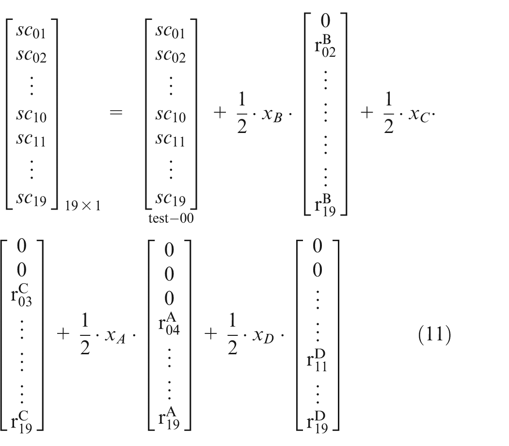
We can get the comprehensive formula equation (11) combined with equations (9) and (10)

$${\left[\begin{array}{c}\hfill {\mathrm{sc}}_{01}\hfill \\ \multicolumn{1}{c}{{\mathrm{sc}}_{02}}\\ \multicolumn{1}{c}{⋮}\\ \multicolumn{1}{c}{{\mathrm{sc}}_{10}}\\ \multicolumn{1}{c}{{\mathrm{sc}}_{11}}\\ \multicolumn{1}{c}{⋮}\\ \multicolumn{1}{c}{{\mathrm{sc}}_{19}}\end{array}\right]}_{19\times 1}=\underset{\mathrm{test}-00}{\left[\begin{array}{c}\hfill {\mathrm{sc}}_{01}\hfill \\ \multicolumn{1}{c}{{\mathrm{sc}}_{02}}\\ \multicolumn{1}{c}{⋮}\\ \multicolumn{1}{c}{{\mathrm{sc}}_{10}}\\ \multicolumn{1}{c}{{\mathrm{sc}}_{11}}\\ \multicolumn{1}{c}{⋮}\\ \multicolumn{1}{c}{{\mathrm{sc}}_{19}}\end{array}\right]}+\frac{1}{2}·x_B·\left[\begin{array}{c}\hfill 0\hfill \\ \multicolumn{1}{c}{{\mathrm{r}}_{02}^{\mathrm{B}}}\\ \multicolumn{1}{c}{⋮}\\ \multicolumn{1}{c}{⋮}\\ \multicolumn{1}{c}{⋮}\\ \multicolumn{1}{c}{⋮}\\ \multicolumn{1}{c}{{\mathrm{r}}_{19}^{\mathrm{B}}}\end{array}\right]+\frac{1}{2}·x_C·\left[\begin{array}{c}\hfill 0\hfill \\ \multicolumn{1}{c}{0}\\ \multicolumn{1}{c}{{\mathrm{r}}_{03}^{\mathrm{C}}}\\ \multicolumn{1}{c}{⋮}\\ \multicolumn{1}{c}{⋮}\\ \multicolumn{1}{c}{⋮}\\ \multicolumn{1}{c}{{\mathrm{r}}_{19}^{\mathrm{C}}}\end{array}\right]+\frac{1}{2}·x_A·\left[\begin{array}{c}\hfill 0\hfill \\ \multicolumn{1}{c}{0}\\ \multicolumn{1}{c}{0}\\ \multicolumn{1}{c}{{\mathrm{r}}_{04}^{\mathrm{A}}}\\ \multicolumn{1}{c}{⋮}\\ \multicolumn{1}{c}{⋮}\\ \multicolumn{1}{c}{{\mathrm{r}}_{19}^{\mathrm{A}}}\end{array}\right]+\frac{1}{2}·x_D·\left[\begin{array}{c}\hfill 0\hfill \\ \multicolumn{1}{c}{0}\\ \multicolumn{1}{c}{⋮}\\ \multicolumn{1}{c}{⋮}\\ \multicolumn{1}{c}{{\mathrm{r}}_{11}^{\mathrm{D}}}\\ \multicolumn{1}{c}{⋮}\\ \multicolumn{1}{c}{{\mathrm{r}}_{19}^{\mathrm{D}}}\end{array}\right]$$

(11)

The mapping scheme expressed in this way contains abundant information involving non-linear stress component perturbation pattern in Legendre polynomial form and non-linear localized deformation pattern in Spline function form. It reveals not only the region of influence but also its impact magnitude via ${\mathrm{r}}^{\mathrm{B}}$ , ${\mathrm{r}}^{\mathrm{C}}$ , ${\mathrm{r}}^{\mathrm{A}}$ and ${\mathrm{r}}^{\mathrm{D}}$ range arrays. The factors B and C, that is, Sxx-P2 and Sxx-P4, are the major influential stress component forms of perturbation since less zeros are in the corresponding range arrays. And the factors A and D, that is, Syy-all and Sxx-P6, are the minor ones. The pattern mapping is achieved through a concise linear form which captures the essential of the problem sufficiently.

The exact assembly deformation prediction can be transformed from the Spline coefficient distribution pattern based on the corresponding group of Spline basis functions. The transforming results are given in Figure 13 showing the situations of 10% stress component perturbation of Sxx-P2 and Sxx-P4 for better match. The length of the measuring path for axis position is normalized where 0 means the bigger end and 1 means the smaller end of the trailing edge. The example one is the average level which can also be converted from $\overline{\mathrm{sc}}$ . The deformation profiles of test-01 and test-10 confine the scope of predicted overall assembly variation within which the better match is achieved. Naturally, the shape of their Spline coefficient distribution patterns and the overall deformation profiles are similar since the changing trend is consistently represented by Spline basis function fitting.

Figure 13.

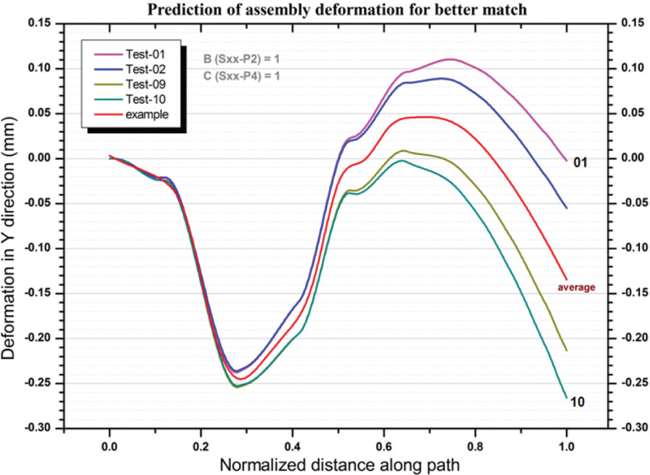
Prediction of assembly deformation for better match-corresponding warping.

Component deformation selection for better match

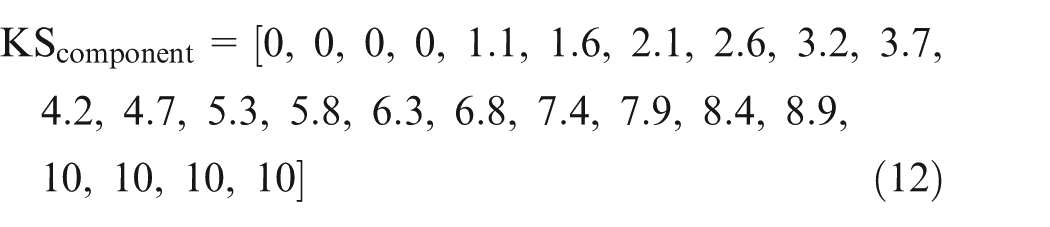
The overall component deformation situations involving test-01, test-02, test-09 and test-10 are fitted using cubic Spline functions. The proper knot sequence is also optimized via MATLAB Spline Toolbox automatically listed in equation (12). The required number of coefficients is 20, and the precision reaches 0.01 mm. Both equations (8) and (12) are set mainly from the precision aspect here

$${\mathrm{KS}}_{\mathrm{component}}=[0,0,0,0,1.1,1.6,2.1,2.6,3.2,3.7,4.2,4.7,5.3,5.8,6.3,6.8,7.4,7.9,8.4,8.9,10,10,10,10]$$

(12)

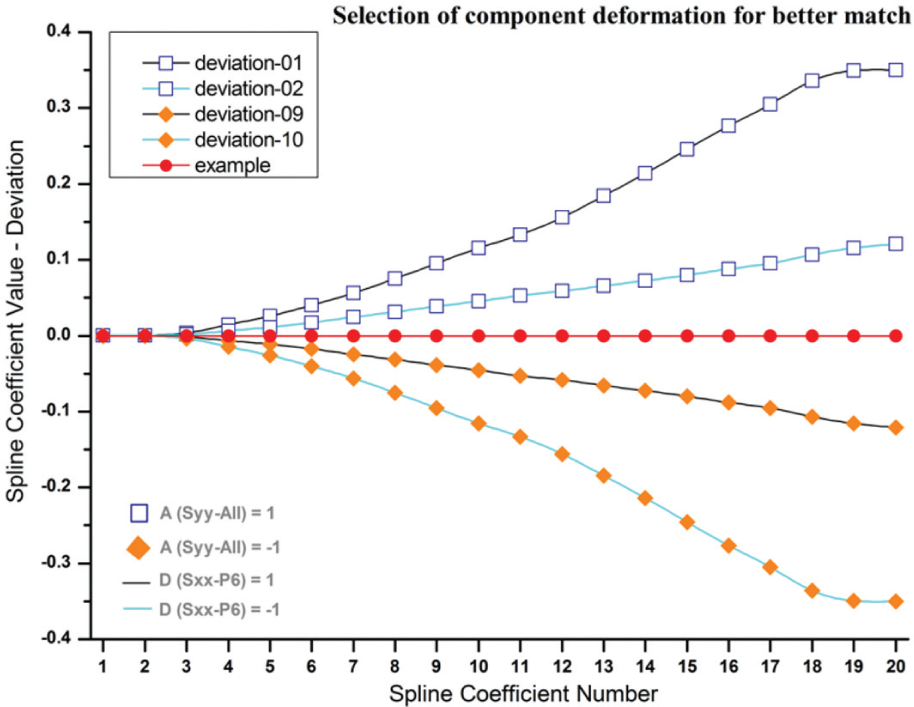
The deviation patterns of all four tests’ Spline coefficient values away from their average are shown in Figure 14. On the basis of taking value 1 for both factors B and C, the example represents this average level marked using red circles. Both factors A and D have effect on most coefficient deviations beginning from the third one approximately unlike the assembly condition where they are responsible for different sets of coefficient. The quantitative mapping relation between variational Legendre coefficients representing stress perturbation pattern and Spline coefficients representing component deformation pattern can be formulated as equation (13). The processing is handled in the same manner as that for assembly

$$\mathrm{For}\mathrm{component}:{\left[\begin{array}{c}\hfill {\mathrm{sc}}_{01}\hfill \\ \multicolumn{1}{c}{⋮}\\ \multicolumn{1}{c}{⋮}\\ \multicolumn{1}{c}{⋮}\\ \multicolumn{1}{c}{{\mathrm{sc}}_{20}}\end{array}\right]}_{20\times 1}=\left[\begin{array}{c}\hfill {\overline{\mathrm{sc}}}_{01}\hfill \\ \multicolumn{1}{c}{⋮}\\ \multicolumn{1}{c}{⋮}\\ \multicolumn{1}{c}{⋮}\\ \multicolumn{1}{c}{{\overline{\mathrm{sc}}}_{20}}\end{array}\right]+\frac{1}{2}·x_A·\left[\begin{array}{c}\hfill 0\hfill \\ \multicolumn{1}{c}{0}\\ \multicolumn{1}{c}{{\mathrm{r}}_{03}^{\mathrm{A}}}\\ \multicolumn{1}{c}{⋮}\\ \multicolumn{1}{c}{{\mathrm{r}}_{20}^{\mathrm{A}}}\end{array}\right]+\frac{1}{2}·x_D·\left[\begin{array}{c}\hfill 0\hfill \\ \multicolumn{1}{c}{0}\\ \multicolumn{1}{c}{{\mathrm{r}}_{03}^{\mathrm{D}}}\\ \multicolumn{1}{c}{⋮}\\ \multicolumn{1}{c}{{\mathrm{r}}_{20}^{\mathrm{D}}}\end{array}\right]$$

(13)

Figure 14.

Selection of component deformation for better match-Spline coefficients.

We observe from Figure 14 that if the opposite tendency happens for two factors’ levels, like the situation of $x_A=1$ and $x_D=-1$ , the deviation pattern of Spline coefficient from the average is linear with small gap, while for the same tendency situation like $x_A=1$ and $x_D=1$ , the deviation pattern presents a quadratic profile with large gap. This implies the complicated different superposition effects of stress component perturbation. It depends on the mathematical expression we define for every stress component perturbation, the specific structural feature of the edge and the component location within its raw material.

The specific component overall deformation can be transformed based on the group of Spline basis functions chosen for this stage as plotted in Figure 15. Edge-R stays at the trial center level, while the example of Edge-L is the average level to be selected for better match. The deviation profiles of test-01 and test-10 constitute the upper bound and lower bound of the overall variation range for centered average within which the better match is guaranteed. Of course, these two tests confine the optimized boundary either for assembly deformation prediction or for component deformation selection consistently considering 10% stress component perturbation of Sxx-P2 and Sxx-P4. Data in Figure 15 suggest that the Edge-L with bigger amount of small end’s warping compared with Edge-R should be selected for better match.

Figure 15.

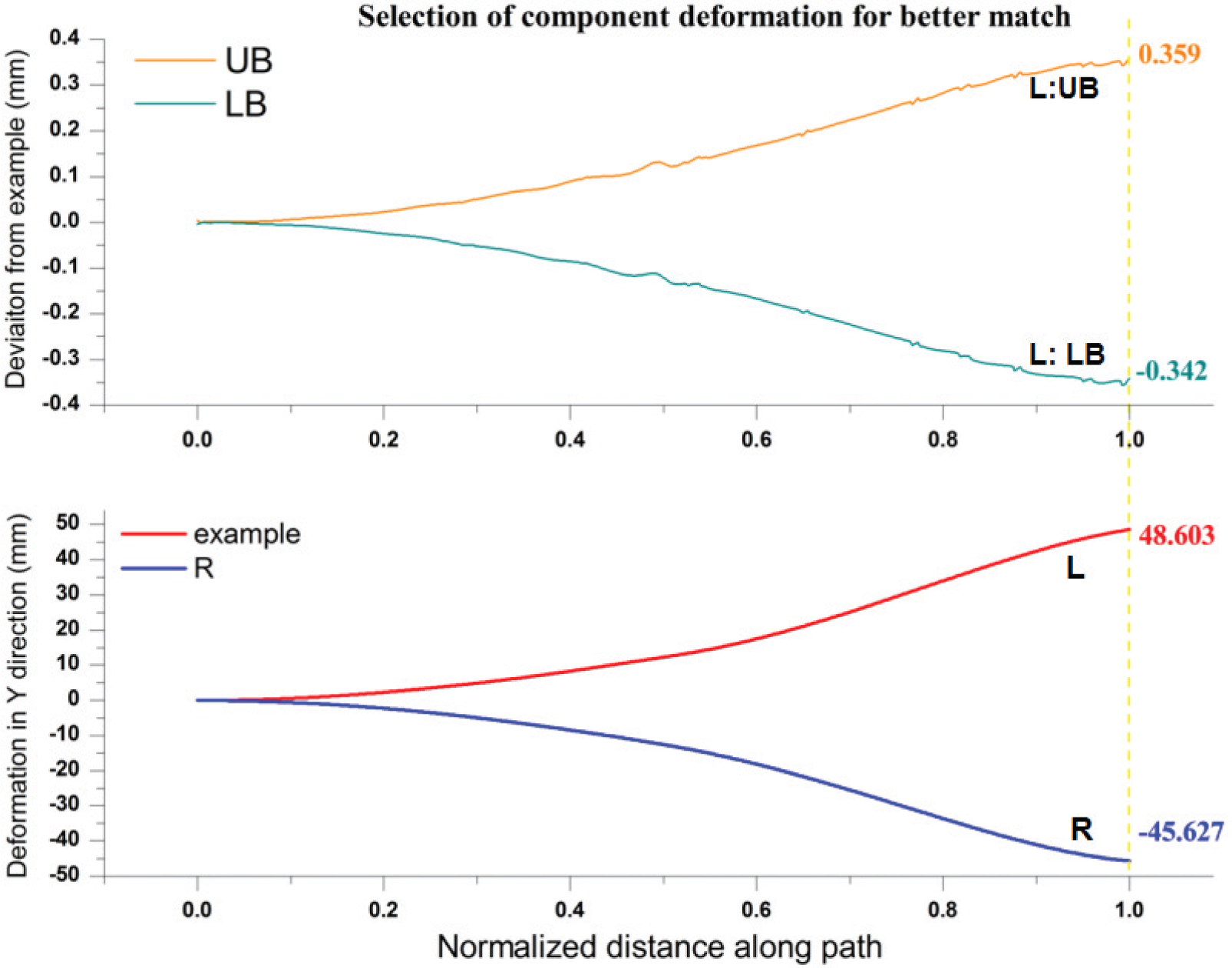
Selection of component deformation for better match-warping range.

In this matching case, Edge-R remains unchanged as baseline 3%. The changing values of weights corresponding to 10% stress component perturbation of Sxx-P2 and Sxx-P4 are −3.42 and 5.21, respectively (see Table 1). We check these relative differences from Figure 8 which lead to a 2.0% level closely. This means Edge-L should be manufactured from the material with 2.0% stretch ratio for better match with Edge-R which propagates from the material with 3.0% stretch ratio. It should be noted that the weights of Sxx-P2 and Sxx-P4 have certain relations under different processing conditions since they are the decomposition of the resultant stress profile. The optimized combination of stress weights obtained through downstream analysis could be fed back to the material processing as a demand for achieving that goal. Assembly variation concerning thick components thus can be controlled from the very beginning of manufacturing history chain, that is, the source of error from the material processing.

Discussion

• The developed method is mainly applicable to those typical assembly frame structures consisting of double long spars/edges and multiple webs/ribs. It can be implemented through adaption for similar structures such as trail edges of wing box and vertical stabilizer wing. Especially bulk residual stresses in these thick spars/edges’ raw materials dominate the large-scale deformation or warping in subsequent machining and assembly processes. The method is not suitable for thin-walled structures like panel assembly which is made up of thin skin and stringers. Multi-state riveting process affects panel assembly variation, and its variation propagation mode is also related to assembly datum or location mode, either from skin to stringer using pallet, or from stringer to skin using splint.^8,9 Thus, the applicable scenarios and the limitations of the methodology depend on the assembly structural characteristics. We highlight the major source of variation for frame assembly in our method, that is, thick main components. Assembly operations, like locating, clamping and joining, which also contribute to the assembly variation, can be further optimized based on the results of better match suggested by the developed method.

• The deformation’s amount fluctuates with the quality of different batches of blanks. If the bulk residual stresses remain at a lower range after material preparation, the component deformation induced by the release of residual stress will be smaller. If the blank’s state is not very good, the warping of edge will be much larger relatively. Additional straightening process is usually needed in such non-ideal situation, since plastic deformation during straightening might bring damage to the edge. This would also increase the cost and prolong the production cycle. The frame assembly we focus in the paper elicits the necessity of better match between two main edge components. This Edge-R’s state, that is, about 50 mm deformation and 50 MPa compressive surface stress, is verified in the field. We take it as trial center and study its better match Edge-L to illustrate the proposed methodology in which low stress state of blank should be guaranteed in the first place.

• The thick dominant edge in this case study is nearly 7 m long, and the resultant assembly deformation predictions shift from negative to positive several times as shown in Figure 11 or Figure 13. The relative positions of the ribs along path of normalized distance in the trailing edge assembly are indicated at the bottom of Figure 6. It can be seen that the rib’s positions correspond to the inflection points on the deformation curves, around which local minimum or maximum values and slope changes appear, like position 0, 40, 0.76, 0.95, 1.0. This result from internal stress redistribution/balance coupled with initial residual stress over the whole specific frame assembly after spring-back. The deformation trends (positive or negative values, steep or gentle slopes) depend on the structural characteristics of component and assembly. The edges are extremely long components with variable cross-section. The frame assembly of trailing edge is gradually constricted approaching its small end with various shapes of ribs mounted at different intervals. If these geometric features remain unchanged relatively, the patterns confined within specific ranges represented by normalized distance will not change. So, when it comes to the edge length change, these range locations will be different generally unless the uniform scale structural changes are made. If the ribs are kept the same (size and relative positions along path of normalized distance), the concerned range location will not differ a lot, for example, the negative concave deformation curve will still occur around range [0.2–0.4].

Conclusion

This article further investigates the impact of bulk residual stress in thick component originating from material preparation processing on large-scale assembly deformation, based on our previous study about basic analysis approach and its experiment validation in consideration of residual stress factor.

This study presents a quantitative variation propagation modeling method which can reflect the deformation situation concisely and its transition to enhance the understanding of overall variation impact induced by initial bulk stress fluctuation in raw materials. Legendre polynomials are used to represent non-linear stress perturbation patterns which further relate to stretch ratio as one of major material processing parameters, while Spline basis functions are capable of representing localized deformation pattern without loss of geometric covariance. An effective pattern mapping method is developed graphically between Legendre and Spline weight coefficients revealing the region of influence. A case study of the horizontal stabilizer assembly is presented to illustrate the proposed methods combined with orthogonal regression analysis using FEA aimed at better match. The methods are beneficial to quality control emphasizing a holistic view on residual stress factor and improve compliant assembly precision systematically in the following aspects:

• Predicting the overall deformation of multi-station assembly systems.

• Suggesting the practical main component selection for better match.

• Providing the basic framework for accumulating domain knowledge, experiment validation, field data and simulation results comprehensively.

• Providing the rational basis for launching manufacturing requirement from the standpoint of downstream assembly process considering upstream fabrication history.