Heat flux distribution and temperature prediction model for dry and wet cylindrical plunge grinding

Abstract

The grinding heat is generally partitioned into the workpiece, wheel, chips and fluid in grinding process. The total amount of heat flux entering into the workpiece greatly affects the final workpiece surface temperature, which may cause undesirable workpiece burn. Moreover, the variable grinding chip thickness and fluid injection speed along the grinding contact zone could substantially change the specific energy and the shape of the heat source correspondingly. In this article, a Weibull heat flux distribution model for both dry and wet grinding temperature prediction was proposed by analyzing two key parameters: energy partition R_w and shape parameter k. The value of R_w was obtained by considering the real contact length, the active grits number and the average grit radius r₀ on the basis of traditional formulas. The relationship between shape parameters k and useful flow was established by a FLUENT simulation of the convective grinding fluid applied in grinding contact zone with wheel-workpiece minimum clearance. The grinding temperature and grinding force experiments were conducted on a grinding machine MGKS1332/H to validate the proposed heat flux model. The calculated workpiece surface temperature distribution was obtained by using the experimental heat flux obtained by the reverse algorithm, and the error between calculated temperature and experimental temperature was analyzed. With the monitored force signals and the proposed temperature prediction model, the grinding temperature for both dry and wet grinding can be predicted, which will be helpful to the optimization and control of temperature in grinding process.

Introduction

Grinding is one of the most widely used precision machining methods, which is very effective and important for machining process. ¹ In grinding process, large amount of energy is expended to remove workpiece material, and unwanted heat in grinding can cause detrimental thermal damage which can lead to a reduction in component service life. ² Cooling is undoubtedly the most direct way to reduce the generated grinding heat away in the grinding zone and thus help to control the workpiece temperature and avoid the possible occurrence of thermal damage to the workpiece surface. When grinding fluid is injected into the grinding contact zone, it will fill in the pores between the wheel bond and the abrasive grits, reduce the grinding temperature and improve the life of the grinding wheel. ³

The grinding heat flux models were generally developed by coupling the heat transfer among grains, workpiece and coolant, in which the heat flux was assumed to be a solid moving at the wheel speed. ⁴ Most previous researches have concentrated on the energy partition to estimate the workpiece surface temperature, and the energy partition coefficient is usually obtained by matching the theoretical and experimentally determined temperatures in the grinding zone. ⁵ Finite element method (FEM) model has also been built for the analysis of grinding temperature field. ⁶ The heat flux to the workpiece is often assumed to conform to a uniform or triangular distribution. ⁷ A square law distribution has also been evaluated by Rowe et al. ⁸ and shown to give the best match between the measured and theoretical temperatures for the conventional shallow-cut conditions. Inverse heat transfer analysis has been investigated by Malkin and Guo ² to derive the grinding heat flux distribution from the measured temperature signals, by using the temperature matching, integral and sequential methods. For cylindrical dry grinding, Rayleigh distribution heat flux model was proposed ⁹ and verified to be a more accurate heat flux model in the contact arc length in cylindrical plunge grinding. However, the traditional heat flux model mostly focused on the influence of fluid on total energy partitioned into the workpiece, neglecting the influence of the shape of heat source on grinding temperature.

The air barrier surrounding the grinding wheel acts to restrict coolant access to the grinding zone. The useful fluid entering the grinding zone and crossing the interface would be decreased to 5%–40%. ¹⁰ Mihic et al. ¹¹ developed a numerical model based on computational fluid dynamics (CFD) to analyze fluid flow and thermal aspects in grinding and indicated that the useful flow rate is around 20%. Jin and colleagues^12,13 estimated of the convection heat transfer coefficient of coolant within the grinding zone and analyzed the grinding chip temperature and energy partitioning in high-efficiency deep grinding. Lavisse et al. ¹⁴ used an inverse matching method with a foil/workpiece thermocouple to determine the global heat flux distribution and energy partition in the workpiece when grinding under oil lubricant. Yin and Marinescu ¹⁵ a grinding process heat transfer model with various grinding fluid application is introduced based on CFD methodology. Zhang and colleagues ¹⁶ presented a new convective heat transfer model based on principles of applied fluid dynamics and found that heat transfer convection efficiency strongly depended on the grinding wheel speed, grinding arc length and fluid properties. Gviniashvili et al. ¹⁷ proposed a model of the useful flow rate and which is a function of the fluid acceleration power, grinding wheel speed and fluid jet velocity. The result showed that if the grinding fluid is not saturated, the different flow will lead to a change of heat source shape.

In this article, a temperature prediction model for dry and wet cylindrical plunge grinding was proposed based on Weibull heat flux distribution. Moreover, the key parameters of Weibull heat flux distribution model, k and R_w, were studied and the influence of fluid on both the amount and the shape of heat source was discussed in detail.

Temperature prediction model for cylindrical plunge grinding

Schematic description

The block diagram for the modeling concept of temperature prediction based on Weibull heat flux distribution is illustrated in Figure 1. It can be seen that the energy partition into the workpiece R_w and shape of the heat source k are calculated on the basis of process, material, wheel and fluid parameters. The heat transfer theory was used to predict the grinding temperature. If the heat flux entering into the workpiece q_w is a constant, the shape of the heat source k will be a crucial factor to the final workpiece temperature distribution.

Figure 1.

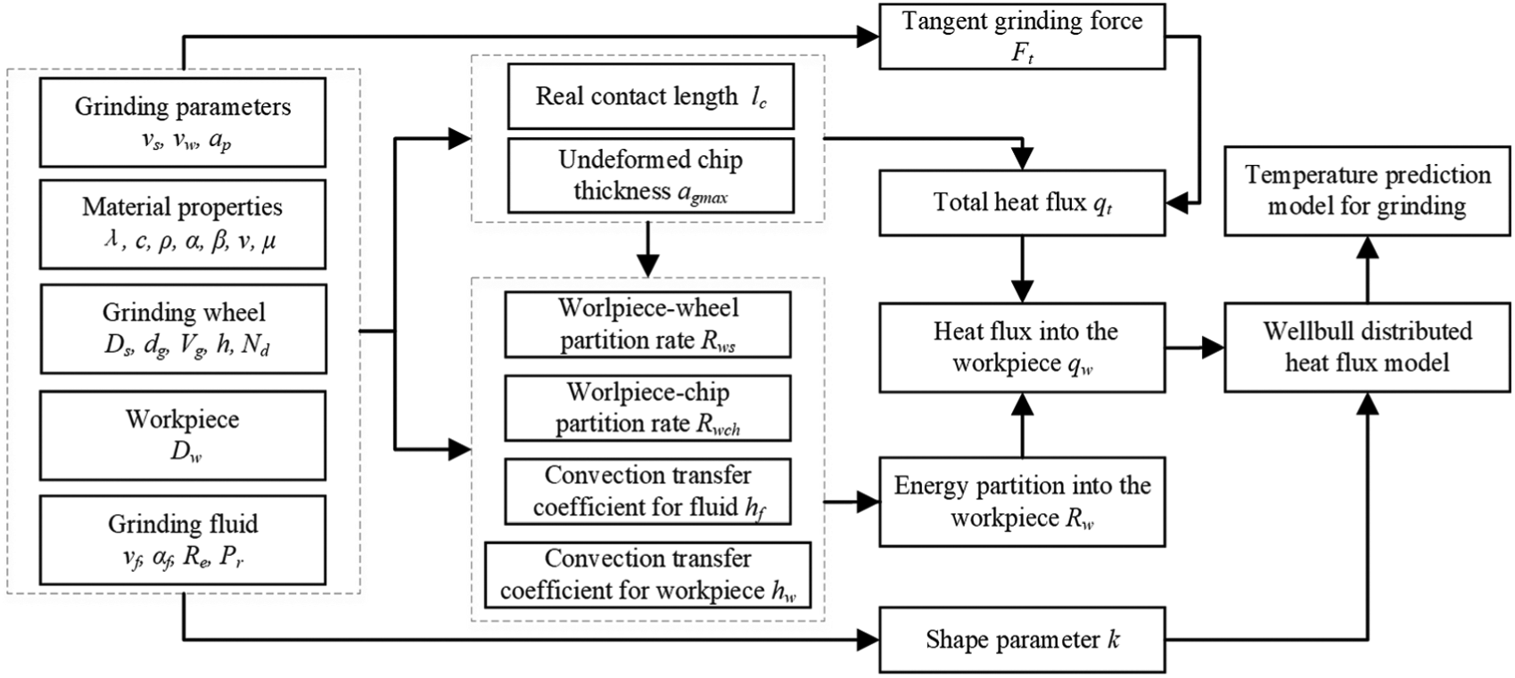
Temperature prediction model for cylindrical plunge grinding.

Weibull heat flux distribution

The heat transfer in grinding can be converted into the heat conduction in two dimensions, because the width of the grinding wheel b_s is much larger than the grinding depth a_p, and the workpiece speed is much lower than the grinding velocity. It is assumed the distribution of the heat flux q_w along the grinding zone is Weibull distribution as in equation (1) ¹⁸

$$f(x)=\{\begin{array}{cc}\frac{k}{\psi }{\left(\frac{x}{\psi }\right)}^{k-1}·e^{-{\left(\frac{x}{\psi }\right)}^k}\hfill & x\ge 0\hfill \\ \multicolumn{1}{c}{0}& x<0\hfill \end{array}$$

(1)

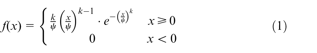
where k is the shape parameter, if k = 2, the Weibull distribution is identical to the Rayleigh distribution. $\psi$ is the scale parameter, which ensures the probability is more than 98% in the region of [0, 1].

The heat flux can be considered as an infinite heat flux with the heat flux density q(x) changing as a function of the position x. For a real grinding contact length l_r, q_w is defined as the heat flux transferred into the workpiece, as shown in Figure 2, which is moving along the surface of semi-infinite workpiece.

Figure 2.

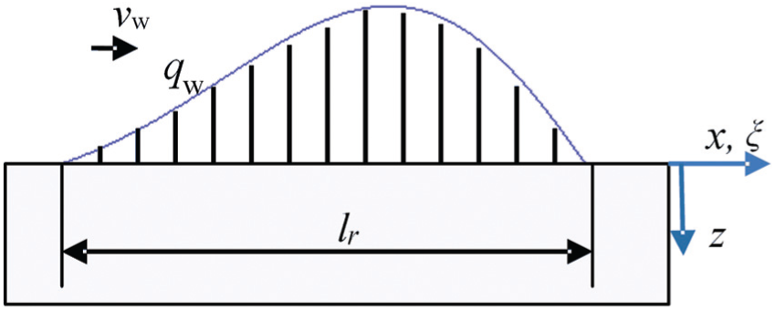
Heat flux distribution model. ⁹

Once the total heat flux to the workpiece is determined, the heat flux in the position x is given by a Weibull curve as equation (2)

$$q(x)=\frac{k}{\psi }{\left(\frac{x}{\psi ·l}\right)}^{k-1}·e^{-{\left(\frac{x}{\psi ·l}\right)}^k},0\le x\le l$$

(2)

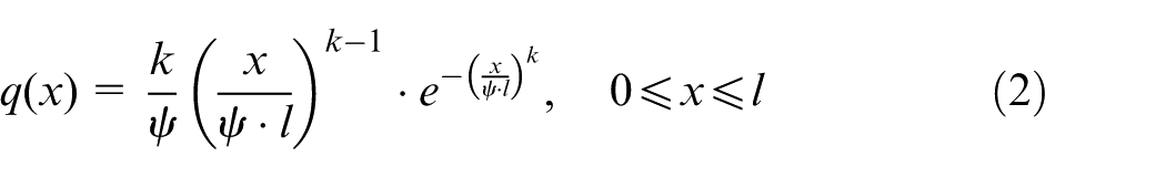
where l is the heat source length equal to the real contact arc length in the grinding contact area. The shape parameters k will affect not the total value but the distribution of heat flux into workpiece q_w, which will affect the final temperature distribution of grinding contact arc area on workpiece.

In the grinding zone, the integral of heat flux in the contact arc direction is the total heat flux into the workpiece

$$\underset{0}{\overset{l}{\int }}[\frac{k}{\psi }{\left(\frac{x}{\psi ·l}\right)}^{k-1}·e^{-{\left(\frac{x}{\psi ·l}\right)}^k}]\mathrm{dx}=q_{\mathrm{w}}·l$$

(3)

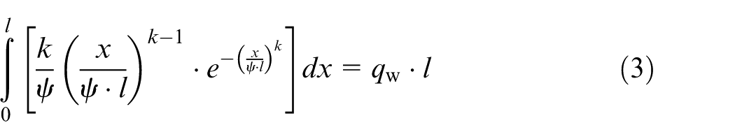
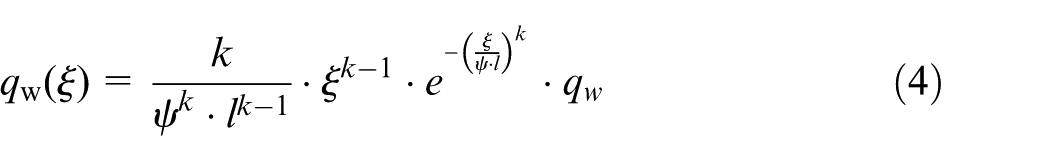
The total heat flux of the different heat flux model in the unit contact length is equal, so the heat flux equation of Weibull curve can be defined as in equation (4)

$$q_{\mathrm{w}}(\xi )=\frac{k}{{\psi }^k·l^{k-1}}·{\xi }^{k-1}·e^{-{\left(\frac{\xi }{\psi ·l}\right)}^k}·q_w$$

(4)

As shown in Figure 3, k = 2 represents the dry grinding, ⁹ and k > 2 represents the grinding with different cooling state. When the cooling fluid enters into the grinding contact zone, many parameters will affect the cooling effect of grinding fluid in the grinding zone, such as the wheel speed and the fluid speed. The total amount of the heat flux will be different and the shape of the heat source will be changed simultaneously. Different shape parameters k and different amount of q_w will affect the final workpiece surface and sub-surface temperature distribution.

Figure 3.

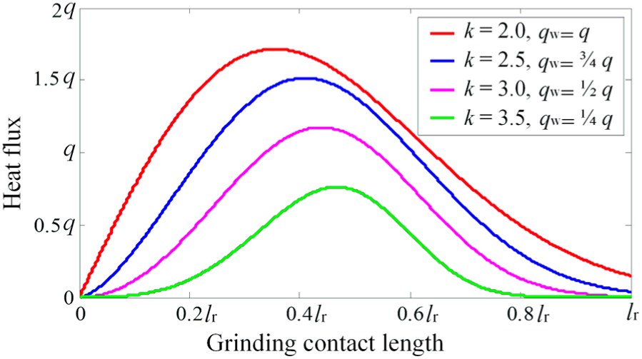
Weibull heat flux distribution model.

The temperature prediction model

The temperature distribution of the workpiece is described by Jaeger’s moving heat source model in equation (5)

$$\begin{array}{c}\multicolumn{1}{c}{T=\frac{k{q}_w}{\pi \lambda {\psi }^k{l}^{k-1}}\underset{0}{\overset{l}{\int }}{\xi }^{k-1}\exp [-{\left(\frac{\xi }{\psi l}\right)}^k-\frac{(x-\xi )v}{2\alpha }]}\\ K_0\left[\frac{v}{2\alpha }\sqrt{{(x-\xi )}^2+z_i^2}\right]d\xi \hfill \end{array}$$

(5)

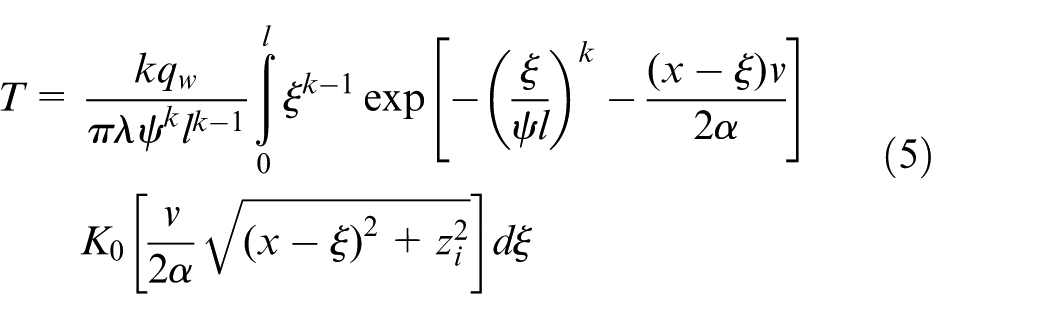
where K₀(x) is the modified Bessel equation of the second kind in zero order, λ is the thermal conductivity of the workpiece material, α is its thermal diffusivity, v_w is the moving velocity of the heat flux equals to the workpiece velocity and z_i is the sub-surface depth.

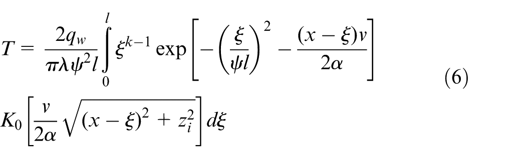
If k = 2, the temperature distribution of Rayleigh curve heat model is expressed as in equation (6)

$$\begin{array}{c}T=\frac{2q_w}{\pi \lambda {\psi }^{2}l}\underset{0}{\overset{l}{\int }}{\xi }^{k-1}\exp [-{\left(\frac{\xi }{\psi l}\right)}^2-\frac{(x-\xi )v}{2\alpha }]\hfill \\ K_0\left[\frac{v}{2\alpha }\sqrt{{(x-\xi )}^2+z_i^2}\right]d\xi \hfill \end{array}$$

(6)

If $u=x-\xi$ and $\mathrm{du}=-d\xi$ , equation (5) will be defined as in equation (7)

$$\begin{array}{c}T=\frac{-k{q}_w}{\pi \lambda {\psi }^k{l}^{k-1}}\underset{0}{\overset{l}{\int }}{(x-u)}^{k-1}\exp [-{\left(\frac{x-u}{\psi l}\right)}^k-\frac{\mathrm{uv}}{2\alpha }]\hfill \\ K_0\left[\frac{v}{2\alpha }\sqrt{u^2+z_i^2}\right]\mathrm{du}\hfill \end{array}$$

(7)

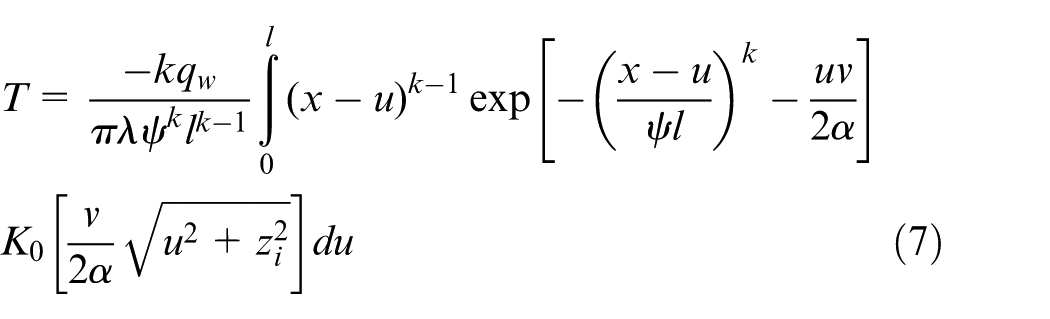
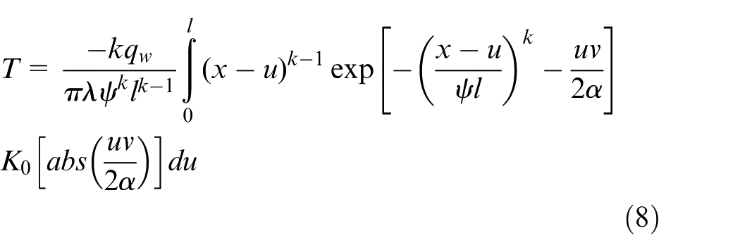
If z_i = 0, the temperature distribution of the surface of the grinding zone can be deduced as following

$$T=\frac{-k{q}_w}{\pi \lambda {\psi }^k{l}^{k-1}}\underset{0}{\overset{l}{\int }}{(x-u)}^{k-1}\exp \left[-{\left(\frac{x-u}{\psi l}\right)}^k-\frac{uv}{2\alpha }\right]K_0\left[abs\left(\frac{uv}{2\alpha }\right)\right]du$$

(8)

Heat transfer between wheel and workpiece

Grinding wheel topography

The wheel topography was modeled based on a diamond grinding wheel (99VG3A1-400-22-5 76 D91V+2046 J1SC-23 C150 E, WINTER). The wheel is 400 mm in diameter, 22 mm in width and 0.08 mm for average grit size d_g. By microscope observation, it can be found that the size, shape and distribution of grits on the grinding wheel surface are irregular. A circular truncated cone with the bottom diameter 80 µm is defined as the original grit, and different deformation will be added to every grit stochastically and the grit sizes will be different. The theoretical density can be defined by the distance S₁ and S₂ between grits. For grits locations, a cross-array arrangement of the grits is accomplished based on the average distance S₁ and S₂, as shown in Figure 4. The simulation of wheel surface topography is programmed by MATLAB to generate the corresponding surface abrasive grits distribution matrix. ¹⁹

Figure 4.

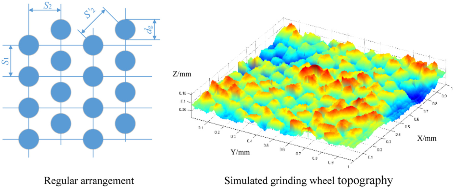
Original grit size, shapes and distribution for topography model.

Total heat flux q_t

The total heat flux q_t generated in grinding contact arc length can be expressed as equation (9), which can be solved by tangential grinding force, grinding wheel speed and grinding contact area. The grinding contract area is the real contact length multiplying the contact width between the wheel and the workpiece. The real contact arc length is much larger than the geometric contact length ⁸

$$q_t=\frac{P}{l_c·b_s}=\frac{F_t·v_s}{l_c·b_s}$$

(9)

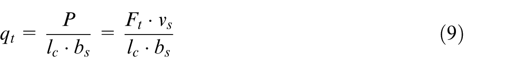
where b_s is the wheel width, v_s is the wheel speed, l_c is real contact arc length and F_t is the tangent grinding force.

The heat flux into the workpiece can be expressed as in equation (10)

$$q_w=q_t·R_w$$

(10)

where R_w is energy partition rate into the workpiece.

The energy partition into the workpiece R_w

Based on the Jin et al. model, ¹² the energy partition into the workpiece R_w can be calculated by equation (11)

$$R_w=\frac{1}{\frac{1}{R_{\mathrm{ws}}}+\frac{1}{R_{\mathrm{wch}}}-(1-\frac{h_f}{h_w})}$$

(11)

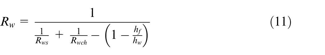
where R_ws is the workpiece-wheel partition rate, R_wch is the workpiece-chip partition rate, h_f is the convection heat transfer coefficient for fluid and h_w is convection heat transfer coefficient for workpiece.

Workpiece-wheel partition ratio, R_ws

Bases on the Hahn model and the transient function Black ²⁰ introduced, workpiece-wheel partition ratio, R_ws, in the steady state is defined as in equation (12)

$$R_{\mathrm{ws}}={(1+\frac{0.974·{\lambda }_g}{{\beta }_w·\sqrt{r_0·v_s}}·{(1-e^{-\frac{\sqrt{\frac{{\alpha }_g·l_c}{r_0^2·v_s}}}{2}})}^{-1})}^{-1}$$

(12)

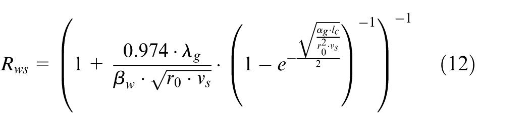
where r₀ represents an effective contact radius of the abrasive grits (mm) which is generally valued at from 0.005 to 0.01 mm, ¹³ λ_g is the thermal conductivity for grits, v_s is the wheel speed, ${\beta }_w=\sqrt{{\lambda }_w·{\rho }_w·c_w}$ is the thermal property parameters for workpiece, ${\rho }_w$ is the density for workpiece, ${\lambda }_w$ is the thermal conductivity for workpiece, $c_w$ is the specific heat capacity for workpiece and ${\alpha }_g$ is thermal diffusivity and calculated by ${\alpha }_g=\sqrt{{\lambda }_g/({\rho }_g·c_g)}$ . The thermal properties of the grinding wheel are required for energy partitioning in grinding. ²¹ The detailed physical properties of the diamond grits and workpiece are listed in Table 1.

Table 1.

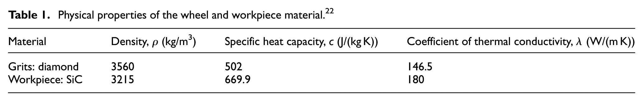
Physical properties of the wheel and workpiece material. ²²

Material	Density, ρ (kg/m3)	Specific heat capacity, c (J/(kg K))	Coefficient of thermal conductivity, λ (W/(m K))
Grits: diamond	3560	502	146.5
Workpiece: SiC	3215	669.9	180

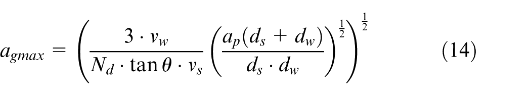
The grinding parameters, the actual contact arc length and the effective contact radius of the abrasive grits will affect the final results of R_ws. As shown in Figure 5(a), if v_s and a_p is fixed, R_ws will be changed with l_r and r₀. As the real contact arc length may be 1.5–2 longer than the geometry contact arc length in grinding, R_ws will be increased. If v_s, a_p and r₀ are fixed as 80 m/s, 0.008 mm/r and 0.01 mm, respectively, R_ws will be 0.48 for l_r = l_g and 0.56 for l_r = 2l_g. If v_s, a_p and l_r are fixed as 80 m/s, 0.008 mm and 2l_g, respectively, R_ws will be 0.57 for r₀ = 0.005 mm and 0.59 for r₀ = 0.01 mm. As shown in Figure 5(b), if r₀ and l_r is fixed, R_ws will be changed with v_s and a_p. If r₀, l_r and a_p are fixed as 0.005 mm, l_g and 0.008 mm, respectively, R_ws will be 0.49 for v_s = 40 m/s and 0.58 for v_s = 120 m/s. If r₀, l_r and a_p are fixed as 0.005 m, l_g and 0.02 mm/r, respectively, R_ws will be 0.48 for a_p = 40 m/s and 0.60 for a_p = 120 m/s. R_ws increases with the increase in wheel speed v_s and grinding depth a_p.

Figure 5.

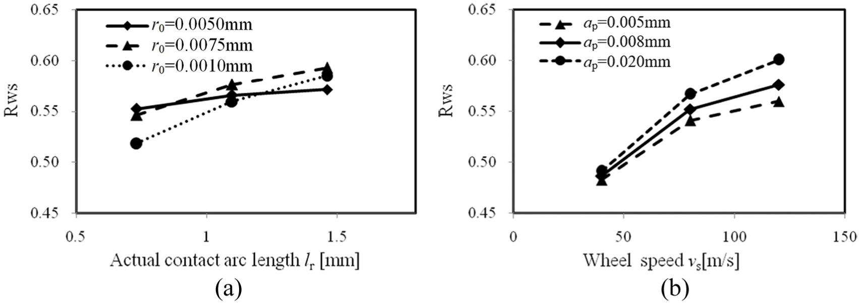
Calculated workpiece-wheel partition ratio: (a) v_s =80 m/s, a_p = 0.008 mm/r and (b) r₀ = 0.005 mm, l_r = l_g.

Workpiece-chip partition ratio, R_wch

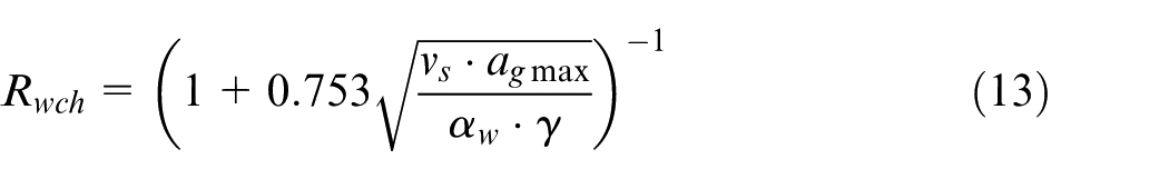
The workpiece-chip partition rate R_wch is expressed as in equation (13) ²³

$$R_{\mathrm{wch}}={(1+0.753\sqrt{\frac{v_s·a_{gmax}}{{\alpha }_w·\gamma }})}^{-1}$$

(13)

where ${\alpha }_w$ is the thermal diffusivity for workpiece, $\gamma$ is the shear strain and a_gmax is the undeformed chip thickness (mm). $\gamma$ can be calculated by $\gamma =\cos \theta /(\sin \phi \cos (\phi +\theta ))$ , $\theta$ is the half of grit tip angle, and $\phi$ is the shear angle, $\phi =({90}^{°}-\theta )/2$ . ¹³

The maximum undeformed chip thickness is defined as in equation (14) ²

$$a_{\mathrm{gmax}}={\left(\frac{3·v_w}{N_d·\tan \theta ·v_s}{\left(\frac{a_p(d_s+d_w)}{d_s·d_w}\right)}^{\frac{1}{2}}\right)}^{\frac{1}{2}}$$

(14)

where N_d is the active grits number per unit area, d_s is the wheel diameter, d_w is the workpiece diameter, v_w is the workpiece speed, a_p is the grinding depth and v_s is the wheel speed. The effective contact radius of the abrasive grits r₀ can be expressed as $r_0=a_{\mathrm{gmax}}·\tan \theta$ .

The grinding parameters and the active grits number will affect the final results of R_wch. As shown in Figure 6(a), R_wch decreases with the increase in v_s and v_w, while increases with the increase in a_p. If v_w and a_p are fixed as 0.1 m/s and 0.008 mm/r, respectively, R_wch is 0.70 for v_s = 40 m/s and 0.63 for v_s = 120 m/s. As shown in Figure 6(b), if v_s and v_w are fixed as 60 m/s and 0.1 m/s, respectively, R_wch increases with the increase in N_d, which is related to the grinding parameters.

Figure 6.

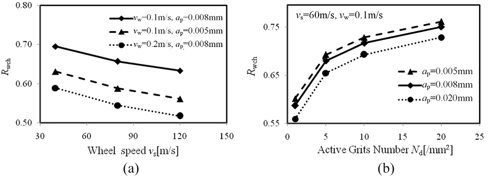
Calculated workpiece-chip partition ratio. (a) v_s VS. R_wch (b) N_d VS. R_wch.

Heat transfer coefficient for workpiece

Rowe et al. ⁸ proposed the convection heat transfer coefficient for workpiece

$$h_w=\frac{3}{2}·\frac{{\beta }_w}{C_1}·\sqrt{\frac{v_w}{l_c}}$$

(15)

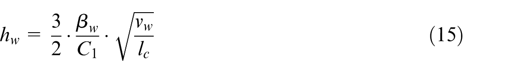
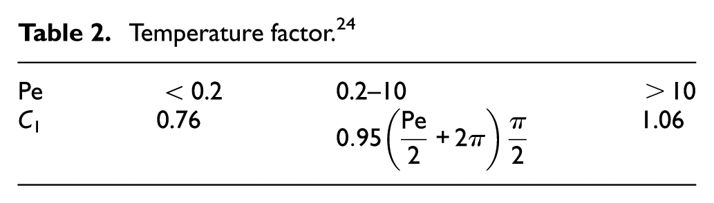
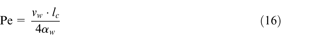
where C₁ is a temperature factor in Table 2, which changes with the Peclet number Pe

Table 2.

Temperature factor. ²⁴

Pe	<0.2	0.2–10	>10
C 1	0.76	$0.95(\frac{\mathrm{Pe}}{2}+2\pi )\frac{\pi }{2}$	1.06

$$\mathrm{Pe}=\frac{v_w·l_c}{4{\alpha }_w}$$

(16)

As shown in Figure 7, heat transfer coefficient for workpiece h_w is not a fixed value, which increases with the increase of v_w and decreases with the increase in the real contact arc length l_r.

Figure 7.

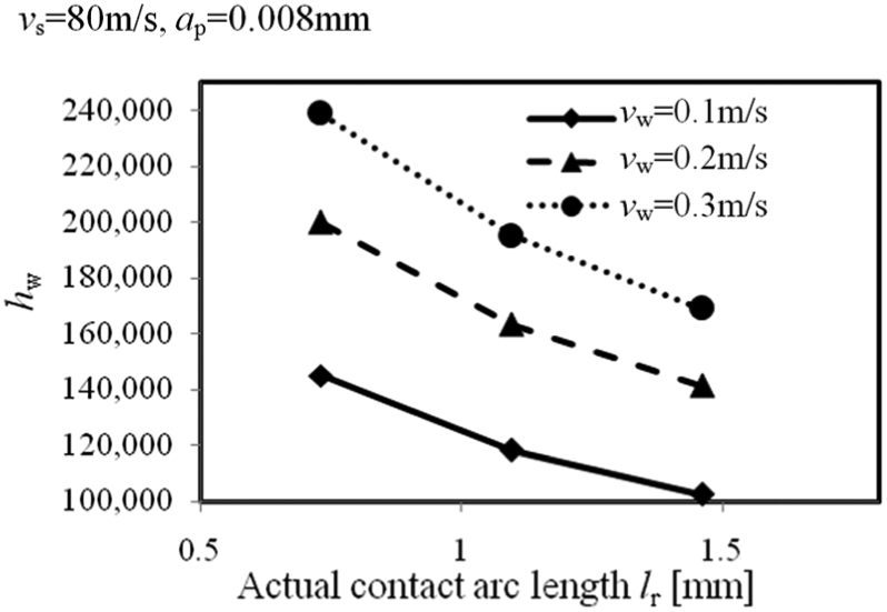
Calculated heat transfer coefficient for workpiece.

Heat transfer coefficient for fluid

The convection heat transfer coefficient for fluid is calculated by equation (17) ²⁵

$$h_f=\frac{\mathrm{N}{\mathrm{u}}_f·k_f}{d_g}$$

(17)

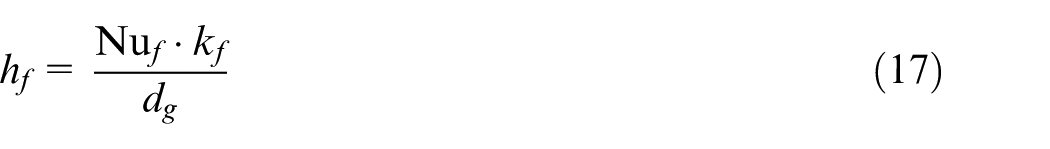
where d_g is the average grit size and k_f denotes the thermal conductivity of fluid. Nu _f is the Nusselt number calculated as $\mathrm{N}{\mathrm{u}}_f=1.04·{\mathrm{Re}}_f^{0.4}·\underset{f}{\overset{0.36}{⪻}}·(\underset{f}{⪻}/\underset{w}{⪻}{)}^{0.25}·{\epsilon }_n$ by Zhukauskas equation, ²⁶ Re _f is the Reynolds number for fluid as ${\mathrm{Re}}_f=(v_{\max }·L)/{\nu }_f$ and Pr _f is the Prandtl number for fluid as $\underset{f}{⪻}={\nu }_f/{\alpha }_f={\mu }_f/({\rho }_f·{\alpha }_f)=({\mu }_f·c_f)/k_f$ . Pr _w is the Prandtl number for workpiece. As the temperature varies considerably when the fluid enters the wheel surface, $(\underset{f}{⪻}/\underset{w}{⪻}{)}^{0.25}$ is used as a coefficient of physical correction.

In Figure 4, the static number of abrasive grits is 90/mm², S = S₁ = S₂ = 0.105 mm, d_g = 0.08 mm and $S{\prime }_2=(\sqrt{5}/2)S_1=117.4\mathrm{\mu }\mathrm{m}$ , $S{\prime }_2-d_g=117.4-80=37.4\mathrm{\mu }\mathrm{m}>(S_1-d_g)/2=12.5\mathrm{\mu }\mathrm{m}$ . According to the heat transfer of tube bundle, ²⁷ the maximum speed of fluid v_max is calculated as in equation (18)

$$v_{\max }=v_s\frac{S_1}{S_1-d_g}$$

(18)

As shown in Figure 8, heat transfer coefficient for fluid h_f is not a fixed value, which increases with the increase of v_f and decreases with the increase in distance between grits S.

Figure 8.

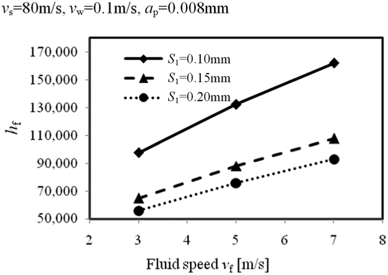
Calculated heat transfer coefficient for fluid.

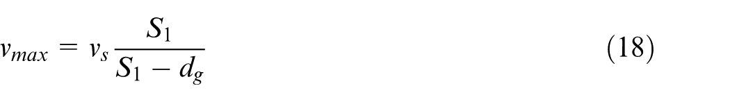
For the used grinding parameters, the corresponding R_w can be calculated by equation (11). The effect of grinding parameters and coolant changes on R_w is shown in Figure 9. v_f and a_p have a significant effect on R_w, while the effect of v_s on R_w is not obvious . R_w decreases with the increase of v_f, while increases with the increase of a_p.

Figure 9.

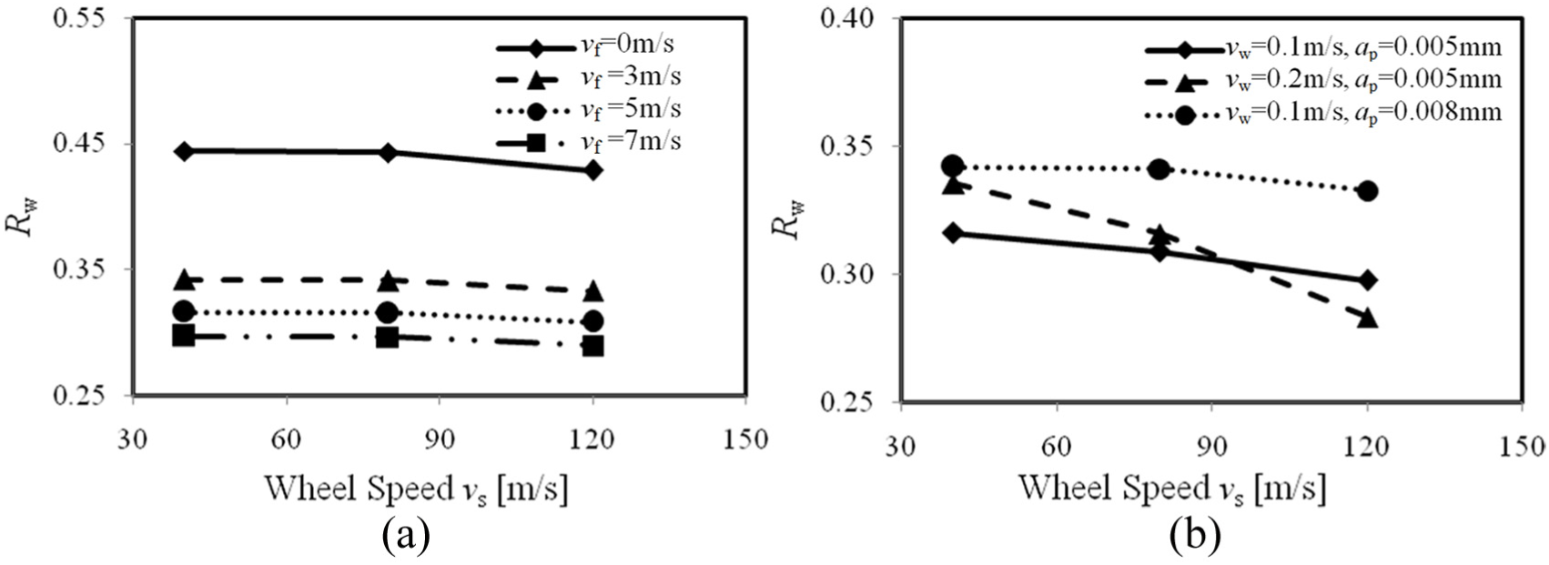
Calculated energy partition into the workpiece. (a) v_w =0.1 m/s, a_p = 0.008 mm and (b) v_f = 3 m/s.

Experimental setup

The experimental rig used for evaluating the grinding temperature is illustrated in Figure 10. The experiments were carried out on a high- speed CNC cylindrical grinding machine (MGKS1332/H, China). The workpiece used for this investigation was Reaction-Sintered Silicon Carbide (SiC) ceramics with Ø80 mm in diameter and 20 mm in width which is separated into two parts. ²⁸ The diamond grinding wheel of Ø400 mm in diameter and 22 mm in width was balanced to below 0.002 mm. The surface temperature measurement was carried out by K-type thermocouples designed and embedded into the workpiece. A special slot, with a thickness of 0.25 mm and width of 1.5 mm, was manufactured to embed the thermocouple. The thermocouple signals on the rotating workpiece are transmitted to the non-rotating data acquisition equipment by a collecting ring. The outer ring and the inner ring of the collecting ring are relatively rotated, in which the inner ring is connected with the workpiece and the outer is connected with the workbench. The grinding temperature was sampled by USB-9213 (NI) and the grinding force was sampled by a DAQ system (LMS). The grinding force could be monitored by a designed dynamometer which was equipped on the rear center of the grinding machine, as shown in Figure 10. A three-dimensional force sensor (Kistler 9347C, Switzerland) was modified to be mounted on the grinding machine as a dynamometer for on-line grinding force. A mixed grinding fluid injection system was used to ensure the coolant could be effectively entered into the grinding arc zone. 5% Emulsified oil (MOBIL CUT100) was used as the coolant for wet grinding.

Figure 10.

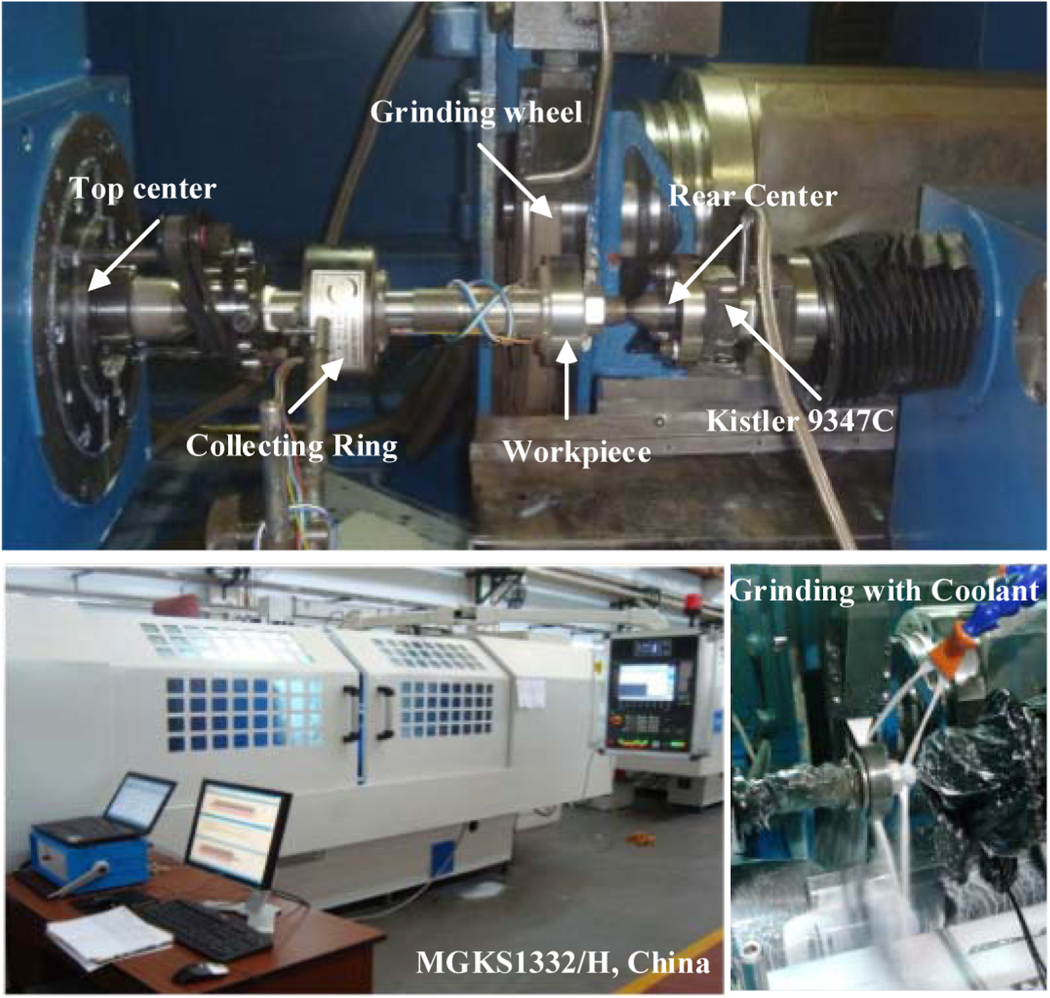
The experimental rig.

Determination of shape parameter k

Mean clearance between the grinding wheel and workpiece

Due to the high-speed rotation of the grinding wheel, the relative motion of the surrounding air will be changed, and the air barrier will be formed to prevent the grinding fluid entering into the contact area. The useful flow rate is defined as the proportion between the useful grinding fluid flow and nozzle flow, which is affected by the wheel speed, the coolant injection speed and the mean clearance between the grinding wheel and workpiece. ²⁹ According to the simulated wheel topography in Figure 4, the section curve of the wheel is shown in Figure 11.

Figure 11.

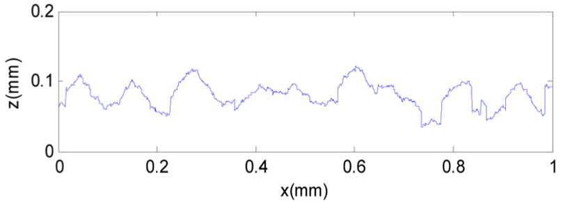
The section curve of the simulated wheel.

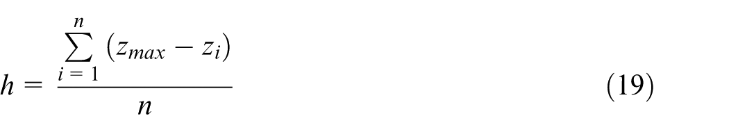
The mean clearance h could be defined as in equation (19)

$$h=\frac{\sum _{i=1}^n(z_{\max }-z_i)}{n}$$

(19)

Air barrier in high-speed grinding

The .msh files output by Gambit were imported into FLUENT. A collecting groove is set at the outlet of grinding zone as a straight line, which was at the exit of the grinding zone, as shown in Figure 12. The useful fluid flow of grinding zone under different parameters was calculated. After the iterative calculation for 1000 times, the distribution of the fluid flow field was obtained, as shown in Figure 12.

Figure 12.

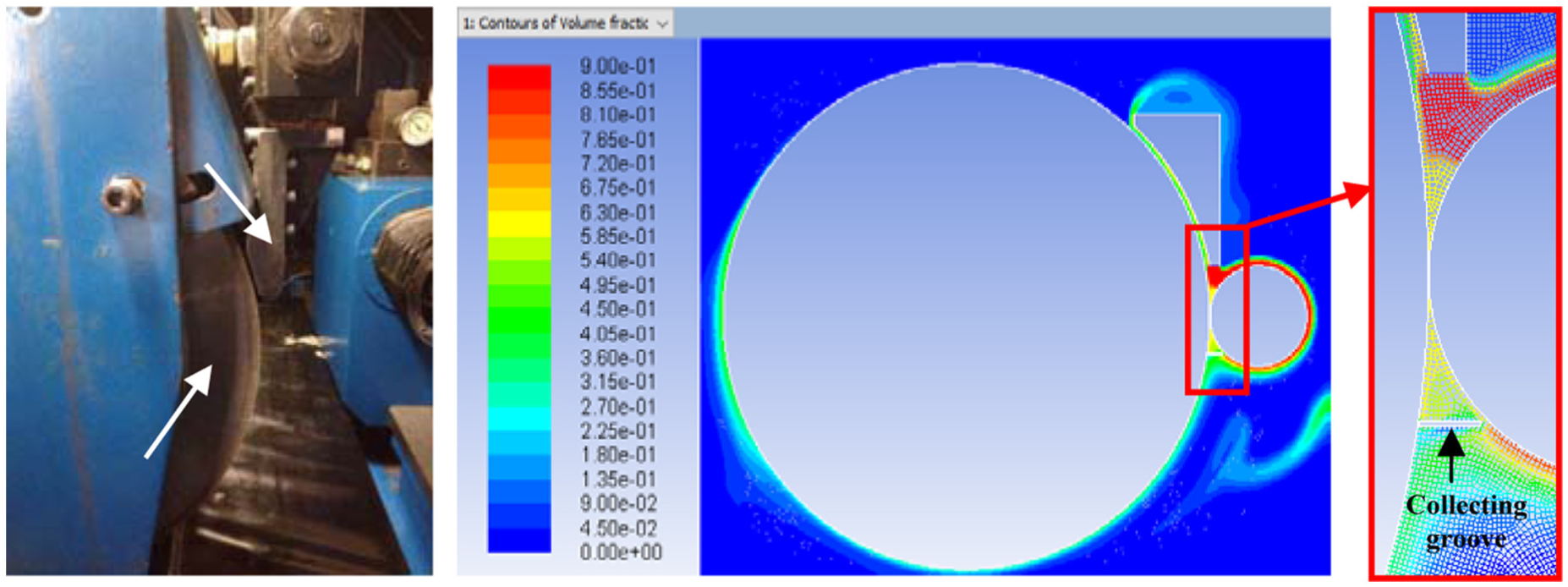
Profile of liquid distribution in grinding zone.

Based on the fluxes reports in FLUENT, the percentage of liquid flowing out of the outflow boundary can be calculated. In this model, the nozzle is the velocity output boundary and the collecting slot is the outflow boundary; therefore, the theoretical useful fluid flow rate can be obtained by calculating the ratio between them. The grinding wheel speed 40 m/s was used in the first simulation, and the grinding fluid velocity is 5 m/s. By the computation, the useful fluid flow rate is 42.7%. This data are only a theoretical useful flow rate, and there must be more grinding fluid which cannot enter the grinding zone in actual machining process. Moreover, in FLUENT simulation, the grinding fluid, which is back into the grinding zone, will also be considered as the useful flow rate, but this part of the grinding fluid is often not very good for cooling and lubrication. Therefore, the simulation results are only theoretical results and need further experimental verification.

Based on the previous analysis, it is found that the useful flow rate has a great relationship with the wheel speed and the fluid flow. The results of useful flow rate under different grinding parameters are solved by FLUENT simulation, and the results are shown in Figure 13. The greater the wheel speed, the lower the useful flow rate. It is because the greater the wheel speed is, the thicker the air barrier layer, the greater the return flow velocity is formed by the grinding wheel which seriously hinders the grinding fluid from entering the grinding zone. With the increase in jet velocity of grinding fluid, the useful flow rate will also increase. However, when the flow rate of the grinding fluid exceeds the minimum velocity, the effective flow rate will not increase or even decrease. Therefore, in order to increase the useful flow rate, it is not feasible to blindly increase the flow velocity of the grinding fluid.

Figure 13.

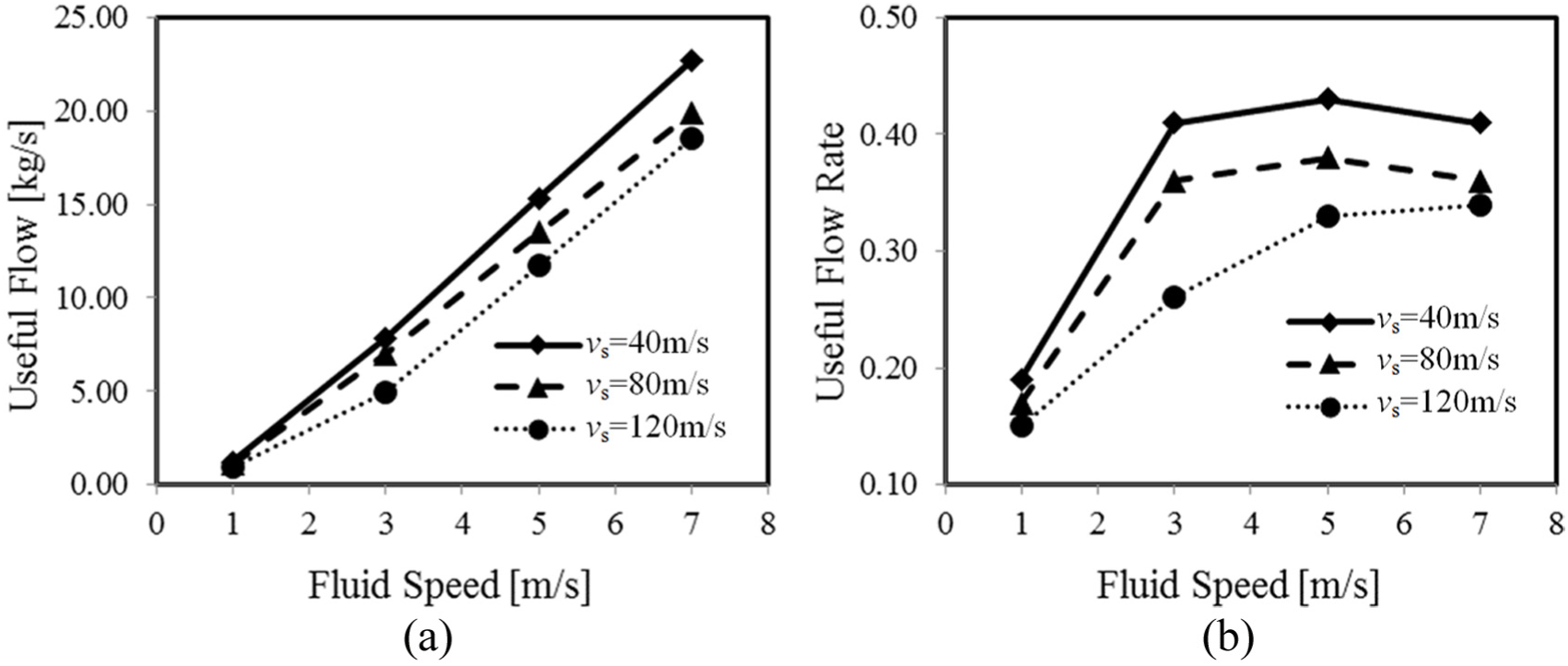
Useful flow and useful flow rate. (a) v_w =0.1 m/s, a_p = 0.008 mm and (b) v_w =0.1 m/s, a_p = 0.008 mm.

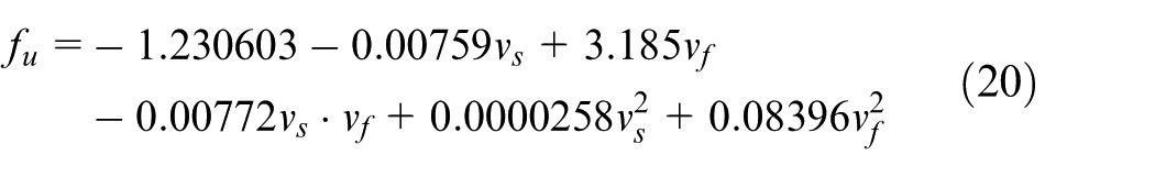
Based on the results of FLUENT simulation in Figure 13, the relations among the wheel speed (range from 20 to 140 m/s), fluid speed (range from 1 to 7 m/s) and the useful flow (range from 0 to 20 kg/s) were analyzed. With the tendency analysis of simulation data, the corresponding regressive equation for the useful flow can be established as in equation (20)

$$\begin{array}{c}\multicolumn{1}{c}{f_u=-1.230603-0.00759v_s+3.185v_f}\\ -0.00772v_s·v_f+0.0000258v_s^2+0.08396v_f^2\hfill \end{array}$$

(20)

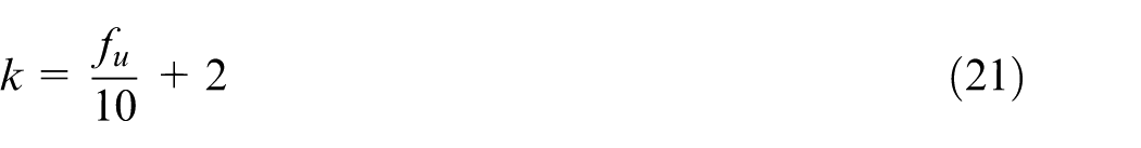
The useful flow is zero in dry cylindrical plunge grinding, and the shape parameter of heat flux entering into the workpiece k is 2. ⁹ It is defined that k is 4 for the useful flow 20 kg/s. 2 < k ≤ 4 represents shape of heat flux in the grinding with different cooling supply, which will affect the final workpiece surface and sub-surface temperature of workpiece. k and f_u are assumed to be linearly related, so the shape parameter k can be expressed as in equation (21)

$$k=\frac{f_u}{10}+2$$

(21)

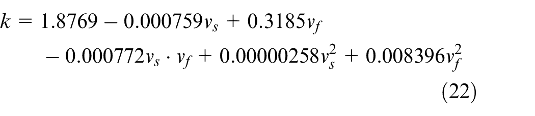
Substitute equation (20) into equation (21), k can be represented as follows (Figure 14)

$$\begin{array}{c}\multicolumn{1}{c}{k=1.8769-0.000759v_s+0.3185v_f}\\ -0.000772v_s·v_f+0.00000258v_s^2+0.008396v_f^2\hfill \end{array}$$

(22)

Figure 14.

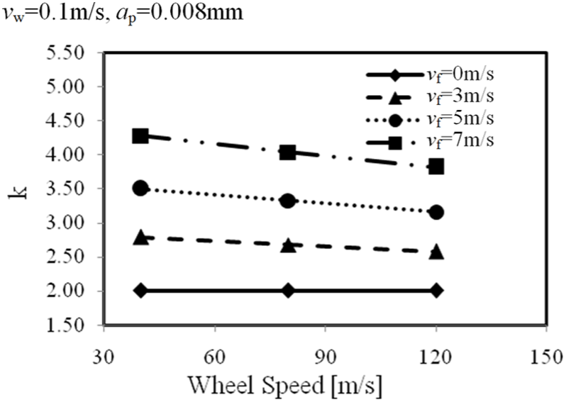
Calculated shape parameter for Weibull heat distribution.

Grinding heat flux and temperature

Experimental temperatures and heat flux

The grinding temperatures by experiments and the corresponding heat fluxes for dry and wet grinding with wheel speed 40 m/s is shown in Figure 15. The value of the wet grinding heat flux is obviously decreased to 45% of dry grinding with the effect of grinding fluid and the heat source shape was changed. The highest value of heat source moved toward the exit of the grinding contact arc zone. Substituting the values of the heat flux in Figure 15(b) and k calculated by equation (22), into equation (8), the calculated workpiece surface temperature distribution based on Weibull distribution heat flux model can be obtained as in Figure 15(c). For dry grinding, the experimental maximum temperature is 185.6 °C, while the calculated value is 172.3 °C, which means that the predicted error is 7.1%. For wet grinding, the experimental maximum temperature is 84.9 °C, while the calculated value is 81.5 °C, a 4.0% prediction error.

Figure 15.

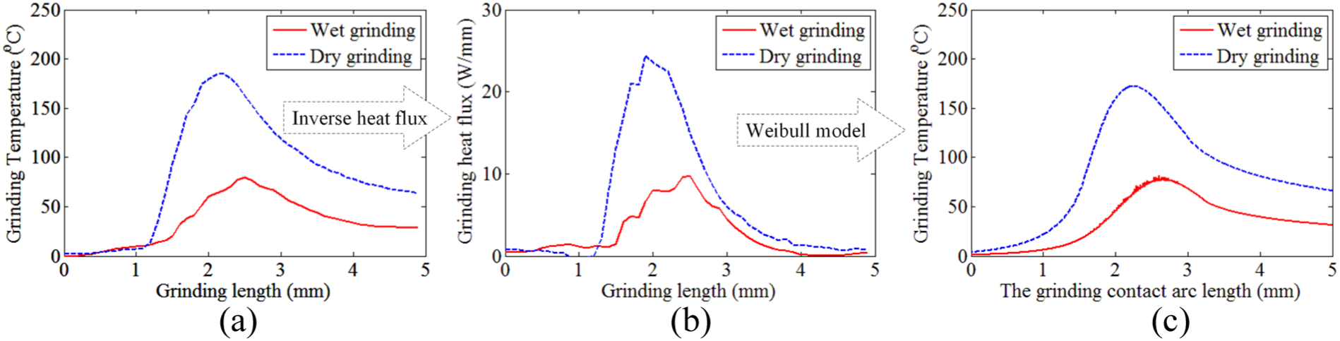
The workpiece surface and heat flux contrast between dry and wet grinding of 40 m/s (v_s = 40 m/s, v_w = 0.1 m/s, a_p = 0.008 mm/r). (a) Experimental temperature, (b) experimental heat flux and (c) temperature by Weibull model.

In Figure 16(a), the grinding with a speed of 120 m/s gets more obvious cooling effect after increasing fluid flow. Under the condition that the grinding fluid is not saturated, more grinding fluid can take away more grinding heat. The value of the heat flux is reduced to 80.05% by the same fluid rate as used in Figure 15(b), and the cooling effect reduces with the increase in the wheel speed. After increasing the flow rate by one time, the intensity of the heat source is reduced to 58.62%. The heat source of the front 1/2 arc in the grinding arc zone is reduced by cooling. Substituting the values of the heat flux in Figure 16(b), R_w and k calculated by equations (11) and (22), into equation (8), the calculated workpiece surface temperature distribution can be obtained as in Figure 16(c). For dry grinding, the experimental maximum temperature is 263.4 °C, while the calculated value is 260.0 °C, which means that the predicted error is 1.3%. For wet grinding (v_f), the experimental maximum temperature is 174.7 °C, while the calculated value is 200.4 °C, a 14.7% prediction error. For wet grinding (double v_f), the experimental maximum temperature is 140.4 °C, while the calculated value is 149.1 °C, a 6.2% prediction error.

Figure 16.

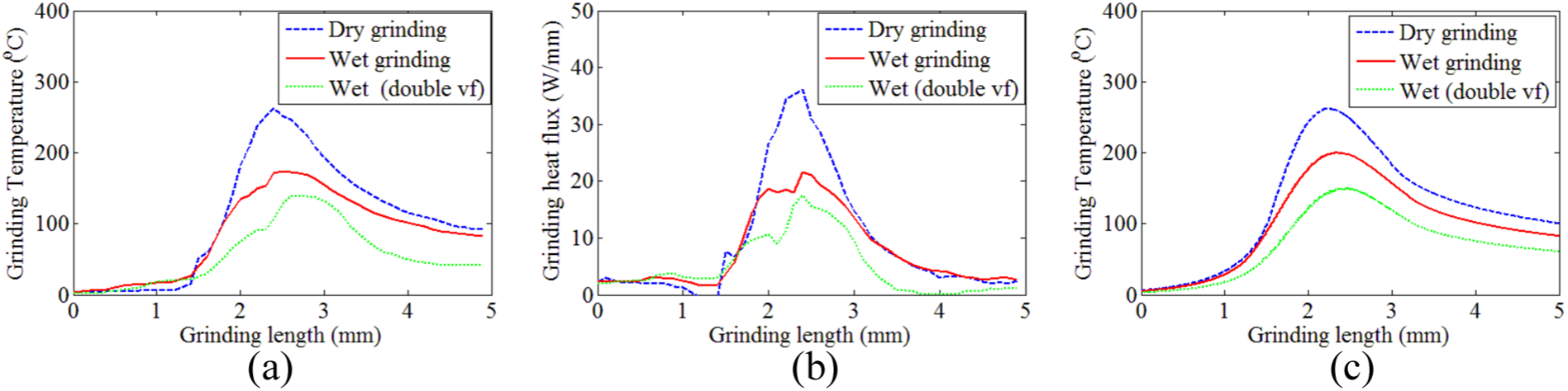
Temperature of the workpiece surface and thermal flow contrast between dry and wet grinding of 120 m/s (diamond grinding wheel, SiC workpiece, v_w = 0.1 m/s, a_p = 0.008 mm/r). (a) Experimental temperature, (b) experimental heat flux and (c) temperature by Weibull model.

Validation of the predicted grinding temperature

In grinding process, the measuring coordinate of the dynamometer relatively rotates to the coordinate of the grinding machine, and the measured tangential force would be periodic. In order to suppress the periodic load caused by the rotation of the workpiece spindle, a nipping fork was used. The nipping fork was connected to the driving lever by the flexible belt in order to avoid the unbalanced load. To evaluate and minimize the measure error, calibration of the dynamometer was carried out with a set of standard weights gradually and carefully loaded. With hardware filters, the raw force signals still contain a substantial amount of noise; 0–10 V voltage signals will be acquired by data acquisition system and be calibrated into the measuring force.

The raw and filtered force signals are shown in Figure 17. Before the contact between wheel and workpiece, the measured force had a periodic change due to the workpiece rotation. The grinding force increased immediately during grinding and decreased when the wheel left the workpiece. After the workpiece spindle stopped rotating, the measured force was changed into a constant. The normal and tangential force acting on the workpiece could be obtained. After 10 Hz low-pass digital filtering and signal amplifying and processing, the average value of the filtered force signals during the steady grinding period then will be employed as the experimental grinding forces.

Figure 17.

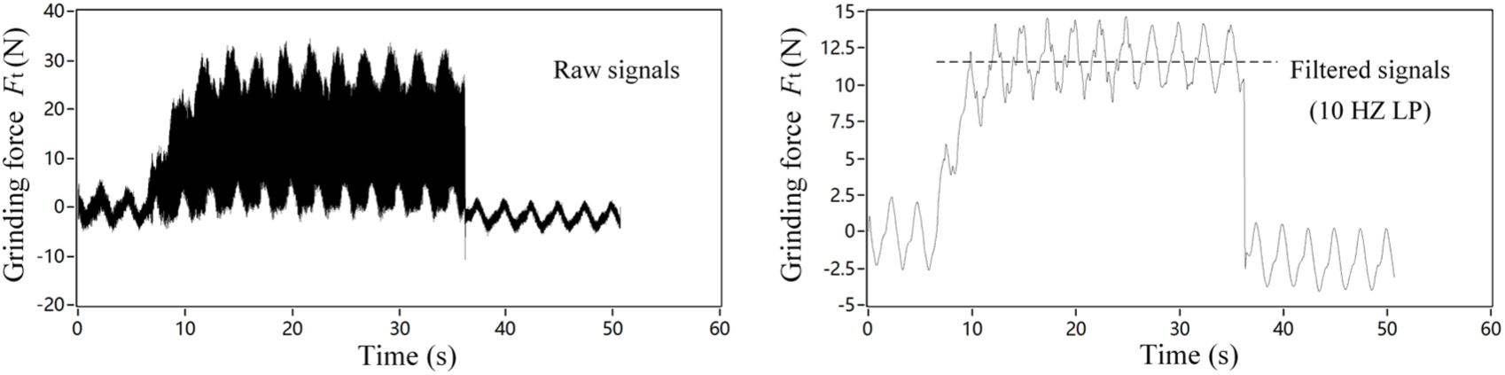
The monitored grinding force (v_s = 120 m/s, v_w = 0.1 m/s, a_p = 0.008 mm/r).

As shown in Figure 17, after the low-pass filter (10 Hz), the average grinding force was 11.62 N for the SiC dry grinding with wheel speed 120 m/s, workpiece 0.1 m/s and grinding depth 0.008 mm/r. Follow the proposed algorithm in Figure 1, the predicted grinding temperature distribution could be obtained with the monitored grinding force in Figure 17. As shown in Figure 18, the maximum rise of the predicted temperature was 262.3 °C, and the maximum temperature rise of the monitored temperature is 246 °C and 263 °C, respectively.

Figure 18.

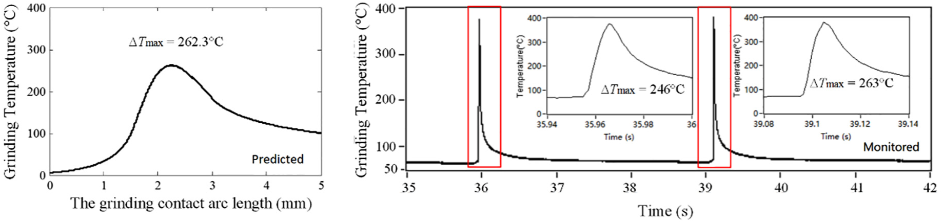
The predicted and monitored grinding temperature (v_s = 120 m/s, v_w = 0.1 m/s, a_p =0.008mm/r).

In order to further validate the proposed temperature model in both dry and wet grinding, a series of grinding experiments in Table 3 are conducted to investigate both the grinding force and temperature. It can be found that the predicted temperature value matches well with the experimental data, which has a low average predicted error of below 10%.

Table 3.

The monitored grinding force and predicted maximum temperature rise.

No.	vs (m/s)	vw (m/s)	ap (mm)	Coolant	Rws	Rwch	Rw	$F{\prime }_t$ (N/mm)	qt (W/mm2)	qw (W/mm2)	k	ΔTmax Weibull model (°C)	ΔTmax experiments (°C)	Error (%)
1	20	0.1	0.008	N	0.41	0.73	0.35	2.28	56.68	20.00	1.86	147.7	135.3	8.3
2	60	0.1	0.008	N	0.53	0.67	0.42	1.24	92.93	39.02	1.84	286.5	248.1	13.2
3	100	0.1	0.008	N	0.57	0.64	0.43	0.71	88.75	38.37	1.83	280.5	278.9	0.7
4	140	0.1	0.008	N	0.59	0.62	0.43	0.57	99.32	42.95	1.82	313.1	271.7	13.4
5	20	0.1	0.008	Y	0.41	0.73	0.28	1.29	32.00	9.04	2.85	75.3	79.0	4.9
6	60	0.1	0.008	Y	0.53	0.67	0.32	0.83	61.90	20.04	2.73	165.6	171.3	3.4
7	100	0.1	0.008	Y	0.57	0.64	0.33	0.69	85.36	28.27	2.63	231.3	233.2	0.9
8	140	0.1	0.008	Y	0.59	0.62	0.33	0.53	92.19	30.54	2.53	245.9	226.0	8.1

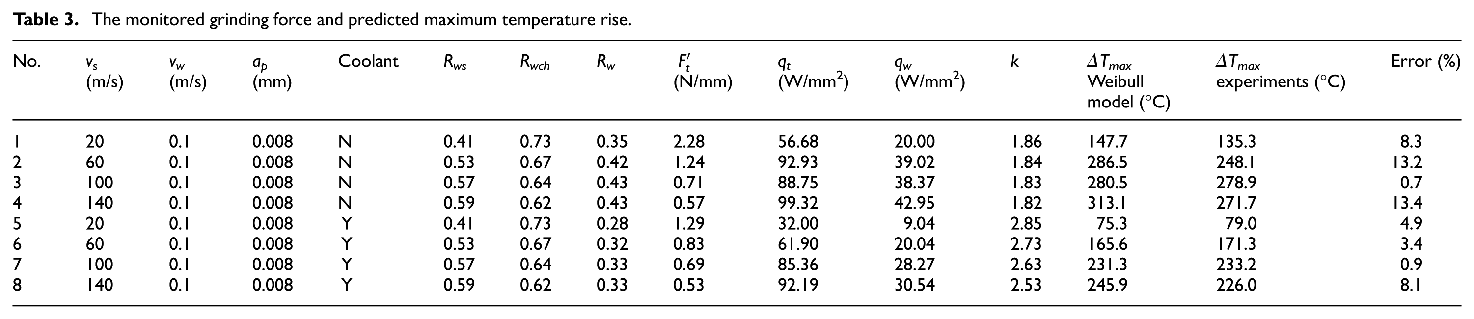
Figure 19 gives more concrete description of the prediction results with bar chart. It can be found that the grinding temperature increases substantially with the increase in grinding wheel speed to 60 m/s in both dry and wet grinding. However, when the grinding speed reaches up to 60 m/s, the grinding temperature slightly increases. While the grinding wheel speed is 100 and 140 m/s, the grinding temperature keeps relatively stable. In order to explain this phenomenon, one of the reasons could be attributed to a higher impact effect of grit-workpiece interaction under a higher wheel speed, which could help to increase the grinding temperature. On the other hand, the increase in wheel speed helps to increase the heat partition into workpiece R_w, while the heat partition into the wheel R_ws and chips R_wch decreases, which could be found in Table 3. The increase in wheel speed increases the interaction of the grits and the formation frequency of chips, which helps to reduce the wheel temperature and more produced chips take away the generated heat. That is why the grinding temperature could be suppressed in a high-speed grinding. Finally, it could be found that the wet grinding could help to reduce more grinding heat in low-speed grinding that was in high-speed grinding. This is because a stronger air barrier in high-speed grinding happens and more frequent grit–workpiece interaction makes the grinding process a more consecutive machining process, which makes the grinding heat conserved in the contact area. However, the air barrier problem could be alleviated through equation (20) in section “Air barrier in high-speed grinding.”

Figure 19.

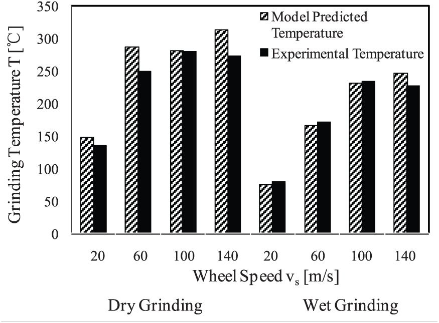
Validation of the predicted temperature model.

Conclusion

A heat flux model for both dry and wet grinding based on two key parameters, energy partition R_w and shape parameter k, was proposed in this article. R_w was derived by considering the real contact length, active grit number and the effective contact radius of the abrasive grits. The shape parameters k was deduced by the useful fluid, which will influence the shape of the heat flux into the workpiece. Grinding temperature experiments were carried out to verify the accuracy of the proposed Weibull distribution heat flux model, which shows a good match of about 10% prediction error. By using the reverse algorithm, the actual heat fluxes in different grinding parameters and different cooling conditions were obtained by experiments. Then, the proposed Weibull heat flux model was used to predict the temperature distribution using the monitored grinding force, and it was found that the proposed model is helpful to the optimization and control of temperature in grinding process. Through the grinding experiments, it could be found that the grinding temperature increases substantially with the increase in grinding wheel speed to 60 m/s in both dry and wet grinding. However, when the grinding speed reaches up to 60 m/s, the grinding temperature slightly increases. While the grinding wheel speed is 100 and 140 m/s, the grinding temperature keeps relatively stable. Moreover, the wet grinding could help to reduce more grinding heat in low-speed grinding that was in high-speed grinding.