Acceleration smoothing algorithm for global motion in high-speed machining

Abstract

When machining a series of short linear segments, the computer numerical control system interpolates the machining path with the pre-specified spline curve to obtain continuous feed motion. However, to obtain adequate smooth tool-paths to smooth the feed velocity and acceleration, the computer-aided manufacturing system needs to use a higher order spline curve, which will be limited by some technical bottlenecks. In this article, a new real-time interpolation algorithm is proposed from the perspective of kinematics to achieve uninterrupted feed motion throughout the global tool-path. At the same time, the acceleration profile achieves G² continuous to avoid unnecessary feed frustration and inertial impact, reaching the balance between time-optimal and motion performance. First, the jounce-limited acceleration curve is blended at the corner of the machining path, and the optimal cornering transition velocity is obtained by adding the velocity, acceleration and contour error constraints to the corner transition motion. Then, according to the linear segments with different lengths between the corners, combined with the feed motion around the corner, a look-ahead interpolation algorithm is proposed to calculate the maximum feed rate with the constraint of the linear segment length and kinematic boundary conditions. At last, for the linear segments whose corner contours overlap with each other after interpolation, the smooth transition between the two corners can be realized by mixing the feed motion of the next corner. Compared with non-uniform rational B-spline interpolation algorithm, the proposed algorithm reduces the total machining time by 14% and the computer numerical control system improves the computational efficiency by 11%. It proves that the proposed algorithm has better application value in the manufacturing of complex parts.

Introduction

In the aerospace, mold manufacturing and other fields, some complex contours of parts are often required. The computer-aided manufacturing (CAM) system usually discrete parts contour path into a series of consecutive linear segments, and discretization becomes finer and denser with the increasing of path curvature. During the machining process, the feed motion controlled by the CNC system must be stopped completely at the corner formed by the intersection of two short linear segments. This feed motion is called point-to-point (P2P) motion. In order to improve machining efficiency, forming a consecutive feed motion at the corner of the tool-path has become a widely used method.^1,2 The smooth high-order spline curve is interpolated around the sharp corner and the feed planning is carried out in the mixed linear segments at a higher tangential speed for better machining quality. However, the interpolation of the high-order parameter curve deviates from the original machining path to form the contour error. ³ This is not always detrimental. If the contour error is controlled within a certain range, this method can be applied to roughing or semi-finishing, which can greatly improve the machining efficiency. Many experts and scholars have proposed a variety of spline curve interpolation methods to control the contour error.^4–9 Zhao et al. ⁵ used the B-spline curve to fit the selected dominant points, generating the smooth tool-path and federate profile. Lu et al. ⁶ used the cubic B-spline curve interpolation path and applied the iterative optimization process to obtain the knot vector element, attaining high accuracy and computation efficiency. Han and Chen ⁷ proposed the new velocity control algorithm to limit velocity fluctuations and to achieve a controllable jerk value based on the non-uniform rational B-spline (NURBS). Zhang et al. ⁸ proposed the equidistant double NURBS interpolation algorithm to obtain uninterrupted feed motion and further improve the machining accuracy. After the local corners are smoothed, the reasonable motion planning is performed on the mixed linear segments. S-type acceleration and deceleration based on jerk-limited acceleration^5,6 are widely used in high-speed motion, generating the smooth velocity profile by piecewise constant jerk segments, providing the balance between the smoothness of the machined surface and the optimal time. ¹⁰ However, this two-step uninterrupted feeding strategy is inefficient and complicated. In general, the curve interpolation between the corners is the high-order parameter curve, which is limited by some real-time interpolation bottlenecks, such as the inability to accurately calculate the curve lengths, the inability to effectively suppress the chord error and the inability to accurately control the contour error.^11–13 Therefore, some scholars recently started to explore the method of directly completing the uninterrupted feed motion in one step and generating a smooth machining path and velocity profile. Tsai and Huang ¹⁴ proposed a dynamic acceleration and deceleration interpolation algorithm by adding the finite impulse response (FIR) filters to achieve the smooth transition velocity. Tajima and Sencer ¹⁵ proposed the kinematic corner smoothing technique to achieve corner smooth transitions with optimal time. Biagiotti and Melchiorri ¹⁶ used the FIR filter to generate minimized machining time under the constraints of velocity and acceleration. Fan et al. ¹⁷ developed an efficient convex optimization method to address the time-optimal feed rate planning problem with these complex constraints. However, the current algorithms mainly realize the technology of uninterrupted feed motion by smoothing the corners and assume that the linear segment between corners is long enough for the driver to achieve local corner smoothing. There are relatively few studies on the uninterrupted feed motion with short linear segments between corners and even overlapping corner profiles. The acceleration curve with G¹ continuous has non-conductive points, which will cause additional inertial vibration and impact. Therefore, a new real-time interpolation method based on kinematics is proposed in this article; the consecutive feed motion strategy is implemented in the global machining path and generates G² continuous acceleration curve. First, the jounce-limited acceleration curve is mixed with the feed speed and acceleration of the axis to generate the corner’s uninterrupted feed motion. Considering the kinematic profiles of the corners and the length of the linear segments between the corners, the look-ahead interpolation algorithm is proposed to achieve the optimal time in the feed motion between corners. At the same time, for the linear segments where corner profiles overlap each other, the kinematic profiles at the corners are taken into consideration, and the contour path of the next corner is mixed to generate the smooth feed motion. Simulation and experimental results show that the algorithm can generate the tool-path with the specified contour error along the short linear segments, and the acceleration reaches G² continuous.

Uninterrupted cornering motions with smoothed acceleration

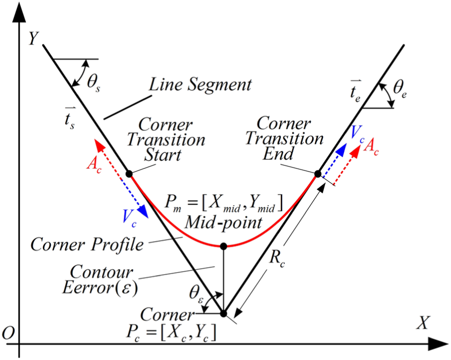
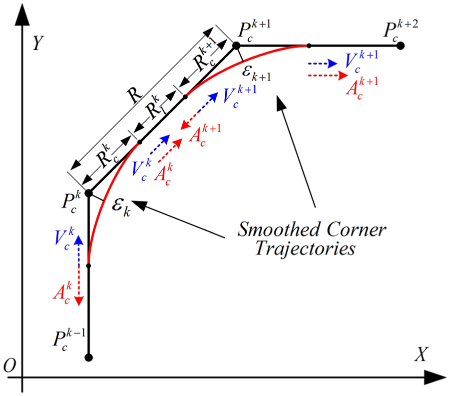
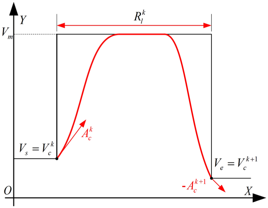
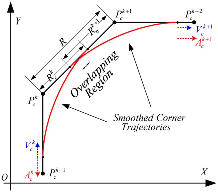
In this section, the velocity and acceleration are planned directly around the corners based on the jounce-limited acceleration curve to generate the smooth corner profile trajectory, as shown in Figure 1. The two linear segments t_s and t_e intersect to form the corner point P_c whose Cartesian coordinate position is [X_c,Y_c] and the direction of the linear segment is θ _s and θ _e . In order to realize the uninterrupted feed motion, it is assumed that the corner motion starts and ends with the same velocity V_c and acceleration A_c so that the corner contour can be obtained symmetrically around the corner bisector. The corner bisector divides the corner contour into two sections, the duration of the previous period is T₁, the duration of the latter period is T₂, and the total cornering duration is T₁ + T₂ = T_c. The maximum contour error is at the midpoint of the corner contour. The Euclidean distance from the beginning and end of the cornering transition to the corner point P_c is R_c. Based on the above conditions, the kinematic curves can be derived by integrating the jounce curve, and the maximum transition velocity, the cornering duration and the corresponding jounce value are further deduced.

Figure 1.

Corner interpolation algorithm.

The kinematic curves are shown in Figure 2. At the corner of the path, the feed velocity is controlled by the piecewise constant jounce segments to ensure uninterrupted feed motion; thus, the smooth acceleration curve is formed to achieve the optimal feed strategy. For X–Y plane motion, kinematic profiles in Figure 2 are

$$\{\begin{array}{l}{s}_x(\tau )=\{\begin{array}{l}{S}_x,0\le t<t_1\\ -S_x,t_1\le t<t_2\end{array}\\ j_x(\tau )=\{\begin{array}{l}{S}_x{\tau }_1,0\le t<t_1\\ -S_x{\tau }_2+S_x{T}_1,t_1\le t<t_2\end{array}\\ a_x(\tau )=\{\begin{array}{l}{A}_{sx}+\frac{1}{2}{S}_x{\tau }_1^2,0\le t<t_1,A_{1x}=A_{sx}+\frac{1}{2}{S}_x{T}_1^2\\ A_{1x}-\frac{1}{2}{S}_x{\tau }_2^2+S_x{T}_1{\tau }_2,t_1\le t<t_2,A_{ex}=A_{1x}-\frac{1}{2}{S}_x{T}_2^2+S_x{T}_1{T}_2\end{array}\\ v_x(\tau )=\{\begin{array}{l}{V}_{sx}+A_{sx}{\tau }_1+\frac{1}{6}{S}_x{\tau }_1^3,0\le t<t_1,V_{1x}=V_{sx}+A_{sx}{T}_1+\frac{1}{6}{S}_x{T}_1^3\\ V_{1x}+A_{1x}{\tau }_2-\frac{1}{6}{S}_x{\tau }_2^3+\frac{1}{2}{S}_x{T}_1{\tau }_2^2,t_1\le t<t_2,V_{ex}=V_{1x}+A_{1x}{T}_2-\frac{1}{6}{S}_x{T}_2^3+\frac{1}{2}{S}_x{T}_1{T}_2^2\end{array}\\ r_x(\tau )=\{\begin{array}{l}{R}_{sx}+V_{sx}{\tau }_1+\frac{1}{2}{A}_{sx}{\tau }_1^2+\frac{1}{24}{S}_x{\tau }_1^4,0\le t<t_1,R_{1x}=R_{sx}+V_{sx}{T}_1+\frac{1}{2}{A}_{sx}{T}_1^2+\frac{1}{24}{S}_x{T}_1^4\\ R_{1x}+V_{1x}{\tau }_2+\frac{1}{2}{A}_{1x}{\tau }_2^2-\frac{1}{24}{S}_x{\tau }_2^4+\frac{1}{6}{S}_x{T}_1{\tau }_2^3,t_1\le t<t_2,R_{ex}=R_{1x}+V_{1x}{T}_2+\frac{1}{2}{A}_{1x}{T}_2^2-\frac{1}{24}{S}_x{T}_2^4\\ +\frac{1}{6}{S}_x{T}_1{T}_2^3\end{array}\end{array}$$

(1)

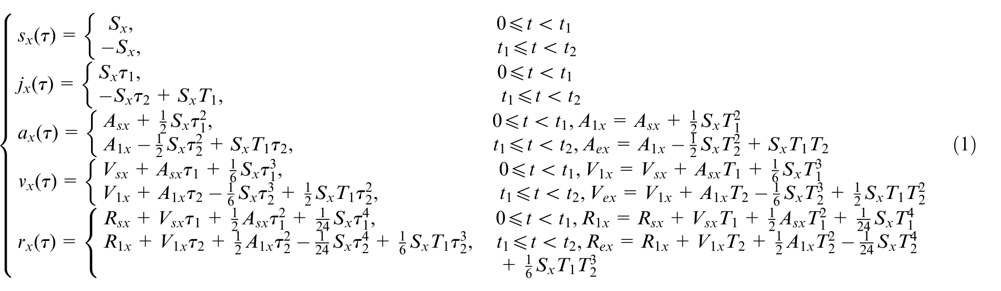
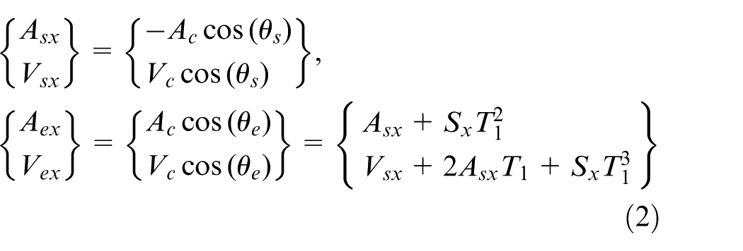
where t is the cornering time, T₁ = T₂=T_c/2, and S_x is the jounce magnitude. The Y-axis equations need to replace the x to y. The boundary conditions of velocity at the beginning and end of the corner motion are V_s and V_e, and the acceleration boundary conditions at the beginning and end of the corner motion are A_s and A_e which can be calculated from the corner motion velocity V_c and the acceleration A_c

$$\left\{\begin{array}{l}{A}_{sx}\\ V_{sx}\end{array}\right\}=\left\{\begin{array}{l}-A_c\cos ({\theta }_s)\\ V_c\cos ({\theta }_s)\end{array}\right\},\left\{\begin{array}{l}{A}_{ex}\\ V_{ex}\end{array}\right\}=\left\{\begin{array}{c}{A}_c\cos ({\theta }_e)\\ V_c\cos ({\theta }_e)\end{array}\right\}=\left\{\begin{array}{l}{A}_{sx}+S_x{T}_1^2\\ V_{sx}+2A_{sx}{T}_1+S_x{T}_1^3\end{array}\right\}$$

(2)

Figure 2.

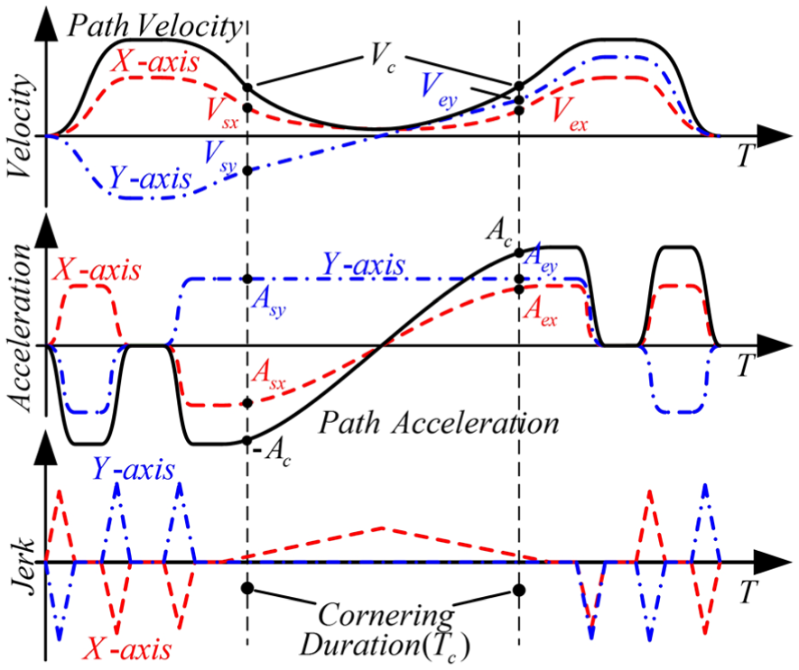
Velocity, acceleration, and jerk profiles.

The velocity transition for X-axis can be obtained from equation (2)

$$\mathrm{\Delta }{V}_x=V_C|\cos ({\theta }_e)-\cos ({\theta }_s)|$$

(3)

where θ _s and θ _e are the angles at the beginning and end of the corner motion, respectively. θ _ε is the error angle. The maximum contour error is ε, which is set by the program. The contour error of X-axis at the maximum contour error is

$${\epsilon }_x=\epsilon \cos \left({\theta }_{\epsilon }\right)=x_{\mathrm{mid}}-x_C$$

(4)

where θ _ε =π/2 + (θ _s  + θ _e )/2 can be derived from the corner profile of Figure 1. The Y-axis equations need to replace the sine term with the cosine term. R_c is the linear displacement during cornering motion, which can be deduced from equation (1)

$$\begin{array}{l}{R}_C=\left|\frac{\left[\begin{array}{ccc}{V}_{sx}& A_{sx}& S_x\end{array}\right]{\left[\begin{array}{ccc}2T_1& 2T_1^2& \frac{7}{12}{T}_1^4\end{array}\right]}^{\prime }}{\cos ({\theta }_s)+\cos ({\theta }_e)}\right|\\ =\left|\frac{\left[\begin{array}{ccc}{V}_{sy}& A_{sy}& S_y\end{array}\right]{\left[\begin{array}{ccc}2T_1& 2T_1^2& \frac{7}{12}{T}_1^4\end{array}\right]}^{\prime }}{\sin ({\theta }_s)+\sin ({\theta }_e)}\right|\end{array}$$

(5)

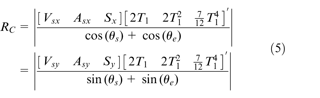
To achieve the optimal feed strategy, the minimum cornering duration T_c can be achieved by setting the limit axis jounce or acceleration at least 1 to reach the saturation of the drive. The limit axis can be determined by equation (3). If ΔV_x > ΔV_y, then the X-axis is the limit axis and the minimum cornering duration can be calculated by the X-axis velocity, acceleration, and maximum contour error constraints

$$\{\begin{array}{l}{A}_C\cos ({\theta }_e)=-A_C\cos ({\theta }_s)+S_x{T}_1^2\\ V_C\cos ({\theta }_e)=V_C\cos ({\theta }_s)-2A_C\cos ({\theta }_s)T_1+S_x{T}_1^3\\ \epsilon \cos ({\theta }_{\epsilon })=\frac{V_C\cos ({\theta }_s)T_1\left(\cos ({\theta }_e)-\cos ({\theta }_s)\right)-A_C\cos \left({\theta }_s\right)T_1^2\left(\frac{1}{2}\cos ({\theta }_e)-\frac{3}{2}\cos ({\theta }_s)\right)+S_x{T}_1^4\left(\frac{1}{24}\cos ({\theta }_e)-\frac{13}{24}\cos ({\theta }_s)\right)}{\cos ({\theta }_s)+\cos ({\theta }_e)}\end{array}$$

(6)

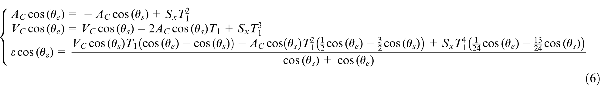
The three constraint equations have four unknowns, S_x, A_c, V_c, T₁, which can be calculated by setting the limit axis jounce or acceleration saturation.

When the limit axis jounce is saturated, S_x = S_max

$$\{\begin{array}{c}{A}_C=\sqrt{\left|\frac{24\epsilon \cos ({\theta }_{\epsilon })S_x}{({\cos }^2({\theta }_e)-{\cos }^2({\theta }_s))}\right|}\hfill \\ \multicolumn{1}{c}{V_C=\sqrt[4]{\left|\frac{{24}^3{\epsilon }^3{\cos }^3({\theta }_{\epsilon })S_x}{(\cos ({\theta }_e)+\cos ({\theta }_s)){(\cos ({\theta }_e)-\cos ({\theta }_s))}^3}\right|}}\\ \multicolumn{1}{c}{T_1=\sqrt[4]{\left|\frac{24\epsilon \cos ({\theta }_{\epsilon })(\cos ({\theta }_s)+\cos ({\theta }_e))}{(\cos ({\theta }_e)-\cos ({\theta }_s))S_x}\right|}}\\ \multicolumn{1}{c}{R_C=\frac{14\epsilon \cos ({\theta }_{\epsilon })}{(\cos ({\theta }_e)-\cos ({\theta }_s))}}\end{array}$$

(7)

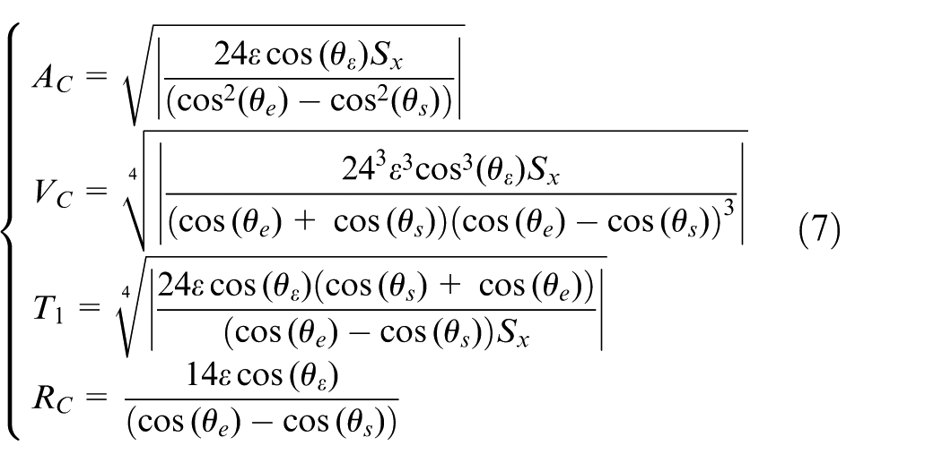
When the limit axis acceleration is saturated, A_c = A_max

$$\{\begin{array}{c}{S}_x=\frac{{A_C}^2({\cos }^2({\theta }_e)-{\cos }^2({\theta }_s))}{24\epsilon \cos ({\theta }_{\epsilon })}\hfill \\ \multicolumn{1}{c}{V_C=\sqrt{\frac{24A_C\epsilon \cos ({\theta }_{\epsilon })}{(\cos ({\theta }_e)-\cos ({\theta }_s))}}}\\ \multicolumn{1}{c}{T_1=\sqrt{\frac{24\epsilon \cos ({\theta }_{\epsilon })}{A_C(\cos ({\theta }_e)-\cos ({\theta }_s))}}}\\ \multicolumn{1}{c}{R_C=\frac{14\epsilon \cos ({\theta }_{\epsilon })}{(\cos ({\theta }_e)-\cos ({\theta }_s))}}\end{array}$$

(8)

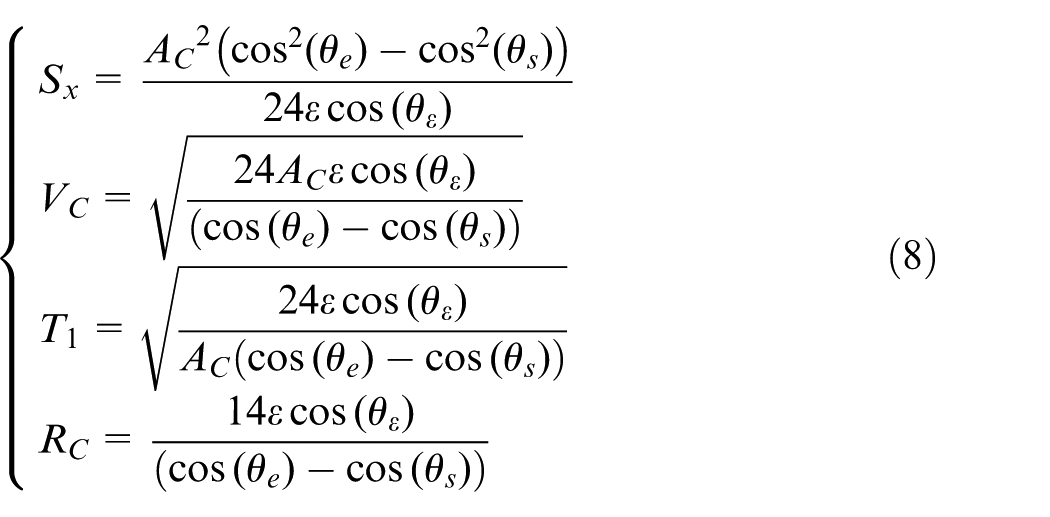
In order to control the drive system within the motion limit, V_c value is

$$V_C=min\{V_{\mathrm{CSmax}},V_{\mathrm{CAmax}}\}$$

(9)

In the X–Y plane motion, the X-axis is calculated as the limit axis by equation (6) to achieve the continuous feed motion strategy, and the limit axis saturates either jounce or acceleration limits of the drives to achieve the balance of time optimization and drive performance. When the Y-axis is the limit axis, the corresponding parameters can be obtained by replacing the sine with the cosine. It is noteworthy that when the corner is particularly blunt, the calculated cornering transition velocity V_c may exceed the value F set by the numerical control (NC) program. In this case, the cornering transition velocity is set as F, and the corresponding parameters are calculated by F.

Uninterrupted global motions with smoothed acceleration

Figure 3 shows the machining path planned by the NC program. The corner of each path can be used to realize the uninterrupted feed motion of the corners through the corner smoothing technique introduced in section “Uninterrupted cornering motions with smoothed acceleration.” From equations (7) and (8), the maximum cornering transition velocity V_c and acceleration A_c for each corner can be determined and a series of corner boundary conditions can be read to plan the uninterrupted feed motion between corners as shown in Figure 4 for the feed strategy base on look-ahead interpolation algorithm. At the beginning of the interpolation motion, the velocity of the feed motion at the end of the path $P_C^N$ is zero and the feed motion is planned in the previous path. During the planning, the current feed velocity is reduced to ensure that the motion can be interpolated, and once the current motion accepts the planned interpolation motion, only the compatibility of the kth corner and the k + 1th corner is considered. This interpolation method does not require any iteration, and it can achieve rapid interpolation planning. The following section details the calculation of the algorithm parameters.

Figure 3.

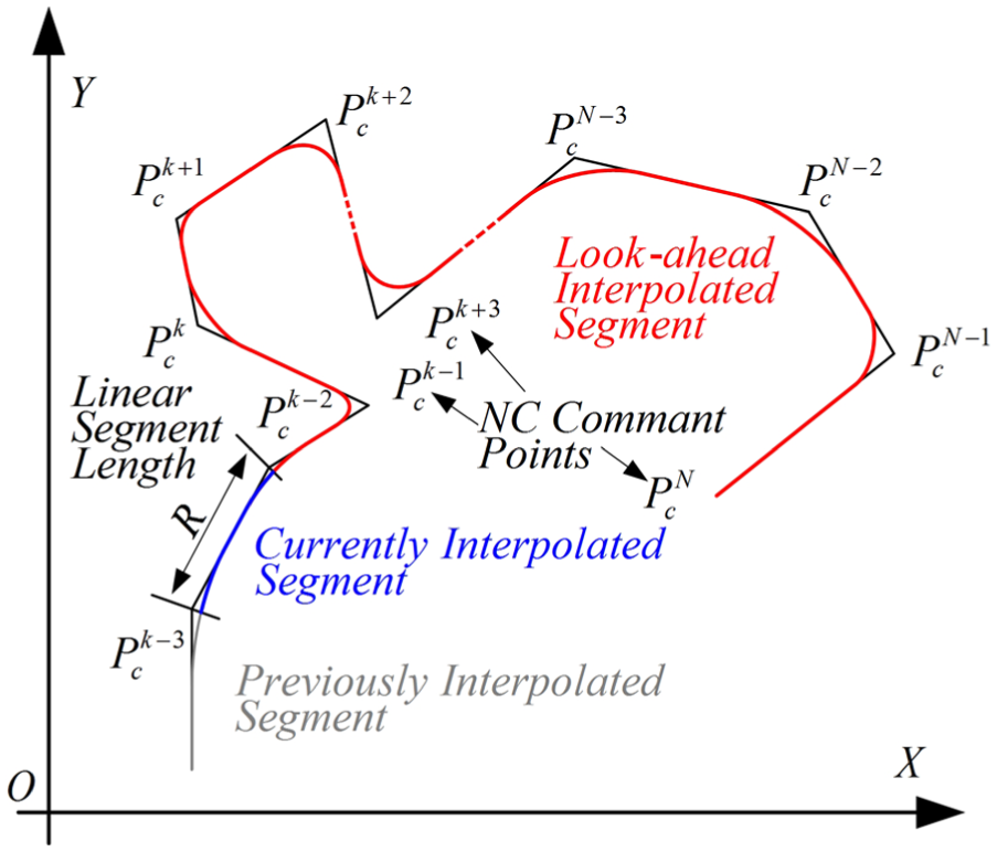
Global motion planning strategy.

Figure 4.

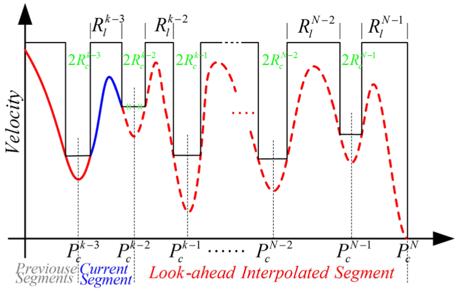
Feedrate planning in global motion.

Motion planning along separated corners

Through the uninterrupted feed motion of the corner introduced in the first section, the transition distance $R_c^k$ for each corner can be precisely calculated from equation (5). Then, the remaining linear segment distance

$$R_l^k=\Vert P_c^k-P_c^{k+1}\Vert -(R_c^k+R_c^{k+1})$$

(10)

If $R_l^k>0$ , then the kth corner and the k + 1th corner will not overlap; each corner is the independent corner, as shown in Figure 5. The smooth transition of velocity and acceleration between the two corners is achieved by planning the kinematic boundary conditions at the two corners of the front and back, as shown in Figure 6. The algorithm utilizes the 11-segmented jounce-limited acceleration curve to stitch the feed contour at both corners to achieve maximum feed velocity while smoothing the acceleration and velocity transitions, as shown in Figure 7. The maximum feed velocity V_m is obtained by adding the boundary condition speeds $V_c^k$ , $V_{c+1}^k$ and accelerations $A_c^k$ , $A_c^{k+1}$

$$v(\tau )=\{\begin{array}{l}{V}_c^k+A_c^k{\tau }_1+\frac{1}{6}{S}_m{\tau }_1^3,0\le t<t_1,V_1=V_c^k+A_c^k{T}_1+\frac{1}{6}{S}_m{T}_1^3\\ V_1+A_1{\tau }_2-\frac{1}{6}{S}_m{\tau }_2^3+\frac{1}{2}{S}_m{T}_1{\tau }_2^2,t_1\le t<t_2,V_2=V_1+A_1{T}_2-\frac{1}{6}{S}_m{T}_2^3+\frac{1}{2}{S}_m{T}_1{T}_2^2\\ V_2+A_p{\tau }_3,t_2\le t<t_3,V_3=V_2+A_p{T}_3\\ V_3+A_p{\tau }_4-\frac{1}{6}{S}_m{\tau }_4^3,t_3\le t<t_4,V_4=V_3+A_p{T}_4-\frac{1}{6}{S}_m{T}_4^3\\ V_4+A_4{\tau }_5+\frac{1}{6}{S}_m{\tau }_5^3-\frac{1}{2}{S}_m{T}_4{\tau }_5^2,t_4\le t<t_5,V_5=V_4+A_4{T}_5+\frac{1}{6}{S}_m{T}_5^3-\frac{1}{2}{S}_m{T}_4{T}_5^2\\ V_m,t_5\le t<t_6,V_m=V_5\\ V_m-\frac{1}{6}{S}_m{\tau }_7^3,t_6\le t<t_7,V_7=V_m-\frac{1}{6}{S}_m{T}_7^3\\ V_7+A_7{\tau }_8+\frac{1}{6}{S}_m{\tau }_8^3-\frac{1}{2}{S}_m{T}_7{\tau }_8^2,t_7\le t<t_8,V_8=V_7+A_7{T}_8+\frac{1}{6}{S}_m{T}_8^3-\frac{1}{2}{S}_m{T}_7{T}_8^2\\ V_8+A_n{\tau }_9,t_8\le t<t_9,V_9=V_8+A_n{T}_9\\ V_9+A_n{\tau }_{10}+\frac{1}{6}{S}_m{\tau }_{10}^3,t_9\le t<t_{10},V_{10}=V_9+A_n{T}_{10}+\frac{1}{6}{S}_m{T}_{10}^3\\ V_{10}+A_{10}{\tau }_{11}-\frac{1}{6}{S}_m{\tau }_{11}^3+\frac{1}{2}{S}_m{T}_{10}{\tau }_{11}^2,t_{10}\le t<t_{11},V_c^{k+1}=V_{10}+A_{10}{T}_{11}-\frac{1}{6}{S}_m{T}_{11}^3+\frac{1}{2}{S}_m{T}_{10}{T}_{11}^2\end{array}$$

(11)

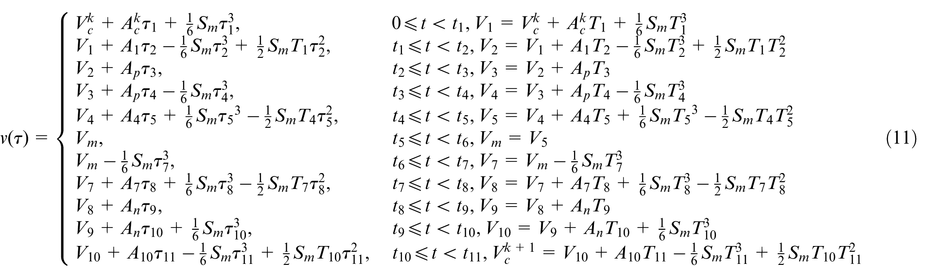
where t_i is the relative time boundary of each phase, which is calculated from the beginning of each phase. T_i is the duration of each phase. V_m is the maximum feed velocity in the linear segments and V_i is the velocity reached at the end of each phase. The displacement curve can be obtained by integrating the velocity curve.

Figure 5.

Motion planning along separated corners.

Figure 6.

Jounce-limited acceleration profile.

Figure 7.

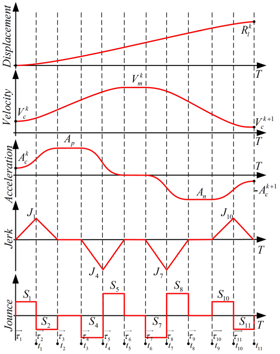
Motion planning along overlapping corners.

The duration of each phase is calculated by equation (11)

$$\begin{array}{c}{T}_1=T_2=\sqrt{\frac{A_p-A_c^k}{S_m}},T_4=T_5=\sqrt{\frac{A_p}{S_m}},\hfill \\ T_3=\frac{V_m-V_c^k}{A_p}-2\sqrt{\frac{A_p}{S_m}}+\sqrt{\frac{{A_c^k}^3}{{A_p}^2{S}_m}}\hfill \\ T_7=T_8=\sqrt{\frac{A_n}{-S_m}},T_{10}=T_{11}=\sqrt{\frac{A_c^{k+1}-A_n}{S_m}},\hfill \\ T_9=\frac{V_c^{k+1}-V_m}{A_n}-2\sqrt{\frac{A_n}{-S_m}}+\sqrt{\frac{A_c^{k+13}}{-{A_n}^2{S}_m}}\hfill \end{array}$$

(12)

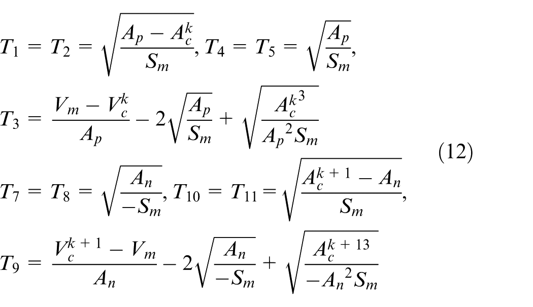
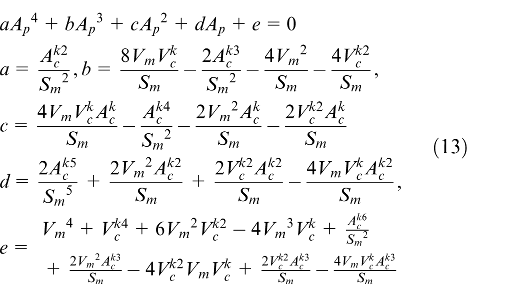
When the duration time T₃ and T₉ calculated by equation (12) are less than zero, the constant acceleration phase does not exist. Set T₃ = T₉ = 0 and the maximum acceleration is recalculated by the following quartic equation

$$\begin{array}{c}a{A_p}^4+b{A_p}^3+c{A_p}^2+d{A}_p+e=0\hfill \\ a=\frac{A_c^{k2}}{{S_m}^2},b=\frac{8V_m{V}_c^k}{S_m}-\frac{2A_c^{k3}}{{S_m}^2}-\frac{4{V_m}^2}{S_m}-\frac{4V_c^{k2}}{S_m},\hfill \\ c=\frac{4V_m{V}_c^k{A}_c^k}{S_m}-\frac{A_c^{k4}}{{S_m}^2}-\frac{2{V_m}^2{A}_c^k}{S_m}-\frac{2V_c^{k2}{A}_c^k}{S_m}\hfill \\ d=\frac{2A_c^{k5}}{{S_m}^5}+\frac{2{V_m}^2{A}_c^{k2}}{S_m}+\frac{2V_c^{k2}{A}_c^{k2}}{S_m}-\frac{4V_m{V}_c^k{A}_c^{k2}}{S_m},\hfill \\ e=\begin{array}{c}\begin{array}{c}{V_m}^4+V_c^{k4}+6{V_m}^2{V}_c^{k2}-4{V_m}^3{V}_c^k+\frac{A_c^{k6}}{{S_m}^2}\hfill \\ \multicolumn{1}{c}{+\frac{2{V_m}^2{A}_c^{k3}}{S_m}-4V_c^{k2}{V}_m{V}_c^k+\frac{2V_c^{k2}{A}_c^{k3}}{S_m}-\frac{4V_m{V}_c^k{A}_c^{k3}}{S_m}}\end{array}\hfill \end{array}\hfill \end{array}$$

(13)

The distance between the corners $L_l^k$ should be obtained by the interpolation displacement for all phases. If $L_l^k$ is long enough, the maximum feed velocity V_m reaches the maximum velocity set by the NC program, and if there is a uniform phase T₆ > 0, then the total displacement of the 11-segmented jounce-limited acceleration curve is as follows

$$\begin{array}{c}{L}_l^k=V_m{T}_6+\frac{2(V_c^k\sqrt{A_p-A_c^k}+V_c^{k+1}\sqrt{A_c^{k+1}-A_n})}{\sqrt{S_m}}\hfill \\ +\frac{5(A_c^k{A}_p+A_c^{k+1}{A}_n)}{6S_m}-\frac{17(A_c^{k2}+A_c^{k+12})}{12S_m}\hfill \\ +\frac{V_m^2}{2}(\frac{1}{A_p}-\frac{1}{A_n})+\frac{V_m(\sqrt{A_p}+\sqrt{-A_n})}{\sqrt{S_m}}\hfill \\ -\frac{(V_c^k\sqrt{A_p}+V_c^{k+1}\sqrt{-A_n})}{\sqrt{S_m}}\hfill \\ +\frac{(A_c^k\sqrt{A_p{A}_c^k}-A_c^{k+1}\sqrt{A_n{A}_c^{k+1}})}{S_m}\hfill \\ +\frac{1}{2}(\frac{V_c^{k+12}}{A_n}-\frac{V_c^{k2}}{A_p})-\frac{1}{2S_m}(\frac{A_c^{k+13}}{A_n}+\frac{A_c^{k3}}{A_p})\hfill \\ +\frac{1}{\sqrt{S_m}}(\frac{V_c^{k+1}\sqrt{-{(A_c^{k+1})}^3}}{A_n}+\frac{V_c^k\sqrt{{(A_c^k)}^3}}{A_p})\hfill \end{array}$$

(14)

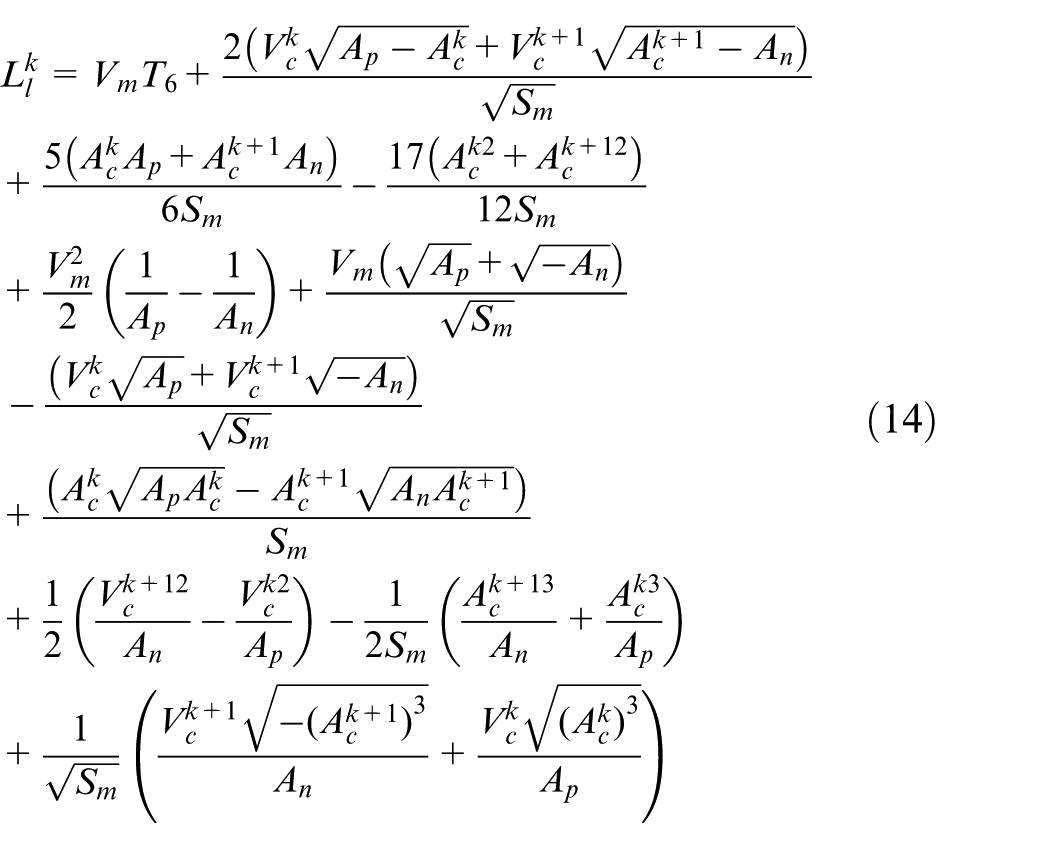
If T₆ < 0 is calculated by equation (14), then the constant velocity phase does not exist. The feed velocity does not reach the commanded maximum velocity, and V_m is recalculated as follows

$$\begin{array}{c}a{V_m}_{\mathrm{new}}^2+b{V_m}_{\mathrm{new}}+c=0,\hfill \\ \mathrm{where}:a=\frac{1}{2A_p}-\frac{1}{2A_n},b=\frac{V_m(\sqrt{A_p}+\sqrt{-A_n})}{\sqrt{S_m}}\hfill \\ c=\frac{2(V_c^k\sqrt{A_p-A_c^k}+V_c^{k+1}\sqrt{A_c^{k+1}-A_n})}{\sqrt{S_m}}\hfill \\ +\frac{5(A_c^k{A}_p+A_c^{k+1}{A}_n)}{6S_m}-\frac{17(A_c^{k2}+A_c^{k+12})}{12S_m}\hfill \\ -\frac{(V_c^k\sqrt{A_p}+V_c^{k+1}\sqrt{-A_n})}{\sqrt{S_m}}+\frac{(A_c^k\sqrt{A_p{A}_c^k}-A_c^{k+1}\sqrt{A_n{A}_c^{k+1}})}{S_m}\hfill \\ +\frac{1}{2}(\frac{V_c^{k+12}}{A_n}-\frac{V_c^{k2}}{A_p})-\frac{1}{2S_m}(\frac{A_c^{k+13}}{A_n}+\frac{A_c^{k3}}{A_p})\hfill \\ +\frac{1}{\sqrt{S_m}}(\frac{V_c^{k+1}\sqrt{-\left(A_c^{k+13}\right)}}{A_n}+\frac{V_c^k\sqrt{{\left(A_c^k\right)}^3}}{A_p})\hfill \end{array}$$

(15)

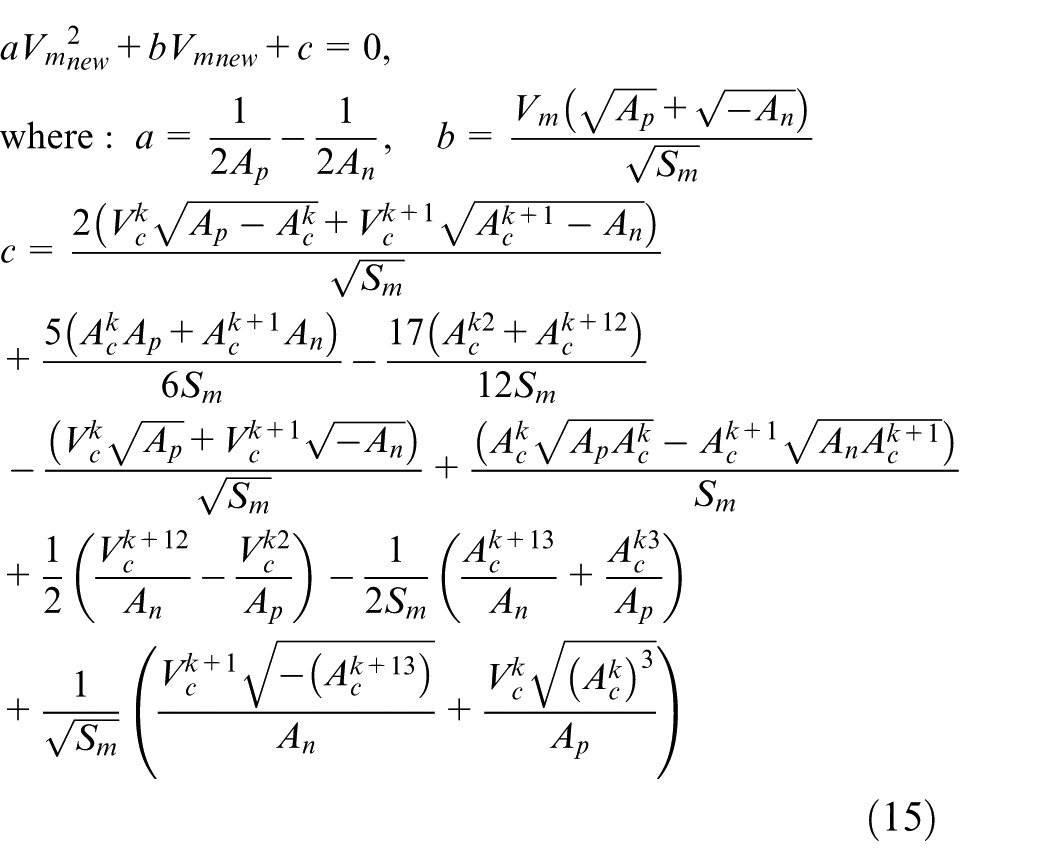
If V_m calculated by equation (15) has complex roots, the maximum cornering velocity $V_c^k$ and $V_c^{k+1}$ need to be adjusted to find the optimal velocity. The traditional iterative algorithm can be used to find the optimal cornering velocity, but the iterative algorithm requires deep loop to find the appropriate $V_c^k$ and $V_c^{k+1}$ , so this method is not suitable for real-time high-speed motion. As a result, it is necessary to study a more accurate and direct method for finding optimal $V_c^k$ and $V_c^{k+1}$ .

The cornering velocity is reduced to the minimum

$$V_c^k=V_c^{k+1}=min\{V_c^k,V_c^{k+1}\}$$

(16)

While reducing the cornering velocity, the maximum contour error is also reduced. Meanwhile, the length $R_c^k$ of the linear segment required at the corner is reduced and $R_l^k$ is extended, and the uninterrupted feed motion can be achieved by equation (14). Based on the minimum cornering velocity, the transition algorithm between separated corners is further studied to search for the feasible cornering velocity.

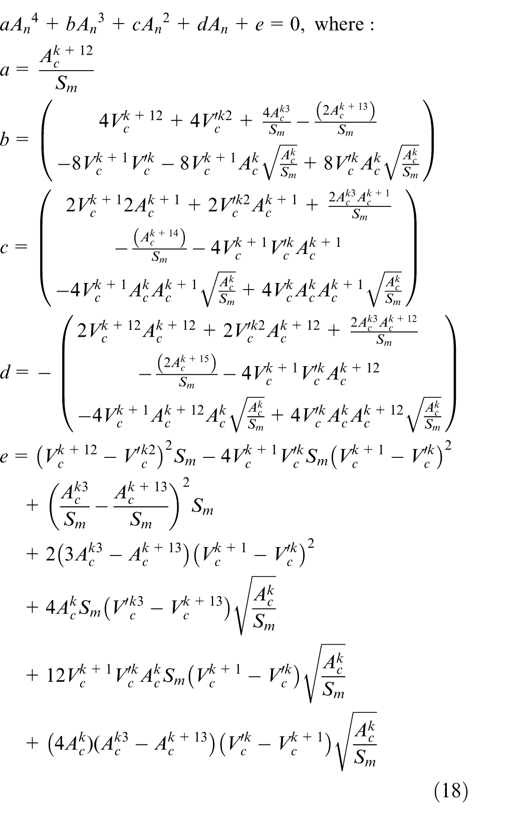
First, if the linear segment between corners is very short, it is not realistic to plan a complete 11-segmented jounce-limited acceleration curve and replace the original 11-segmented with 6-segmented jounce-limited acceleration curve. Then, assuming constant velocity does not exist in original 11-segmented jounce-limited acceleration curve and the duration of the constant velocity phase is zero, T₃ = T₆ = T₉ = 0, and it is assumed that if $V_c^k>V_c^{k+1}$ , the acceleration phase does not exist, T₁ = T₂ = 0. Similarly, if $V_c^{k+1}>V_c^k$ , the deceleration increase phase does not exist, that is, T₁₀ = T₁₁ = 0. Finally, the original 11-segmented jounce-limited acceleration curve was shortened to 6-segmented curve. The optimal $V_c^k$ and $A_c^k$ are calculated with 6-segmented jounce-limited acceleration curve to achieve the smooth transition of the short linear segments between separated corner profiles. The following relationships are established by contour error, optimal transition velocity, acceleration, and the length of the corner profiles. The duration of each phase is

$$\begin{array}{l}\begin{array}{l}{A^{\prime }}_c^k=\sqrt{\alpha }{A}_c^k\\ {V^{\prime }}_c^k=\alpha V_c^k\\ {R^{\prime }}_c^k={\alpha }^2{R}_c^k\end{array}\},T_4=T_5=\sqrt{\frac{{A^{\prime }}_c^k}{S_m}},\\ T_7=T_8=\sqrt{\frac{A_n}{-S_m}},T_{10}=T_{11}=\sqrt{\frac{A_c^{k+1}-A_n}{S_m}}\end{array}$$

(17)

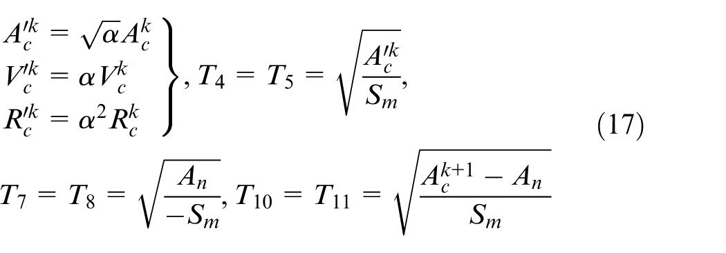
The maximum acceleration A_n can be calculated by the following equation

$$\begin{array}{c}a{A_n}^4+b{A_n}^3+c{A_n}^2+d{A}_n+e=0,\mathrm{where}:\hfill \\ a=\frac{A_c^{k+12}}{S_m}\hfill \\ b=\left(\begin{array}{c}4V_c^{k+12}+4V{\prime }_c^{k2}+\frac{4A_c^{k3}}{S_m}-\frac{\left(2A_c^{k+13}\right)}{S_m}\hfill \\ \multicolumn{1}{c}{-8V_c^{k+1}V{\prime }_c^k-8V_c^{k+1}{A}_c^k\sqrt{\frac{A_c^k}{S_m}}+8V{\prime }_c^k{A}_c^k\sqrt{\frac{A_c^k}{S_m}}}\end{array}\right)\hfill \\ c=\left(\begin{array}{c}2V_c^2{A}_c^{k+1}+2V{\prime }_c^{k2}{A}_c^{k+1}+\frac{2A_c^{k3}{A}_c^{k+1}}{S_m}\hfill \\ \multicolumn{1}{c}{-\frac{\left(A_c^{k+14}\right)}{S_m}-4V_c^{k+1}V{\prime }_c^k{A}_c^{k+1}}\\ \multicolumn{1}{c}{-4V_c^{k+1}{A}_c^k{A}_c^{k+1}\sqrt{\frac{A_c^k}{S_m}}+4V_c^k{A}_c^k{A}_c^{k+1}\sqrt{\frac{A_c^k}{S_m}}}\end{array}\right)\hfill \\ d=-\left(\begin{array}{c}2V_c^{k+12}{A}_c^{k+12}+2V{\prime }_c^{k2}{A}_c^{k+12}+\frac{2A_c^{k3}{A}_c^{k+12}}{S_m}\hfill \\ \multicolumn{1}{c}{-\frac{\left(2A_c^{k+15}\right)}{S_m}-4V_c^{k+1}V{\prime }_c^k{A}_c^{k+12}}\\ \multicolumn{1}{c}{-4V_c^{k+1}{A}_c^{k+12}{A}_c^k\sqrt{\frac{A_c^k}{S_m}}+4V{\prime }_c^k{A}_c^k{A}_c^{k+12}\sqrt{\frac{A_c^k}{S_m}}}\end{array}\right)\hfill \\ e={(V_c^{k+12}-{V\prime }_c^{k2})}^2{S}_m-4V_c^{k+1}V{\prime }_c^k{S}_m{(V_c^{k+1}-V{\prime }_c^k)}^2\hfill \\ +{(\frac{A_c^{k3}}{S_m}-\frac{A_c^{k+13}}{S_m})}^2{S}_m\hfill \\ +2(3A_c^{k3}-A_c^{k+13}){(V_c^{k+1}-V{\prime }_c^k)}^2\hfill \\ +4A_c^k{S}_m({V\prime }_c^{k3}-V_c^{k+13})\sqrt{\frac{A_c^k}{S_m}}\hfill \\ +12V_c^{k+1}V{\prime }_c^k{A}_c^k{S}_m(V_c^{k+1}-V{\prime }_c^k)\sqrt{\frac{A_c^k}{S_m}}\hfill \\ +(4A_c^k)(A_c^{k3}-A_c^{k+13})(V{\prime }_c^k-V_c^{k+1})\sqrt{\frac{A_c^k}{S_m}}\hfill \end{array}$$

(18)

The maximum deceleration A_p can be achieved by swapping $V_c^k$ and $V_c^{k+1}$ , $A_c^k$ and $A_c^{k+1}$ . The function for α can be obtained

$$\begin{array}{l}{\alpha }^2{L}_c^k+2V_c^k\left(\sqrt{\frac{-A_n}{S_m}}+\sqrt{\frac{A_c^k}{S_m}}\right)\alpha +\frac{17}{12}\frac{{A_c^k}^2}{S_m}\\ -\frac{13}{6}\frac{{A_c^{k+1}}^2}{S_m}+\frac{19}{12}\frac{A_c^{k+1}{A}_n}{S_m}+2A_c^k\sqrt{\frac{-A_n{A}_c^k}{S_m^2}}\\ +2V_c^{k+1}\sqrt{\frac{\left(A_c^{k+1}-A_n\right)}{S_m}}-L_c^k-L_l^k=0\end{array}$$

(19)

A_n and α can be achieved by equations (18) and (19) so that the optimal transition velocity can be obtained by equation (15). This method calculates a feasible solution of the optimal transition velocity by the parameter α, avoids deep iterative problems and greatly reduces the time consumed by the calculation.

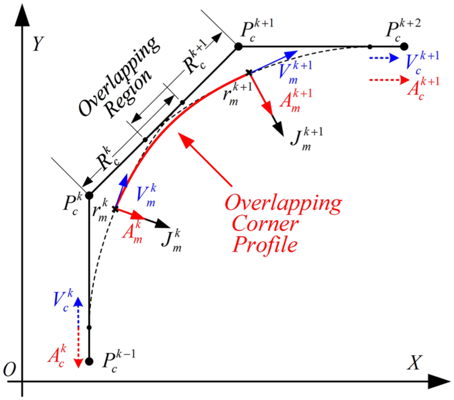
Motion planning along overlapping corners

This section presents the interpolation algorithm for smoothing linear segments with overlapping corner contours, as shown in Figure 8. For overlapping corner contours, the plan is to transition the midpoint of the two corner contours to generate a high-speed transition trajectory, as shown in Figure 9. The velocity, acceleration and jerk values at the midpoint of the two corner profiles are stitched by the 4-segmented jounce-limited acceleration curve to achieve the smooth transition of acceleration, as shown in Figure 10.

Figure 8.

Speed and acceleration stitching at the separated corner.

Figure 9.

Contour stitching at overlapping corners.

Figure 10.

Speed and acceleration stitching at overlapping corners.

The midpoint of each corner of the parameter values can be written as

$$\begin{array}{l}{j}_{mx}^k=S_x^k{T}_1^k\\ a_{mx}^k=A_{sx}^k+\frac{1}{2}{S}_x^k{T_1^k}^2\\ v_{mx}^k=V_{sx}^k+A_{sx}^k{T}_1^k+\frac{1}{6}{S}_x^k{T_1^k}^3\\ r_{mx}^k={\epsilon }_x^k+x_c^k\end{array}\}\mathrm{and}\{\begin{array}{l}{j}_{my}^k=S_y^k{T}_1^k\\ a_{my}^k=A_{sy}^k+\frac{1}{2}{S}_y^k{T_1^k}^2\\ v_{my}^k=V_{sy}^k+A_{sy}^k{T}_1^k+\frac{1}{6}{S}_y^k{T_1^k}^3\\ r_{my}^k={\epsilon }_y^k+x_c^k\end{array}$$

(20)

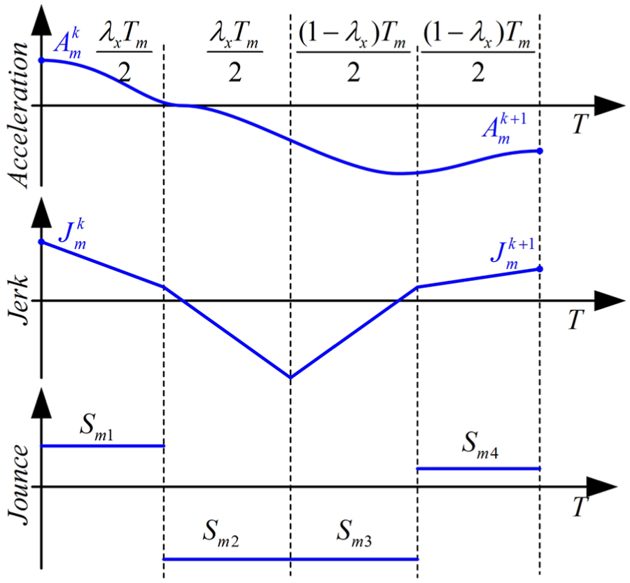
T ₁ represents the duration of the first phase of the corner smoothing algorithm introduced in section “Uninterrupted cornering motions with smoothed acceleration.” Take the X-axis as an example, the boundary conditions of jerk, acceleration, velocity, and displacement can be written as

$$\begin{array}{c}{j}_{\mathrm{mx}}^{k+1}=j_{\mathrm{mx}}^k-(S_{m1x}+S_{m2x})\frac{\lambda T_m}{2}+(S_{m3x}+S_{m4x})\frac{(1-\lambda )T_m}{2}\hfill \\ A_{\mathrm{mx}}^{k+1}=A_{\mathrm{mx}}^k+j_{\mathrm{mx}}^k{T}_m-\lambda (1-\lambda )(S_{m1x}+S_{m2x})\frac{T_m^2}{2}\hfill \\ +(3S_{m3x}+S_{m4x})\frac{{(1-\lambda )}^2{T}_m^2}{8}-(3S_{m1x}+S_{m2x})\frac{{\lambda }^2{T}_m^2}{8}\hfill \\ V_{\mathrm{mx}}^{k+1}=V_{\mathrm{mx}}^k+2A_{\mathrm{mx}}^k\left(\frac{T_m}{2}\right)+2j_{\mathrm{mx}}^k\frac{T_m^2}{4}\hfill \\ -(7S_{m1x}+S_{m2x}){\lambda }^3\frac{T_m^3}{48}+(7S_{m3x}+S_{m4x})(1-\lambda {)}^3\frac{T_m^3}{48}\hfill \\ -(\lambda (3S_{m1x}+S_{m2x})+(1-\lambda )(2S_{m1x}+2S_{m2x}))\lambda (1-\lambda )\frac{T_m^3}{8}\hfill \\ R_{\mathrm{mx}}^{k+1}=R_{\mathrm{mx}}^k+V_{\mathrm{mx}}^k{T}_m+\frac{A_{\mathrm{mx}}^k{T_m}^2}{2}+\frac{j_{\mathrm{mx}}^k{T_m}^3}{6}\hfill \\ -(15S_{m1x}+S_{m2x})\frac{{\lambda }^4{T}_m^4}{384}+(15S_{m3x}+S_{m4x})(1-\lambda {)}^4\frac{T_m^4}{384}\hfill \\ -(7S_{m1x}+S_{m2x}){\lambda }^3(1-\lambda )\frac{T_m^4}{48}-(3S_{m1x}+S_{m2x})\hfill \\ {\lambda }^2(1-\lambda {)}^2\frac{T_m^4}{16}-(S_{m1x}+S_{m2x})(1-\lambda {)}^3\lambda \frac{T_m^4}{12}\hfill \end{array}$$

(21)

where T_m is the total duration of the motion, S_m1–S_m4 is the jounce values of each phase, and there are 11 unknowns in the X-axis and Y-axis, S_m1x–S_m4x, S_m1y–S_m4y, λ_x, λ_y and T_m. However, based on only eight equations, it is essential to increase the boundary conditions. When λ_x = 0.5 and S_m2x = –S_m3x, T_m can be determined by four constraints on the X-axis, as shown in equation (22). The same method can be used with T_m to find the unknown of the Y-axis

$$\{\begin{array}{l}\frac{4j_{mx}^{k+1}-4j_{mx}^k}{T_m}=S_{m4x}\\ \left(57S_{m1x}+23S_{m2x}\right)=\left(2R_{mx}^{k+1}-2R_{mx}^k+\left(7j_{mx}^{k+1}+121j_{mx}^k\right)\frac{T_m^3}{768}-V_{mx}^k{T}_m-V_{mx}^{k+1}{T}_m\right)\frac{1536}{T_m^4}\\ \left(3S_{m1x}+S_{m2x}\right)=\frac{\left(2j_{mx}^{k+1}+14j_{mx}^k\right)}{T_m}\\ \left(\frac{5j_{mx}^k}{96}-\frac{5j_{mx}^{k+1}}{96}\right)T_m^2+\left(\frac{A_{mx}^{k+1}}{2}+\frac{A_{mx}^k}{2}\right)T_m+V_{mx}^k-V_{mx}^{k+1}=0\end{array}$$

(22)

According to the above equation, uninterrupted feed motion between overlapping corners can be realized, and the contour trajectory of two corners can be mixed to achieve the smooth transition of acceleration. With this, uninterrupted feed motion planning is performed for the corners, the separated corner contours and the overlapping corner contours, to achieve uninterrupted feed motion of the global tool-path. At the same time, the G² continuous acceleration curve is realized based on jounce-limited acceleration curve.

Simulation and experimental results

Simulation results

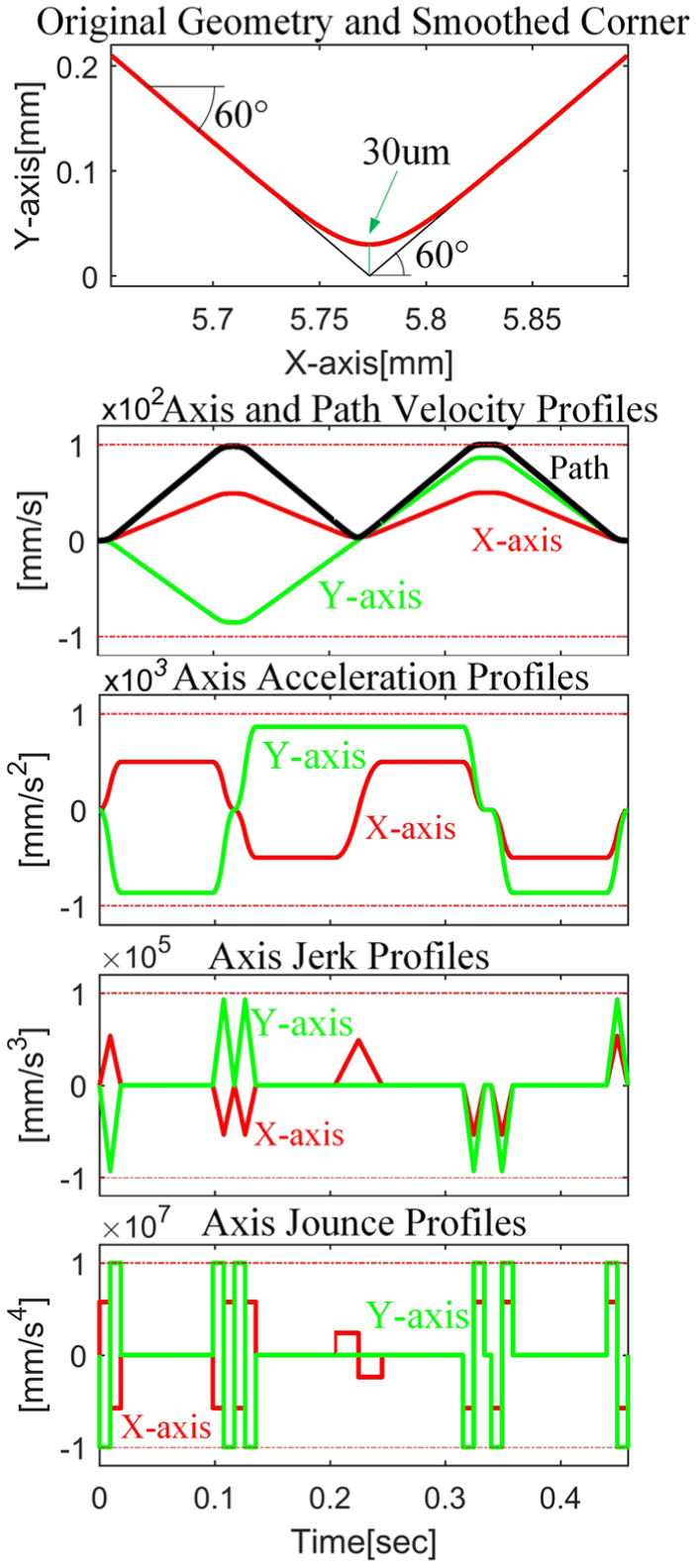
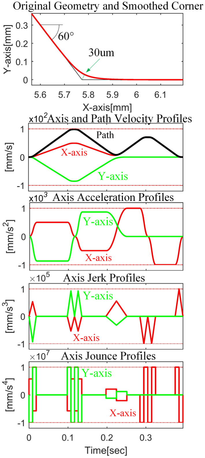
This section includes simulation and experiments of the global uninterrupted feed motion technology described in the previous section. First, the cornering interpolation algorithm is simulated. Figure 11 shows a 60° acute feed motion and Figure 12 shows a 120° obtuse feed motion. The path lengths for acute and obtuse angles are both 23.08 mm and the contour error is set to 30 μm in both cases. The maximum feed speed of the drive is 100 mm/s, the acceleration limit is 1000 mm/s², and the jounce limit is 1 × 10⁷ mm/s⁴. The maximum cornering velocity of the acute angle is 20.39 mm/s². The machining time is 0.456 s, and the duration of the corner transition is 0.041 s. The maximum cornering velocity of the obtuse angle is 26.84 mm/s². The machining time is 0.395 s, and the duration of the corner transition is 0.054 s.

Figure 11.

Acute angle motion feed strategy.

Figure 12.

Obtuse angle motion feed strategy.

The maximum cornering velocity for the acute angle is relatively smaller, and the duration of cornering transition motion is shorter in that the length of the corner transition profile is relatively shorter, leading to longer remaining linear segments and total machining time. The reason for obtuse angle machining parameters is the opposite. The simulation results demonstrate that the cornering interpolation algorithm generates the corner contour trajectory around the corner. The contour trajectory can precisely control the contour error, and the generated acceleration curve reaches G² continuous. At the same time, the acceleration or the jounce of at least one axis reaches the maximum limit of the drive for the fastest cornering transition motion.

Then, the interpolation algorithm of short linear segments between corner contours is simulated. The motion planning along separated corners (MPASC) described in section “Motion planning along separated corners” and the motion planning along overlapping corners (MPAOC) described in section “Motion planning along overlapping corners” are shown in Figures 13 and 14, respectively. The total length of the machining path is 17 mm, the length of the linear segment between two corner points is 1 mm, and two obtuse angles are 143.13° and 126.98° respectively. Set the maximum feed velocity and the maximum acceleration the same as the previous, and the jounce limit is 2 × 10⁷ mm/s⁴. The maximum contour error of the separated corner feed strategy is set to 10 µm, and the maximum contour error of the overlapping corner feed strategy is set to 100 µm. The total machining time for the separated corners feed strategy is 0.4442 s, and the duration of the feed motion for the short linear segment is 0.028 s. The total machining time of the overlapping corner feed strategy is 0.418 s, and the duration of the feed motion for the mixed two corner contours is 0.054 s. When the contour error increases, the total machining time is reduced. The machining time with the contour error of 100 μm is reduced by nearly 6% compared to the machining time of 10 μm. The maximum feed velocity of the MPASC algorithm is 25.81 mm/s and the minimum feed velocity is 4.88 mm/s, and the maximum feed velocity of the MPAOC algorithm is 23.21 mm/s and the minimum feed velocity is 15.46 mm/s. It is found from the simulation that when the corner contour error increases, the feed velocity between the corners tends to be high and steady. Take full advantage of the driver’s motion performance and keep the acceleration curve G² continuous, which brings smooth acceleration transition.

Figure 13.

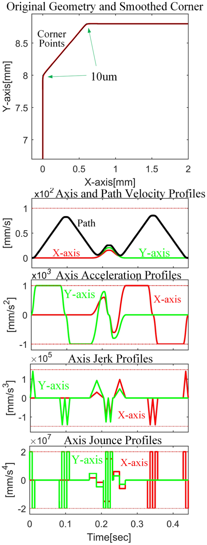
Motion planning along separated corners.

Figure 14.

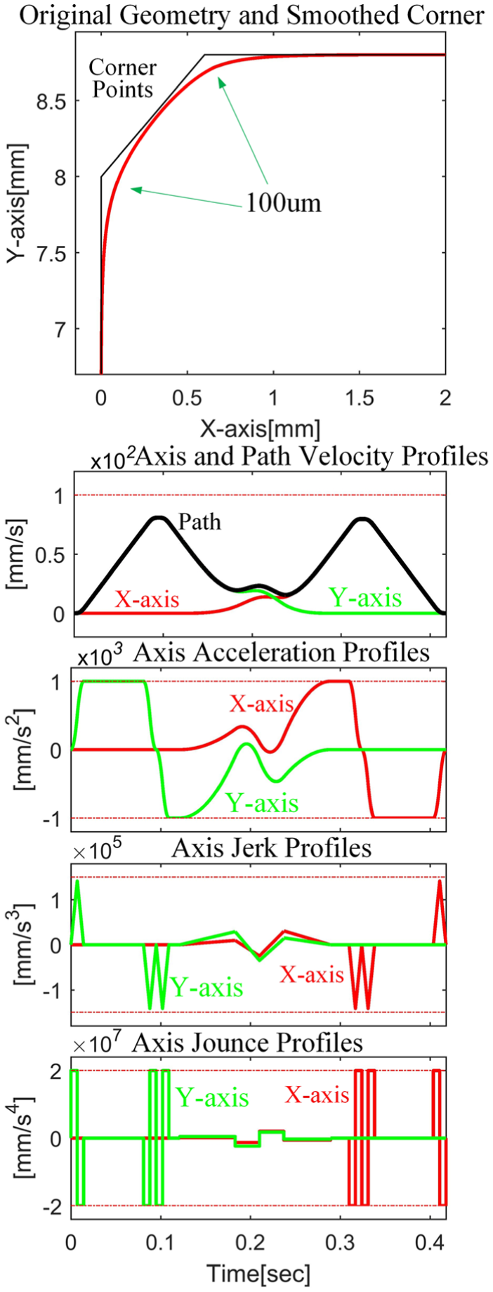
Motion planning along overlapping corners.

Experimental results

Experimental Cartesian X–Y motion system equipment is shown in Figure 15. Plane X–Y motion is guided by two linear motors. To maintain well position synchronization and path tracking, the servo amplifier is set to operate in torque (current) control mode. The feedback resolution of the linear encoder is 0.8 µm. The closed-loop sampling time of the servo system is 0.1 ms, and the position feedback bandwidth of X, Y axis is ω _n  = 25 Hz. The equipment used by the host computer is Windows 7 system, i5 2GHz clock chipset PC.

Figure 15.

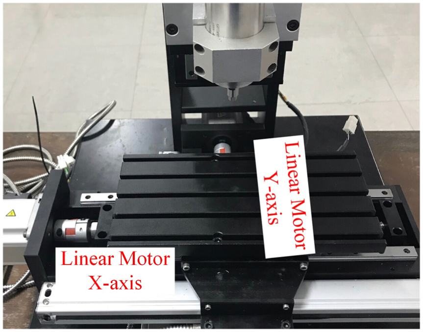
Experimental setup.

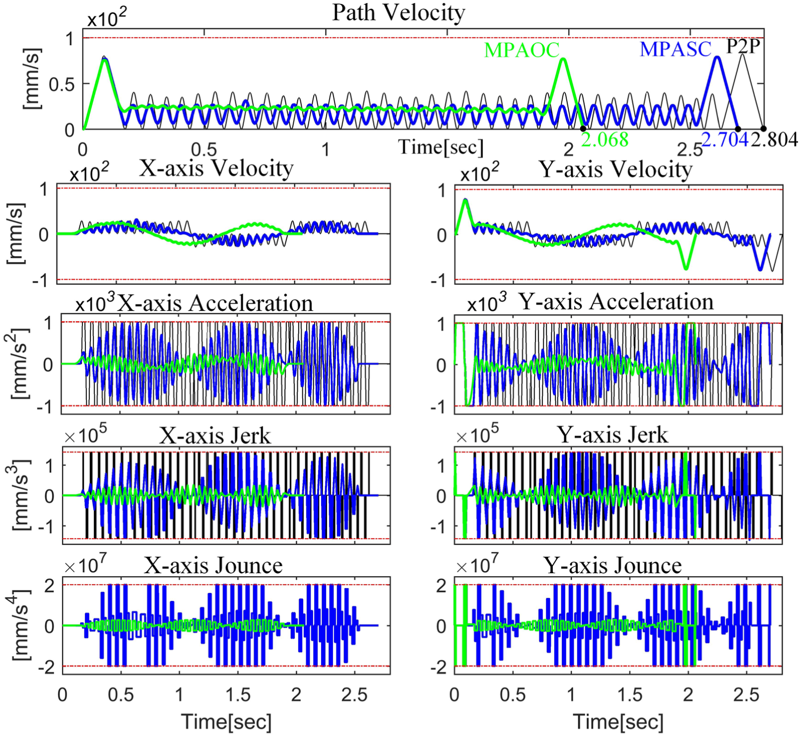
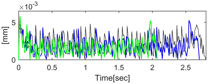
As shown in Figure 16, the helical tool-path has a total length of 51.43 mm and a total of 39 corner points, with the helical portion of the path being discrete as some short linear segments with an average length of 1.2 mm. P2P interpolation algorithm, MPASC algorithm and MPAOC algorithm are separately carried out on the helical path. The P2P interpolation algorithm requires the complete stop at each corner point, which is completely synchronized with the path of the G01 code. The maximum contour error of the MPASC is 3 µm and the maximum contour error of the MPAOC is 40 µm. The maximum feed velocity is set to 100 mm/s, the maximum acceleration is set to 1000 mm/s², and the maximum jounce is 2 × 10⁷ mm/s⁴. The motion profiles are demonstrated in Figure 17. Due to the short linear length, the feed motion between the corner profiles cannot reach the maximum feed velocity, and the MPASC must reduce the maximum contour error at the corners. In order to seek the optimal cornering velocity between linear segments, the maximum contour error is reduced by 0.02–0.08 µm from the specified value. The kinematics performances are shown in Figure 18. The P2P interpolation algorithm shows the longest machining time and the maximum speed fluctuations, while the jerk and acceleration values always reach the motion limit of the driver. The MPASC provides faster machining time, and it takes into account the jounce limit, so the acceleration curve reaches G² continuous. The MPAOC provides the least machining time, and the velocity curve tends to be steady with high values. At the same time, acceleration and jounce values are relatively small, the minimum load on the drive. Similarly, the acceleration curve reaches G² continuous. The experimental measurements of the contour errors are shown in Figure 19, and the larger contour errors for the three algorithms occur at the corners of the path. The total machining time, contour error, and calculation time are exhibited in Table 1. The total machining time of the MPASC algorithm is 3.6% higher than that of the P2P algorithm. The total machining time of the MPAOC algorithm is 26.2% higher than that of P2P algorithm. At the same time, the contour error performance of the three algorithms is basically the same. Finally, the computational load of P2P is the least, but its computational efficiency (computational time/machining time) is the lowest, which proves that MPASC and MPAOC algorithms are more suitable for modern NC systems.

Figure 16.

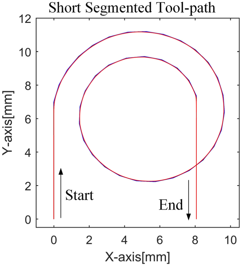
Motion planning along spiral tool-path.

Figure 17.

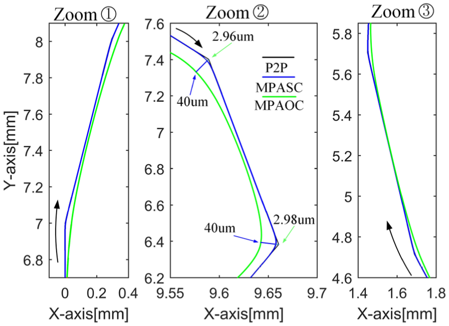
Tool-path and corner profiles.

Figure 18.

Kinematic profiles of algorithms.

Figure 19.

Measured contour errors in experiment.

Table 1.

Machining time and performance comparison in the helical tool-path.

Algorithms	Machining time (s)	Contour error		Computational time (s)	Unit computational effort
		RMS (µm)	MAX (µm)
P2P	2.804	2.43	5	0.317	0.113
MPASC	2.704	2.28	5.2	0.595	0.22
MPAOC	2.068	2.02	5.7	0.54	0.261

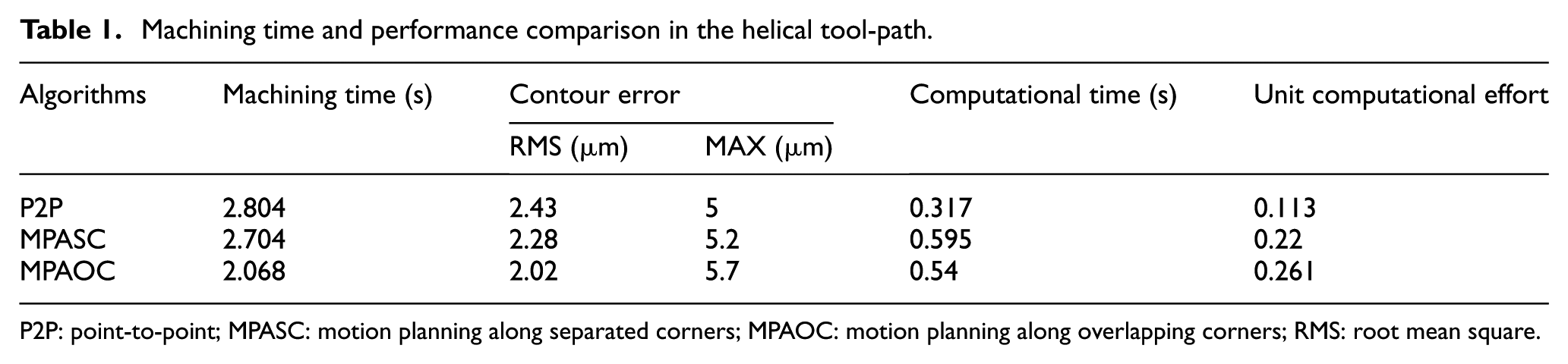
P2P: point-to-point; MPASC: motion planning along separated corners; MPAOC: motion planning along overlapping corners; RMS: root mean square.

Finally, experiments were performed on the more complex heart tool-path, as is shown in Figure 20. The length of the heart tool-path was 119 mm. Two hearts were discretized into short linear segments of 1.5 mm in length. Two short segments intersected to form a total of 50 corners. Some parameters are set up as follows: the maximum feed velocity is 150 mm/s, the maximum acceleration is 2000 mm/s², the maximum jounce is 1.5 × 10⁷ mm/s⁴, and the maximum contour error is 50 µm (Figure 21). Compared to P2P algorithm, NURBS interpolation algorithm ⁸ tests the performance of the proposed algorithm (Global). The performance is demonstrated in Figure 22. The P2P algorithm uses the longest machining time, and the velocity fluctuations become more intense as the acceleration limit increases. The acceleration and jerk reach the limit of the driver most of the time. The NURBS interpolation algorithm constructs the smooth acceleration tool-path for machining, resulting in faster cornering transition velocity and less velocity fluctuations. The load of the driver was less, and the machining time increased by 10.9% compared with the P2P algorithm. The proposed algorithm (Global) achieves the least machining time, which is nearly 18% faster than the P2P algorithm. It makes full use of the motion performance of the drive, the velocity fluctuation tends to be steady, and the acceleration curve reaches G² continuous. The experimental measurements of the contour errors are shown in Figure 23. After the increase in the speed and acceleration limit, the contour error of P2P increases obviously and the error fluctuation also increases. The errors of NURBS and Global algorithm are similar. The NURBS interpolation algorithm constructs complex parameter curve, so the computational time is the largest. The P2P algorithm does not need to consider the jounce limit, and there is no complicated calculation, so the computational time is the least. The Global algorithm does not need to find the optimal cornering transition velocity through deep iterative, greatly reducing the computational time, and its computational efficiency is improved by nearly 11% compared with the NURBS algorithm (Table 2).

Figure 20.

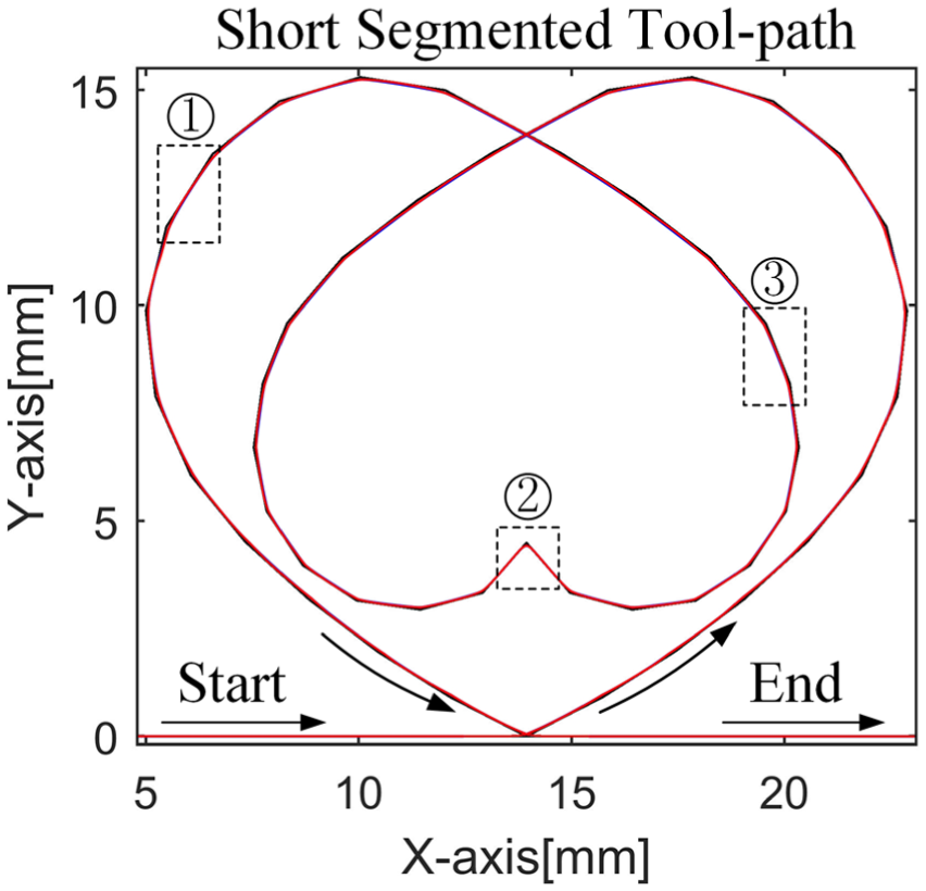
Motion planning along heart tool-path.

Figure 21.

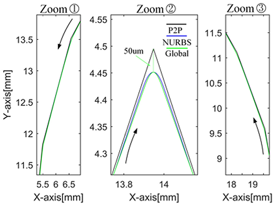
Tool-path and corner profiles.

Figure 22.

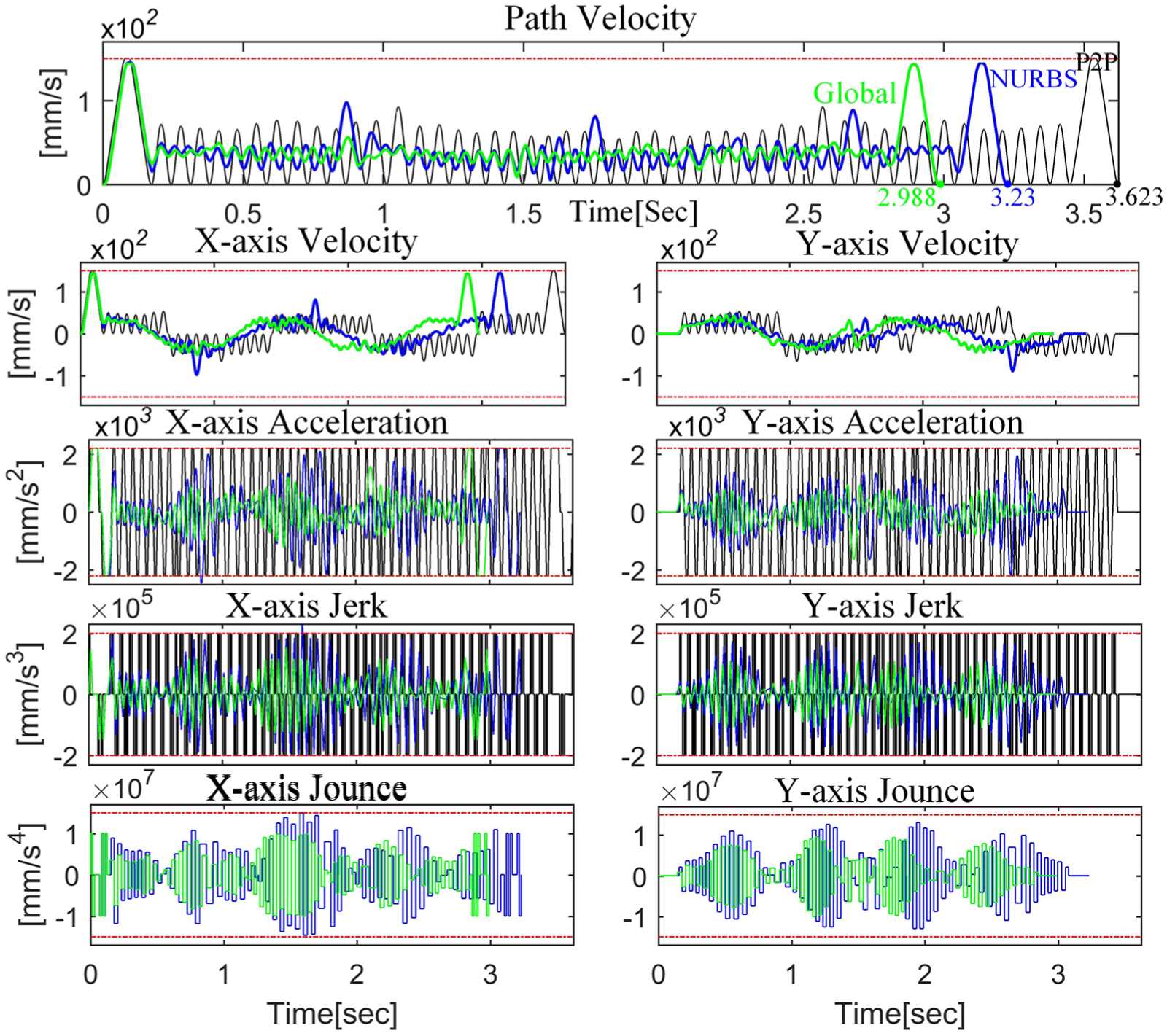
Kinematic profiles of algorithms.

Figure 23.

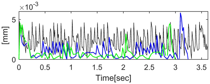
Measured contour errors in experiment.

Table 2.

Machining time and performance comparison in the heart tool-path.

Algorithms	Machining time (s)	Contour error		Computational time (s)	Unit computational effort
		RMS (µm)	MAX (µm)
P2P	3.623	3.83	5	0.47	0.13
NURBS	3.23	2.73	5.8	0.75	0.232
Global	2.988	2.36	4.5	0.62	0.207

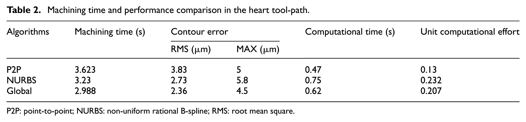
P2P: point-to-point; NURBS: non-uniform rational B-spline; RMS: root mean square.

Conclusion

In this article, the new interpolation algorithm is proposed for the global feed motion of continuous short linear segments. The algorithm interpolated the global tool-path based on jounce-limited acceleration curve to realize the balance between drive performance and machining time of the CNC system. At the corners of the machining path, the acceleration, velocity, and displacement boundary conditions are used to generate feed profile that can be used to precisely control cornering contour errors. A new kinematic look-ahead interpolation algorithm was developed for the short linear segments in the middle of the corners and the overlapping corner contours, which effectively stitched the feed motion between the corners, so the continuous feed motion and the G² continuous acceleration curve are achieved in the global tool-path. By contrasting the NURBS and P2P interpolation algorithms, the machining time is increased by 18% over the P2P algorithm when machining the tool-path with 50 corners. The computational efficiency was increased by 11% compared with the NURBS interpolation algorithm with the same tool-path. Experiments show that the proposed algorithm has application prospects in the producing and machining of complex parts.