Sage Journals: Discover world-class research

Abstract

A back-propagation neural network BP model and a genetic algorithm optimizing back-propagation neural network (GA-BP) model are proposed to predict the grinding forces produced during the creep-feed deep grinding of titanium matrix composites. These models consider quantitative and non-quantitative grinding parameters (e.g. up-grinding mode and down-grinding mode) as inputs. Comparative results show that the GA-BP model has better prediction accuracy (e.g. up to 95%) than the conventional regression model and the BP model. Specific grinding energy was calculated against the grinding parameters and grinding modes based on the grinding forces predicted by the GA-BP model.

Keywords

Grinding forces neural network Genetic algorithm optimizing back-propagation neural network specific grinding energy

Introduction

Creep-feed deep grinding (CFDG) is an effective method for machining difficult-to-cut materials. The highly nonlinear relationship between machine conditions and grinding forces in the CFDG process increases the unpredictability of some grinding phenomena.^1–5 Grinding force is crucial in the evaluation and monitoring of the machinability of workpiece materials; grinding force also determines surface finishing and specific grinding energy.^6–8 Therefore, a prediction model of grinding forces for CFDG should be developed to better understand the influence of processing parameters and predict and improve ground surface integrity and machining efficiency.^9–12

Several prediction models of grinding/cutting forces were established in recent years, which included numerical analytical models, regression models, and neural network models.^13–17 For example, Fuh and Wang¹³ applied the back-propagation (BP) neural networks to predict grinding forces; Li and Wang¹⁴ established a numerical simulation model to predict cutting forces during the machining of titanium alloy; Radhakrishnan and Nandan¹⁵ used regression and neural networks to predict milling forces. Previous studies showed that the analytical model can potentially monitor and calculate grinding/cutting forces in real time; however, the analytical model based on extensive amount of equations can be extremely complex because many factors need to be considered, such as material failure criteria and tool properties. Existing studies showed that the regression models have no advantages over neural network models in solving nonlinear problems.¹⁵ Different empirical formulas could be proposed in the process of building the regression model to calculate the up-grinding and down-grinding forces given the differences in grinding forces.¹⁶ Moreover, the prediction accuracy of the regression model is limited by experimental data. In particular, neural network has a high degree of parallelism, adaptive learning ability, and powerful nonlinear fitting ability. Neural network can handle complex nonlinear problems and has been widely used in artificial intelligence, pattern recognition, and signal processing. For example, Panda and Bhoi¹⁷ predicted the material removal rate in electro discharge machining using neural network model. Li et al.¹⁸ applied BP model to predict the mechanical properties of the shape memory alloy of porous NiTi manufactured by thermal explosion reaction. Qi et al.¹⁹ predicted surface roughness in belt polishing based on artificial neural network. Thus, the neural network model can potentially predict grinding forces based on limited experimental data with high accuracy.

At present, the BP neural network proposed by Rumelhart in the 1980s is the most widely used neural network with high prediction accuracy.²⁰ The BP neural network is based on the gradient descent method used to adjust the weights and thresholds and limit the mean square error (MSE) to the minimum. However, some inherent defects can be found in the BP algorithm, such as slow convergence and plunge into the local minimum. Some improved algorithms, such as particle swarm optimization (PSO) algorithm, hill-climbing algorithm, and genetic algorithm (GA), were proposed under such conditions to replace the BP algorithm for optimizing neural network to improve prediction accuracy.^21,22 Compared with other optimization algorithms, the GA was developed for several years and has become a mature and widely used algorithm. Various GA toolboxes were then developed, such as the GA optimization toolbox and the GA direct search toolbox, which facilitate the wide research application of GA.²³

GA provides a general framework for solving complex system optimization problems. GA is widely used in many disciplines, such as robotics, image processing, and combinatorial optimization. For example, Chan et al.²⁴ used GA to propose an approach for inventory-based multi-item lot-sizing problem. Lancaster and Cheng²⁵ applied GA to achieve the optimization of a hydro testing sequence in the construction of a tank farm. Recent studies successfully applied GA to optimize BP neural network and overcome the defects of BP algorithm.²¹ Sedki et al.²⁶ established the GA-BP model to predict daily rainfall runoff. Wang et al.²⁷ used GA-BP model to predict wind speed. GA is also widely used in mechanical engineering. For instance, Razfar et al.²⁸ applied neural network and GA to predict optimum damage and surface roughness in end milling glass fiber–reinforced plastics. Ma et al.²⁹ integrated artificial neural network with GA to achieve thermal error compensation of the shaft in a high-speed spindle system.

On the basis of these findings, the present study proposes two neural network models, namely, the BP model and the GA-BP model, by simultaneously applying quantitative and non-quantitative parameters (e.g. up-grinding and down-grinding) as inputs to predict grinding forces in the CFDG of titanium matrix composites. A regression prediction model is also applied as comparison to investigate prediction accuracy. Specific grinding energy is calculated based on the grinding forces predicted using the GA-BP model. This approach provides a basis for optimizing grinding parameters and grinding modes.

Methodology

Regression model algorithm

The grinding forces in CFDG operations are usually affected by many factors. Grinding parameters are the key grinding forces when the workpiece materials, grinding wheel, and cooling condition are given. The grinding forces would change if different grinding modes (e.g. up-grinding or down-grinding) are applied.^15,24 Therefore, the present study proposes empirical formulas based on the regression algorithm to predict grinding force in up-grinding and down-grinding conditions. The grinding forces (including the normal grinding force and the tangential grinding force) can be expressed as¹⁵

F = k_{1} (v_{s})^{d_{1}} (v_{w})^{d_{2}} (a_{p})^{d_{3}}

(1)

where F is the grinding force, k₁ is regression coefficient, v_s is abrasive wheel speed, v_w is workpiece infeed speed, a_p is the depth of cut; d₁, d₂, and d₃ are the correlation coefficients of variables, respectively.

Multiple linear equations can be obtained by taking the logarithms simultaneously on both sides of equation (1) as follows

y = d_{0} + d_{1} x_{1} + d_{2} x_{2} + d_{3} x_{3}

(2)

where y = ln F; d₀ = ln k₁; x₁ = ln v_s; x₂ = ln v_w; x₃ = ln a_p.

According to the regression algorithm, the coefficients of equation (2) are determined based on “training data.” The regression model is established.

BP algorithm

The structure of the BP model is schematically displayed in Figure 1. The grinding parameters (e.g. abrasive wheel speed v_s, depth of cut a_p and workpiece infeed speed v_w) and the grinding mode (up-grinding and down-grinding) are used as input parameters. The up-grinding mode is quantitatively expressed as −1, whereas the down-grinding mode is defined as 1. Normal grinding force F_n and tangential grinding force F_t are utilized as output parameters.

Figure 1.

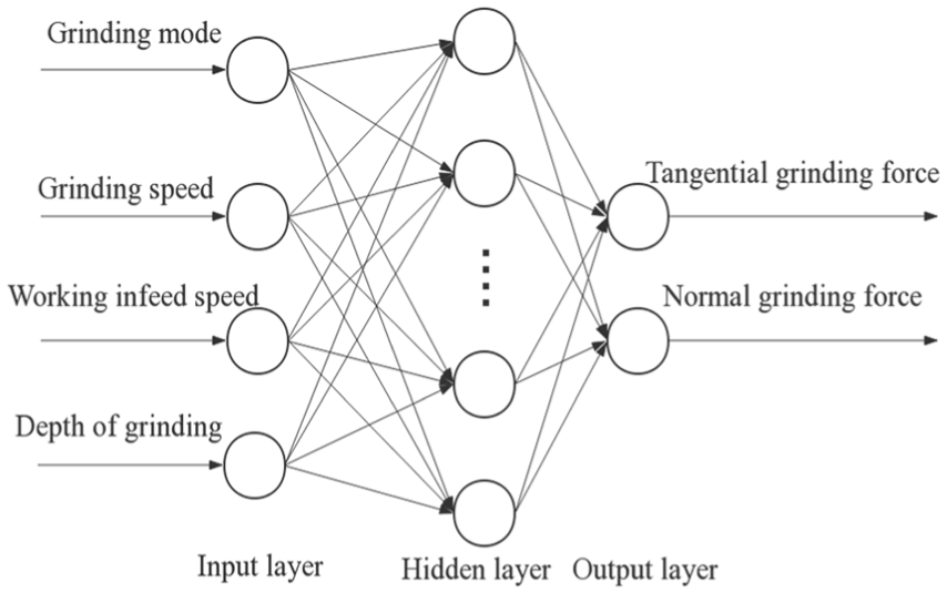
Structure of the applied BP model.

The traditional BP algorithm can be divided into two steps. The first step is forward transmission, whereas the second one is error back propagation:

Forward transmission: The output of the BP neural network can be represented as vector Y = (y₁, y₂,…, y_n). The MSE function between the output values and the expected outputs can then be described as

E = \frac{1}{n} \sum_{k = 1}^{n} {(y_{k} - d_{k})}^{2}

(3)

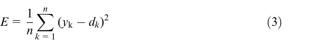
where d_k is an expected value of network output.

Error back propagation: The weights and thresholds of the BP neural network are updated using the gradient descent algorithm to minimize MSE.²⁰

However, the BP algorithm is often slow in converging and plunging into the local minimum. To overcome these problems and improve prediction accuracy, GA was developed and applied to optimize initial weights and thresholds.

GA

GA is derived from Holland’s work in the 1960s.²² GA is a precise method of searching for the global optimal solution by imitating natural evolution process. Figure 2 shows the procedure of the GA-BP model.

Figure 2.

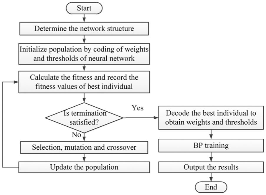
Flowchart of GA.

First, a single gene, which is also called an individual, can be obtained by encoding initial weights and thresholds. An individual consists of four parts, namely, hidden layer connection weights, hidden layer thresholds, output layer connection weights, and output layer thresholds, which are performed with the following binary code

x = c_{1} c_{2} \dots c_{b}

(4)

where x stands for an individual and c₁c₂…c_b is a binary number, wherein c_i = (1, 2,…, b) is 0 or 1.

A population consists of a certain number of individuals, which could be represented as vector X = (x₁, x₂,…, x_i). The reciprocal of the MSE function is determined as fitness function to demonstrate the merits and demerits of the individuals in the population, which is expressed as

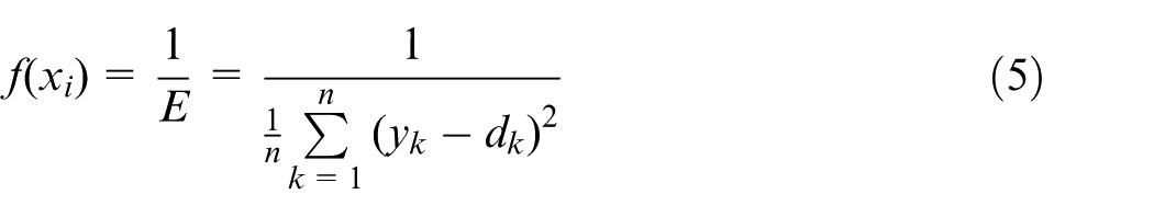
f (x_{i}) = \frac{1}{E} = \frac{1}{\frac{1}{n} \sum_{k = 1}^{n} {(y_{k} - d_{k})}^{2}}

(5)

where y_k is the output value of the neural network determined by an individual x_i; d_k is the expected output value.

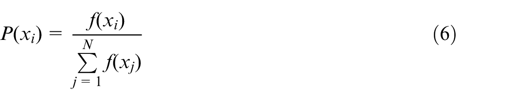
A new population X′ would be formed when the termination conditions of GA, that is, the fitness value does not meet the requirement or the maximum genetic algebra, are not satisfied. The individuals in the new population are obtained by the operations of selection, crossover, and mutation. A higher fitness individual is more likely to be selected. Individual selection probability can be expressed as²⁰

P (x_{i}) = \frac{f (x_{i})}{\sum_{j = 1}^{N} f (x_{j})}

(6)

In the process of generating offspring, the performance of mutation is followed by probability P_m and crossover with probability P_c. The GA ends until the termination condition is reached.

Grinding experiments details

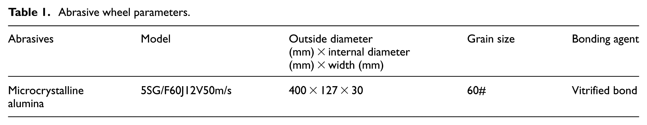
CFDG experiments of titanium matrix composites were conducted on grinding machine model BLOHM PROFIMAT MT-408. The maximum speed of abrasive wheel could reach 175 m/s when the diameter of the largest wheel is 400 mm and the speed of the highest workpiece infeed is 30 m/min. A microcrystalline corundum abrasive wheel was employed and its parameters are listed in Table 1. The applied titanium matrix composite is a typical difficult-to-cut material, wherein the dominating reinforcements are TiC particles.³⁰

Table 1.

Abrasive wheel parameters.

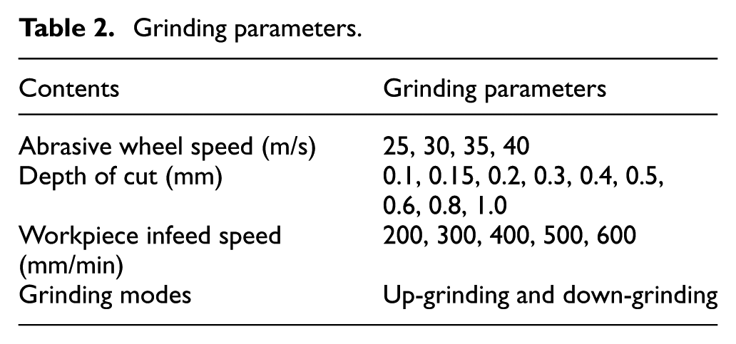
Abrasives	Model	Outside diameter(mm) × internal diameter(mm) × width (mm)	Grain size	Bonding agent
Microcrystallinealumina	5SG/F60J12V50m/s	400 × 127 × 30	60#	Vitrified bond

Single-factor CFDG experiments were performed on workpiece samples with 30 mm length, 5 mm width, and 20 mm height. CFDG operations were conducted with the grinding parameters (v_s, v_w, and a_p) as variables in different grinding modes (up-grinding or down-grinding). The experimental conditions are listed in Table 2. The grinding force in the up-grinding mode was measured by four direction piezoelectric dynamometer modeled KISTLER 9272, as shown in Figure 3. In terms of measuring the down-grinding force, the speed direction of the workpiece infeed was opposite to the workpiece infeed speed direction, as shown in Figure 3.

Table 2.

Grinding parameters.

Contents	Grinding parameters
Abrasive wheel speed (m/s)	25, 30, 35, 40
Depth of cut (mm)	0.1, 0.15, 0.2, 0.3, 0.4, 0.5,0.6, 0.8, 1.0
Workpiece infeed speed(mm/min)	200, 300, 400, 500, 600
Grinding modes	Up-grinding and down-grinding

Figure 3.

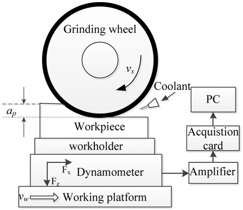
Measurement system of up-grinding force in CFDG experiment.

The grinding forces were measured five times under the same grinding parameters. The average values in the stable fluctuation stage were obtained in the grinding process. In the creep grinding process, normal grinding forces F_n and tangential grinding forces F_t are described as³¹

F_{n} = F_{z} \cos θ - F_{x} \sin θ

(7)

F_{t} = F_{z} \sin θ + F_{x} \cos θ

(8)

where F_z is the measured vertical force, F_x is the measured horizontal force, and θ is the angle between the vertical force perpendicular to the workpiece and the normal force vector acting on the grinding zone.

Results and discussion

Grinding forces obtained in the experiments

As shown in Table 3, the experimental results of grinding forces obtained in the present work were divided into the training group (e.g. Samples no. 4, no. 7, no. 13, no. 18, no. 21, no. 24, no. 27, no. 32) and the testing group to validate model accuracy (rest of the samples).

Table 3.

Grinding forces obtained with different grinding parameters.

Sample no.	Grinding mode	Abrasive wheelspeed v_s (m/s)	Workpiece infeedspeed v_w (mm/min)	Depth of cut a_p (mm)	Normal grindingforce F_n (N)	Tangential grindingforce F_t (N)
1	1	25	300	0.3	150.5	65.5
2	−1	25	300	0.3	161	63
3	1	30	300	0.3	130.5	49.5
5	1	35	300	0.3	162	51
6	−1	35	300	0.3	130	43
8	−1	40	300	0.3	130	39
9	1	20	300	0.1	52.65	25.5
10	−1	20	300	0.1	45.01	15.31
11	1	20	300	0.15	67.93	37.96
12	−1	20	300	0.15	69.04	33.3
14	−1	20	300	0.2	152.2	57.16
15	1	20	300	0.4	233	86.8
16	−1	20	300	0.4	201	73
17	1	20	300	0.5	270	96
19	1	20	300	0.6	291	104
20	−1	20	300	0.6	266	99.7
22	−1	20	300	0.8	303	116
23	1	20	300	1	455	143
25	1	20	200	0.3	165.5	63.7
26	−1	20	200	0.3	154.5	73
28	−1	20	300	0.3	181	62.5
29	1	20	400	0.3	206	86
30	−1	20	400	0.3	222	81
31	1	20	500	0.3	217	88
33	1	20	600	0.3	255	98.5
34	−1	20	600	0.3	218	86
4	−1	30	300	0.3	147	50
7	1	40	300	0.3	161	47
13	1	20	300	0.2	99.43	49.51
18	−1	20	300	0.5	232	82
21	1	20	300	0.8	386	126
24	−1	20	300	1	341	137
27	1	20	300	0.3	186.5	73.5
32	−1	20	500	0.3	206	79

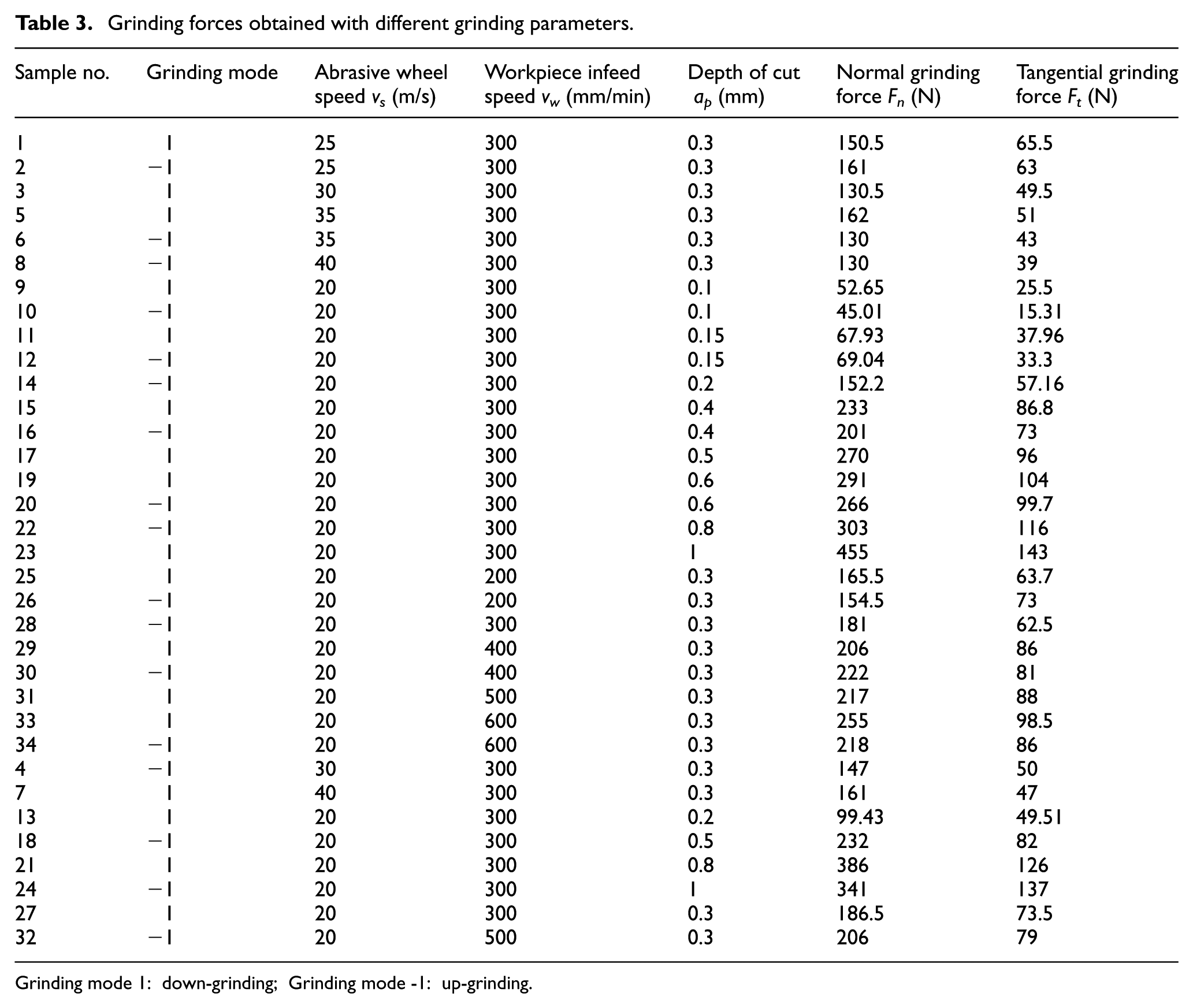
Grinding mode 1: down-grinding; Grinding mode -1: up-grinding.

The training samples were used to establish the empirical formula based on the regression algorithm, which are described as follows:

Empirical formula for the up-grinding mode

F_{n} = 88.6326 {v_{s}}^{- 0.2966} {v_{w}}^{0.4483} {a_{p}}^{0.8999}

(9)

F_{t} = 189.3127 {v_{s}}^{- 0.6285} {v_{w}}^{0.3223} {a_{p}}^{0.8861}

(10)

Empirical formula for the down-grinding mode

F_{n} = 45.6225 {v_{s}}^{- 0.1966} {v_{w}}^{0.5307} {a_{p}}^{0.9725}

(11)

F_{t} = 42.2879 {v_{s}}^{- 0.5209} {v_{w}}^{0.5098} {a_{p}}^{0.7410}

(12)

To accelerate the convergence speed and reduce the training time, experimental data were normalized in the interval of [–1, 1], which was calculated according to the following equations

x' = \frac{x - x_{mid}}{\frac{1}{2} (x_{max} - x_{min})}

(13)

x_{mid} = \frac{x_{min} + x_{max}}{2}

(14)

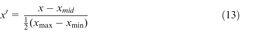
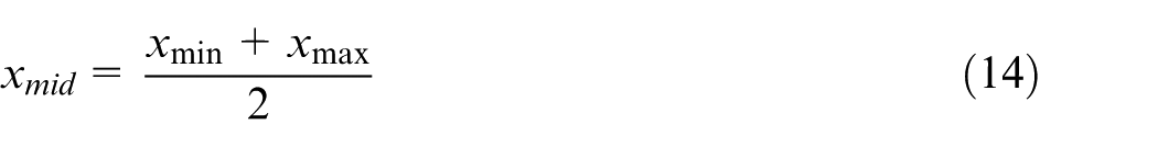
where x is the original value and x_min and x_max are the minimum value and maximum value of original data, respectively.

Many factors can affect prediction accuracy in the process of establishing the BP model. These factors mainly include activation function, number of hidden layers, and number of neurons in hidden layers. In general, the sigmoid function is adopted as activation function because its derivatives are continuous and derivable. Therefore, the active function of the hidden layer is determined as the tan-sigmoid function and the active function of the output layer is determined as purelin function.³² In this BP model, the number of hidden layers is 1 because the number of neurons in the input and output layers are small; the number of neurons in hidden layer can be determined by the following formula³³

m = \sqrt{n + l} + α

(15)

where n and l are the number of neurons in the input and output layers and α is between 0 and 10. Therefore, the value of m ranges from 3 to 13.

The number of neurons in the hidden layer varies from 3 to 13 to obtain the best structures. The best structure is evaluated by the MSE, which is shown in Figure 4.

Figure 4.

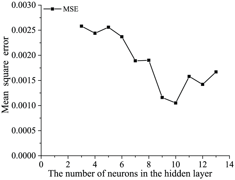
Mean square error of BP neural network with different numbers of neurons in the hidden layer.

The number of neurons in the hidden layer is determined to be 10, with four input neurons and two output neurons. The structure is determined as 4-10-2. To avoid over-fitting, the third termination conditions are proposed when the MSE of the BP neural network does not decrease for six successive iterations.

The GA-BP model was established in the present study. The structure of the GA-BP model was similar to that of the model. The parameters of population size, genetic algebra, crossover probability, mutation probability, and generation gap of GA have some influences on the accuracy and convergence rate of neural networks. In general, the number of individuals in the population is in the range of [20, 100]. The termination evolution algebra takes between [100, 500]; the crossover probability is usually at the area of [0.4, 0.99]; the mutation probability is usually at the area of [0.0001, 0.1], and each weight or threshold will be encoded into binary digits with 10 digits.^34,35 Table 4 lists the parameters of the GA-BP model.

Table 4.

Selection of parameters in the GA-BP model.

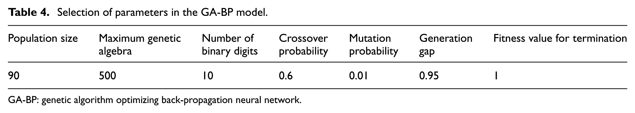
Population size	Maximum geneticalgebra	Number ofbinary digits	Crossoverprobability	Mutationprobability	Generationgap	Fitness value for termination
90	500	10	0.6	0.01	0.95	1

GA-BP: genetic algorithm optimizing back-propagation neural network.

The training samples are trained on GA-BP model and the fitness values of the optimal individual in each population are recorded as shown in Figure 5. Fitness value initially increases rapidly with the increase of genetic algebra. When the genetic algebra reaches 400, the fitness value remains constant at nearly 0.85. Therefore, genetic algebra can be appropriately set to 500.

Figure 5.

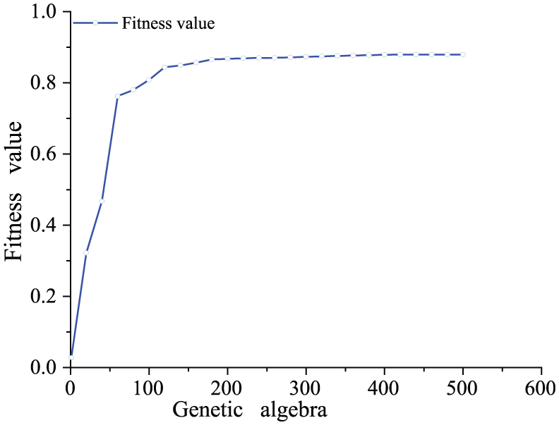
The best fitness value in each generation.

Comparative analysis of grinding force based on different prediction models

In order to assess the performance of the three prediction models, the following indexes are used: absolute percentage error (APE), mean absolute percentage error (MAPE), and coefficient of linear fitting determination (R²)

A P E = \frac{| {T^{'}}_{i} - T_{i} |}{T_{i}} \times 100 %

(16)

M A P E = \frac{1}{n} \sum_{i = 1}^{n} | \frac{T'_{i} - T_{i}}{T_{i}} | \times 100 %

(17)

R^{2} = 1 - \frac{\sum_{i = 1}^{n} {({T'}_{i} - T_{i})}^{2}}{\sum_{i = 1}^{n} {(T_{i} - T)}^{2}}

(18)

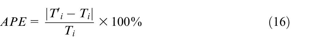
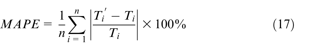
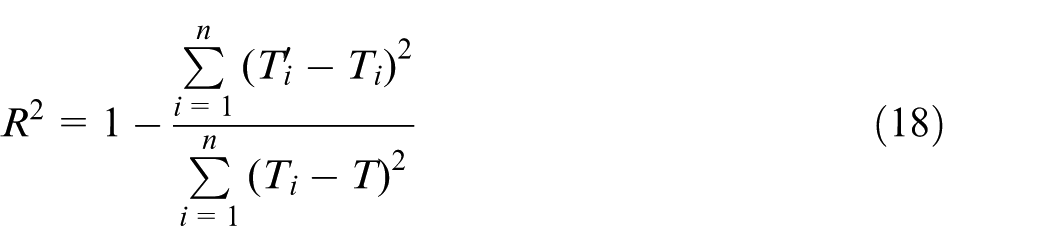
where n is the number of samples; T_i are the experimental results; ${T_{i}}^{'}$ are the predicted results; T is the mean value of ${T_{i}}^{'}$ .

The predicted results of the grinding forces are provided in Tables 5 and 6 and Figure 6, respectively. Prediction data I, II, and III are obtained by the regression model, the BP model, and the GA-BP model, respectively.

Table 5.

Normal grinding force.

Sample no.	Experimentaldata (N)	Predicteddata I (N)	APE (%)	Predicteddata II (N)	APE (%)	Predicteddata III (N)	APE (%)
4	147	141.0698	4.03	133.2948	9.32	139.9464	4.8
7	161	141.3588	12.2	204.979	27.32	177.0402	9.96
13	99.43	109.2085	9.83	97.9287	1.51	101.5344	2.12
18	232	251.9443	8.6	261.3476	12.65	247.9822	6.89
21	386	420.494	8.94	354.3363	8.2	392.301	1.63
24	341	470.1121	37.86	407.8613	19.61	340.8884	0.03
27	186.5	161.9964	13.14	173.1639	7.15	164.3477	11.88
32	206	200.0404	2.89	195.2671	5.21	206.753	0.37

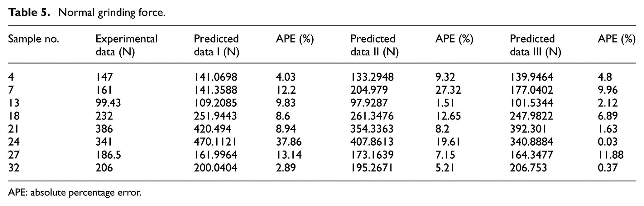
APE: absolute percentage error.

Table 6.

Tangential grinding force.

Sample no.	Experimentaldata (N)	Predicteddata I (N)	APE (%)	Predicteddata II (N)	APE (%)	Predicteddata III (N)	APE (%)
4	50	48.2906	3.42	51.4508	8.78	50.6561	1.31
7	47	46.4714	1.12	55.4331	17.94	49.4876	5.29
13	49.51	49.3751	0.27	47.0972	4.87	51.43	3.88
18	82	97.9751	19.48	96.7041	17.93	92.2556	12.51
21	126	137.9224	9.46	118.0273	6.33	124.5028	1.19
24	137	181.075	32.17	149.4766	9.11	135.9278	0.78
27	73.5	66.6794	9.28	69.7265	5.13	71.3039	2.99
32	79	73.4577	7.02	74.2155	6.06	81.4657	3.12

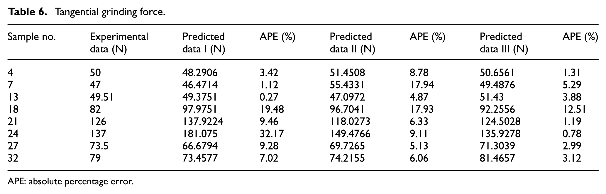
APE: absolute percentage error.

Figure 6.

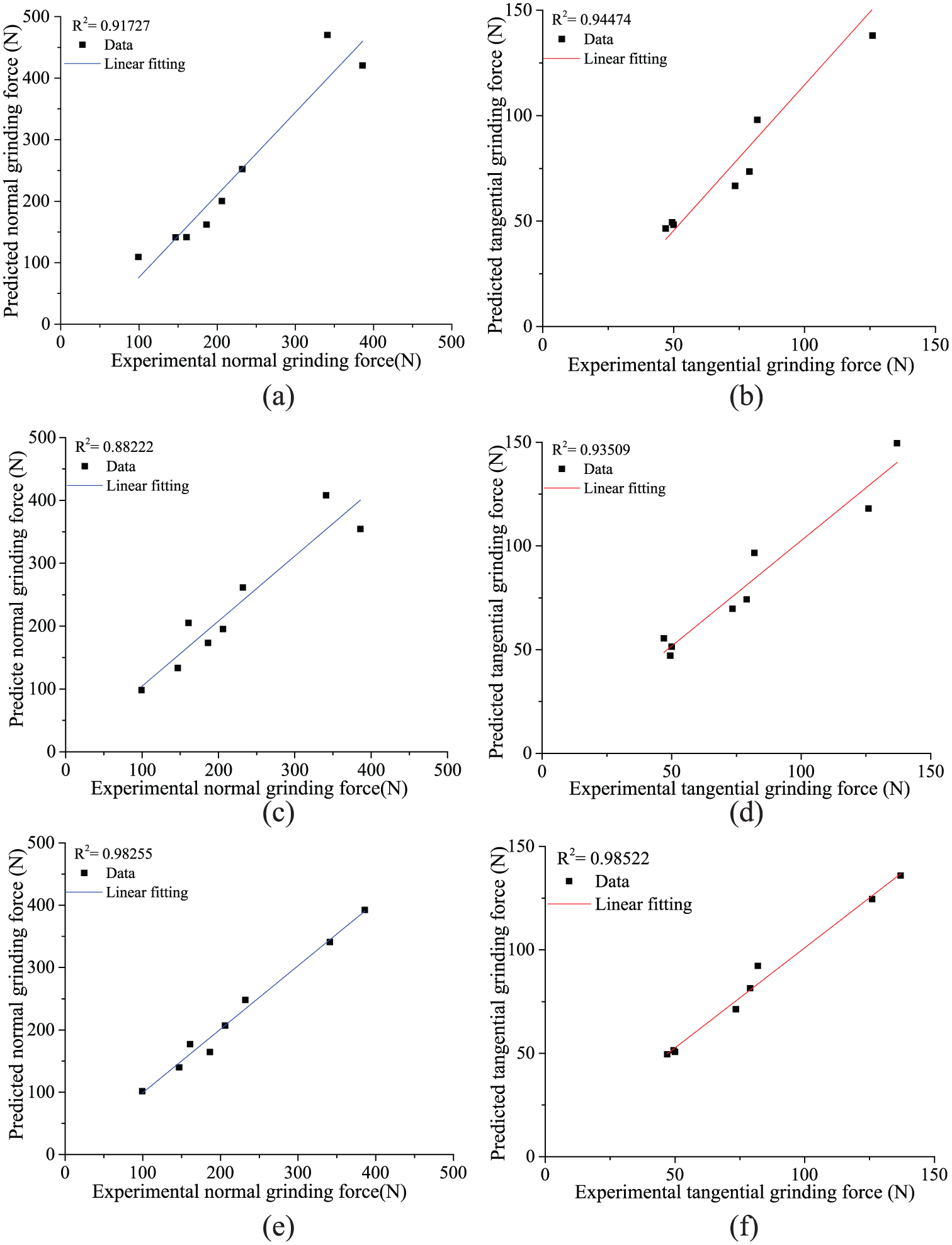
Comparison of predicted results with experimental results: (a), (c), and (e) are the correlation between the predicted normal grinding force and experimental grinding force for the regression model, BP model, and the GA-BP model, respectively; (b), (d), and (f) are the correlation between the predicted tangential grinding force and experimental tangential force for regression model, BP model, and GA-BP model, respectively.

The indexes MAPE, R², and prediction accuracy of the predicted results of the three above mentioned models are listed in Table 7.

Table 7.

Evaluation indexes of the predicted results.

Models	Predicted normal grinding force		Predicted tangential grinding force		Prediction accuracy
Models	MAPE (%)	R ²	MAPE (%)	R ²	(%)
Regression model	12.19	0.9172	10.28	0.94474	88.765
BP model	9.32	0.92816	8.78	0.92889	90.95
GA-BP model	4.71	0.98255	3.88	0.98522	95.705

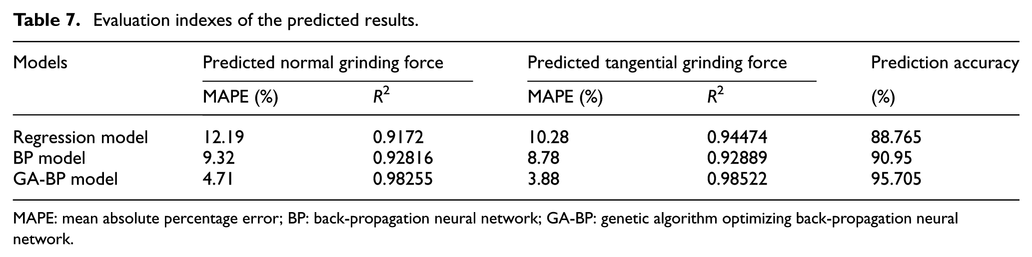
MAPE: mean absolute percentage error; BP: back-propagation neural network; GA-BP: genetic algorithm optimizing back-propagation neural network.

The predicted results of the three models and its APE are displayed in Figure 7. The predicted results based on the GA-BP model are more consistent with the experimental results than the other two models. The normal and tangential grinding force evaluation indexes R² of GA-BP model are higher than 0.98, which is higher than that of the other two models at 0.92, 0.94, 0.93, and 0.93. In particular, the prediction accuracy of the grinding forces predicted by the GA-BP model is higher than 95%, which is nearly 7% higher than that of the regression model and nearly 5% higher than that of the BP model. These results are shown in Table 7. The present study infers that the GA-BP neural network model has a higher prediction accuracy than the other two models, which has better potential in optimizing grinding parameters and grinding modes.

Figure 7.

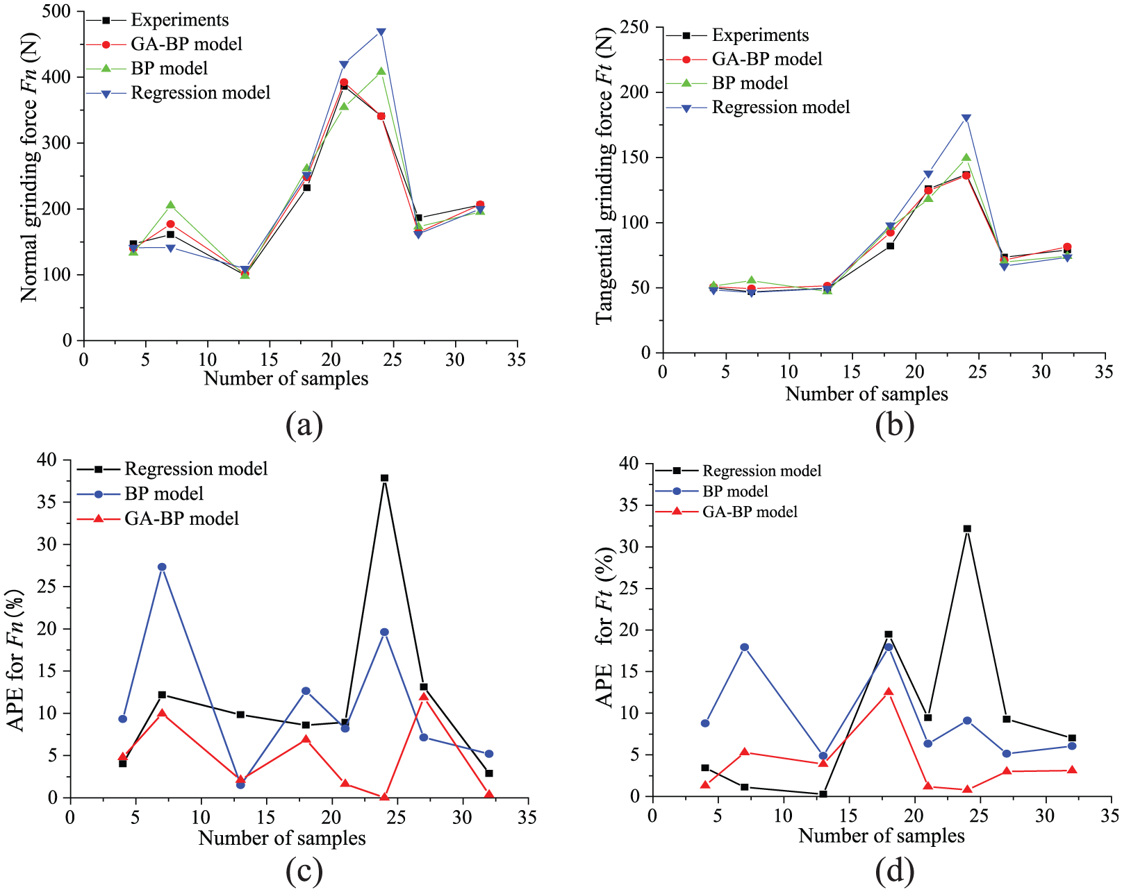
Comparison of predicted results based on different models: (a) and (b) are the comparison of predicted results and experimental results; (c) and (d) are the APE of the predicted results.

Specific grinding energy based on the predicted grinding forces

The specific grinding energy is defined as the amount of energy consumed by grinding a unit volume of material, which is a fundamental parameter to optimizing the grinding conditions.³⁰ The specific grinding energy can be obtained from the following relationship³⁶

e_{s} = \frac{F_{t} v_{s}}{v_{w} a_{p} b}

(19)

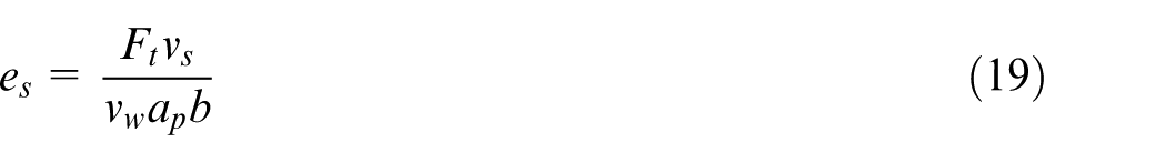
where b is the width of the workpiece.

Figure 8 shows the specific grinding energy (e_s) calculated based on the predicted grinding forces using GA-BP model. Teicher et al. reported that the thermal damage to workpiece always corresponds to high specific grinding energy.^37,38 Malkin and Guo³⁹ indicated the presence of a critical specific energy value that causes thermal damage to the workpiece; they also reported that a higher material removal rate was accompanied by a low specific energy of about 20–25 J/mm³ during grinding of brittle material, such as silicon nitride ceramics. Previous studies showed that the workpiece can be well machined when the specific energy of grinding titanium matrix composites ranges from about 40–90 J/mm³.^30,31 As shown in Figure 8, the specific grinding energy drops rapidly with the increase of the depth of cut when the depth of cut is lower than 0.5 mm. However, the specific grinding energy generally remains constant when the depth of cut is higher than 0.5 mm, which corresponds to the size effects in grinding. When the abrasive wheel speed and workpiece infeed speed are constant, the undeformed chip thickness increases with the increase of depth of cut. The number of effective abrasive grains that remove the workpiece material also increases. Therefore, the specific grinding energy drops with the increase of the depth of cut. This phenomenon reveals the inverse relationship between specific grinding energy and undeformed chip thickness.⁴⁰ In particular, the specific grinding energy produced in up-grinding mode is slightly smaller than that in the down-grinding mode under identical grinding parameters. Therefore, the optimum grinding parameters and modes in CFDG of titanium matrix composites are determined when low thermal damage and high grinding efficiency are required at below the critical value, that is, 90 J/mm³ of the specific grinding energy, as shown in Figure 8. The selection of machining parameters should also consider the grinding temperature and the surface quality of the workpiece, which will be further studied in the future.

Figure 8.

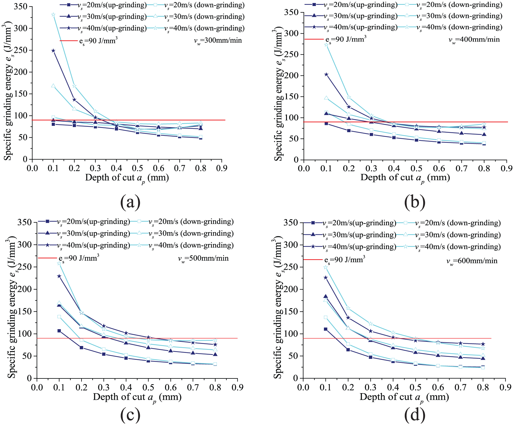
Influence of grinding parameters on the specific grinding energy calculated: (a) v_w = 300 mm/min, (b) v_w = 400 mm/min, (c) v_w = 500 mm/min, and (d) v_w = 600 mm/min.

Conclusion

Two neural network models, namely, BP model and GA-BP model, are established by simultaneously introducing quantitative and non-quantitative parameters (e.g. up-grinding mode and down-grinding mode) as inputs.

The GA-BP model has a higher value of prediction accuracy (e.g. up to 95%) than the accuracy of prediction results of the regression model (e.g. 88.7%) and that of the BP model (e.g. 90.9%). Therefore, the GA-BP model has generally better potential in predicting grinding forces.

The variation tendency of specific grinding energy versus the grinding parameters is obtained based on the predicted grinding force.

Footnotes

Declaration of conflicting interests

The author(s) declared no potential conflicts of interest with respect to the research, authorship, and/or publication of this article.

Funding

The author(s) disclosed receipt of the following financial support for the research, authorship, and/or publication of this article: The authors gratefully acknowledge the financial support for this work from the National Science Foundation of China (No. 51775275 and No. 5137 5235), the Fundamental Research Fund for the Central University (No. NE2014103), and the Foundation of Graduate Innovation Center in NUAA (No. kfjj2017 0527).

ORCID iD

Wen-Feng Ding

References

Bastawros

Chandra

Experimental and modeling characterization of wear and life expectancy of electroplated CBN grinding wheels. Int J Mach Tools Manuf 2017; 121: 70–80.

Zhu

Ding

et al . Investigation on stress distribution and wear behavior of brazed polycrystalline cubic boron nitride superabrasive grains: numerical simulation and experimental study. Wear 2017; 376: 1234–1244.

Dai

Ding

et al . Influence of grain wear on material removal behavior during grinding nickel-based superalloy with a single diamond grain. Int J Mach Tools Manuf 2017; 113: 49–58.

Ding

Dai

et al . Grinding performance of textured monolayer CBN wheels: undeformed chip thickness nonuniformity modeling and ground surface topography prediction. Int J Mach Tools Manuf 2017; 122: 66–80.

Wang

Fuh

KH.

The workpiece temperature, fluid cooling effectiveness and burning threshold of grinding energy in creep feed grinding. Proc IMechE Part B: J Engineering Manufacture 1998; 212(5): 383–391.

Lin

et al . Experimental studies on grinding forces and force ratio of the unsteady-state grinding technique. J Mater Proc Tech 2002; 129(1): 76–80.

Lee

Kim

Baek

et al . A study on tool condition monitoring and diagnosis of micro-grinding process based on feature extraction from force data. Proc IMechE Part B: J Engineering Manufacture 2014; 229(8): 1472–1478.

Sieniawski

Nadolny

Experimental study into the grinding force in surface grinding of steel CrV12 utilizing a zonal centrifugal coolant provision system. Proc IMechE Part B: J Engineering Manufacture 2016; 232: 394–403.

Zeng

Liu

et al . Investigation into grindability of a superalloy and effects of grinding parameters on its surface integrity. Proc IMechE Part B: J Engineering Manufacture 2015; 229(2): 238–250.

10.

Soo

Hood

Lannette

et al . Creep feed grinding of burn-resistant titanium (BuRTi) using superabrasive wheels. Int J Adv Manuf Tech 2011; 539(9): 1019–1026.

11.

Hood

Lechner

Aspinwall

et al . Creep feed grinding of gamma titanium aluminide and burn resistant titanium alloys using SiC abrasive. Int J Mach Tools Manuf 2007; 47(9): 1486–1492.

12.

Asplund

Bastawros

et al . Performance and modeling of paired polishing process. Int J Mach Tools Manuf 2016; 109: 49–57.

13.

Fuh

Wang

SB.

Force modeling and forecasting in creep feed grinding using improved BP neural network. Int J Mach Tools Manuf 1997; 37(8): 1167–1178.

14.

Wang

Numerical simulation and prediction of cutting force in turning of titanium alloy. Adv Mater Res 2012; 580: 63–66.

15.

Radhakrishnan

Nandan

Milling force prediction using regression and neural networks. J Intel Manuf 2005; 16(1): 93–102.

16.

Wager

DY.

Influence of up-grinding and down-grinding on the contact zone. CIRP Ann 1991; 40(1): 323–32616.

17.

Panda

Bhoi

RK.

Artificial neural network prediction of material removal rate in electro discharge machining. Mater Manuf Proc 2005; 20(4): 645–672.

18.

et al . BP neural network prediction of the mechanical properties of porous NiTi shape memory alloy prepared by thermal explosion reaction. Mater Sci Eng A 2006; 419(1): 214–217.

19.

Zhang

et al . Modeling and prediction of surface roughness in belt polishing based on artificial neural network. Proc IMechE Part B: J Engineering Manufacture 2018; 232(12): 2154–2163.

20.

Cheng

Shi

et al . Brief introduction of back propagation BP neural network algorithm and its improvement. Adv Comp Sci Inf Eng 2012; 169: 553–558.

21.

Ding

JZ.

An optimizing BP neural network algorithm based on genetic algorithm. Artif Intell Rev 2011; 36(2): 153–162.

22.

Haupt

RL.

An introduction to genetic algorithms for electromagnetics. IEEE Antenn Propag M 1995; 37(2): 7–15.

23.

Abramson

MA.

Genetic algorithm and direct search toolbox user’s guide. Natick, MA: MathWorks, 2007.

24.

Chan

FTS

Tibrewal

Prakash

et al . A biased random key genetic algorithm approach for inventory-based multi-item lot-sizing problem. Proc IMechE Part B: J Engineering Manufacture 2015; 229(1): 157–171.

25.

Lancaster

Cheng

Optimization of the hydrotesting sequence in tank farm construction using an adaptive genetic algorithm with stochastic preferential logic. Proc IMechE Part B: J Engineering Manufacture 2008; 222(2): 367–371.

26.

Sedki

Ouazar

El Mazoudi

Evolving neural network using real coded genetic algorithm for daily rainfall–runoff forecasting. Exp Syst Appl 2009; 36(3): 4523–4527.

27.

Wang

Zhang

et al . Wind speed forecasting based on the hybrid ensemble empirical mode decomposition and GA-BP neural network method. Renew Energ 2016; 94: 629–636.

28.

Razfar

Zadeh

MRZ

. Optimum damage and surface roughness prediction in end milling glass fibre-reinforced plastics, using neural network and genetic algorithm. Proc IMechE Part B: J Engineering Manufacture 2009; 223(6): 653–664.

29.

Zhao

Mei

et al . Thermal error compensation based on genetic algorithm and artificial neural network of the shaft in the high-speed spindle system. Proc IMechE Part B: J Engineering Manufacture 2016; 231(5): 753–767.

30.

Ding

Zhao

et al . Grinding behavior and surface appearance of TiCp+ TiBw/Ti-6Al-4V titanium matrix composites. Chi J Aeronautics 2014; 27(5): 1334–1342.

31.

Ding

Liu

et al . Grinding performance and surface integrity of particulate-reinforced titanium matrix composites in creep-feed grinding. Int J Adv Manuf Tech 2018; 94: 3917–3928.

32.

Tan

Teo

Anthony

A comparative investigation of non-linear activation functions in neural controllers for search-based game AI engineering. Artif Intell Rev 2014; 41(1): 1–25.

33.

Panchal

Ganatra

Kosta

et al . Behaviour analysis of multilayer perceptrons with multiple hidden neurons and hidden layers. Int J Comp Theory Eng 2011; 3(2): 332–337.

34.

Boyabatli

Sabuncuoglu

Parameter selection in genetic algorithms. J Syst Cybernet Informat 2004; 2(4): 78–83.

35.

Azadeh

Ghaderi

Tarverdian

et al . Integration of artificial neural networks and genetic algorithm to predict electrical energy consumption. Appl Mathemat Comput 2007; 186(2): 1731–1741.

36.

Zhao

Ding

et al . Comparative study on cutting behavior of vitrified cubic boron nitride wheel and electroplated cubic boron nitride wheel in high-speed grinding of (TiCp + TiBw)/Ti-6Al-4V composites. Proc IMechE Part B: J Engineering Manufacture 2014; 230(3): 428–438.

37.

Ren

Zhang

Zhou

ZX.

Specific energy in grinding of tungsten carbides of various grain sizes. CIRP Ann 2009; 58(1): 299–302.

38.

Teicher

Ghosh

Chattopadhyay

et al . On the grindability of titanium alloy by brazed type monolayered superabrasive grinding wheels. Int J Mach Tools Manuf 2006; 46(2): 620–622.

39.

Malkin

Guo

Thermal analysis of grinding. CIRP Ann 2007; 56(2): 760–782.

40.

Ding

et al . Grindability evaluation and tool wear during grinding of Ti2AlNb intermetallics. Int J Adv Manuf Tech 2018; 94: 1441–1450.

Predicting the grinding force of titanium matrix composites using the genetic algorithm optimizing back-propagation neural network model

Abstract

Keywords

Introduction

Methodology

Regression model algorithm

BP algorithm

GA

Grinding experiments details

Results and discussion

Grinding forces obtained in the experiments

Comparative analysis of grinding force based on different prediction models

Specific grinding energy based on the predicted grinding forces

Conclusion

Footnotes

Declaration of conflicting interests

Funding

ORCID iD

References