
Abstract
With the outstanding geometric properties of B-spline, its recursive algorithm has been widely applied in numerical control systems to compute interpolation points and their derivatives. However, some of the B-spline basis functions in the recursive algorithm are computed repeatedly during the numerical control interpolation, which makes the interpolation efficiency greatly deteriorated. To deal with this issue, an effective approach by converting B-spline to piecewise power basis functions is proposed in this article. With the proposed power basis functions, formulas for computing interpolation point and its derivative can be established explicitly. Thus, the repeated computation due to the implicit expression can be avoided. To further improve the real-time interpolation performance, curve subdivision based on the proposed power basis functions is implemented simultaneously. Theoretical analysis shows that the computational complexity of the proposed method can be reduced by 71.1% compared with the DeBoor-Cox algorithm during the computation of interpolation points and their derivatives. Furthermore, the computational complexity of the curve subdivision can be reduced by 64.5%. Experimental results on a two-dimensional butterfly and a three-dimensional pigeon show that the proposed methods can greatly improve the computational efficiency.
Keywords
Introduction
Due to advantages of the simple structure and calculation, B-spline has been widely applied to describe complex curves and tool paths in the field of numerical control (NC). To realize the machining of one B-spline curve in real time, a series of operations, such as G-code interpretation, trajectory planning, acceleration/deceleration (ACC/DEC) scheduling, 1 and parametric interpolation, 2 are needed to be completed in a limited time period. To implement the operations mentioned above, NC systems typically adopt a multi-level structure, 3 which includes NC interpreter level, NC process level, and motion control level. For example, NC process level accomplishes the complicated computation of the B-spline curve. Sometimes, the computation load may be too high to be completed in the limited time period, which affects the real-time performance of NC systems. Thus, many researchers have focused on improving the computational efficiency in NC process level including B-spline computation and interpolation process.
Considering B-spline computation complexity, for instance, the DeBoor-Cox recursive algorithm is utilized to determine interpolation points of a B-spline curve. 4 However, when this algorithm is adopted to compute the derivatives directly, 5 it is inevitable to compute the B-spline basis functions repeatedly, which leads to redundant computation. Grabowski and Li 6 proposed an iterative formula to implement the DeBoor-Cox formula. Qin 7 suggested an explicit matrix formula and pointed out that the computational efficiency of matrix formula is higher than that of the iterative formula. Biagiotti and Melchiorri 8 put forward an algorithm, which converts the B-spline to the piecewise polynomial. Nevertheless, the polynomial coefficients need to be determined in advance according to the derivatives of B-spline nodes. Sun et al. 9 suggested a vector extending operation to avoid the calculation of the polynomial coefficients, in which the interpolation point and the derivatives should be evaluated simultaneously. Recently, Karimi and Nategh 10 proposed an algorithm to convert the B-spline into Bézier curves, but the algorithm requires the B-spline with equally spaced knots, which limits its applications.
Some researchers focus on the simplification of the interpolation process, including entire curve scanning to obtain sharp corners, 11 curve subdividing into several ACC/DEC schedule units (ASUs), arc length calculating, and the ACC/DEC scheduling of each ASU. 12 For example, to divide a B-spline curve quickly, Tsai et al. 13 suggested a pre-interpolation method, which can generate a series of pre-interpolation points within the chord error. The curve is subdivided according to the curvature at these points. However, the number of the generated points varies greatly for various curves, which causes an uncertain execution time. Li et al. 14 proposed a method based on the minimum splitting length. The number of points can be determined and the execution time is affordable, since the pre-interpolation points are generated with equal length interval. However, the corresponding control points need to be computed at each pre-interpolation point, which increases the complexity of computation. To obtain the velocity profile quickly, Lin et al. 15 suggested a look-ahead ACC/DEC schedule. The velocity profile of ASUs could be generated step by step, but the arc length of ASU is approximated by accumulating its chord lengths, which increases the arc-length error and interpolation error. The arc-length error was minimized by the adaptive Simpson’s method, 16 and the interpolation error was constrained by deducing the relationship between the interpolation point and the arc length. 17 Since the curve subdivision and the arc-length calculation are two separate operations, NC system needs to implement them, respectively, which needs additional execution time.
According to the analysis above, the efficiency ofB-spline interpolation can be enhanced by two aspects: the B-spline computation and the interpolation process. To improve the algorithm efficiency, an effective approach by converting B-spline to piecewise power basis functions is proposed in this article, which is named as the curve conversion. With the proposed power basis functions, the formulas for computing interpolation point and its derivative can be established explicitly. Thus, the repeated computation due to implicit description can be avoided. To improve the interpolation process, curve subdivision based on the proposed power basis functions is implemented simultaneously. With the proposed cooperation strategy, the efficiency of real-time B-spline interpolation is greatly improved while keeping the interpolation accuracy unchanged. Theoretical analysis and experimental results show that the proposed methods can greatly improve computational efficiency.
The remainder of this article is organized as follows. The conversion of B-spline curve to piecewise power basis functions is introduced in section “Conversion from B-spline to piecewise power basis functions.” Section “Curve subdivision” shows the curve subdivision operation. Theoretical computational efficiency of both the interpolation algorithm and the interpolation process is analyzed in section “Theoretical computational efficiency comparison.” Experimental results on a 2D butterfly and a 3D pigeon are shown in section “Experiment validation,” and conclusions are given in section “Conclusion.”
Conversion from B-spline to piecewise power basis functions
A pth-order B-spline curve is defined as
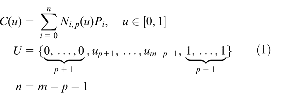
where
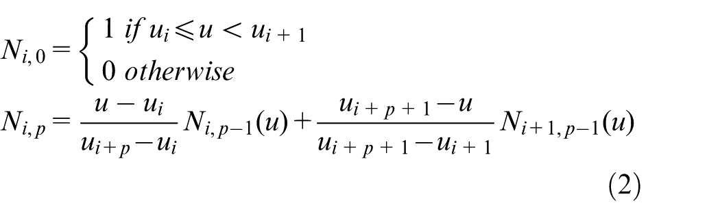
Substituting equation (2) into equation (1), it gets the DeBoor-Cox recursive algorithm 4
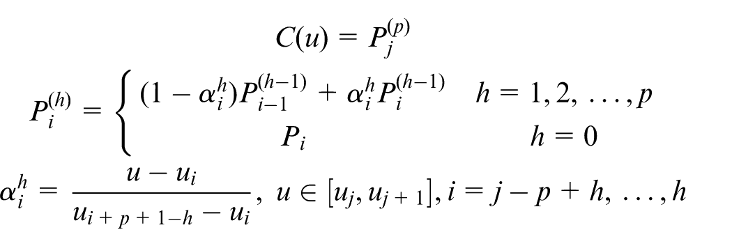
where
Summary of the arithmetic operations for DeBoor-Cox algorithm.
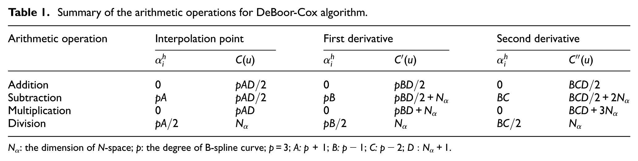
Nα: the dimension of N-space; p: the degree of B-spline curve; p = 3; A: p + 1; B: p − 1; C: p − 2;
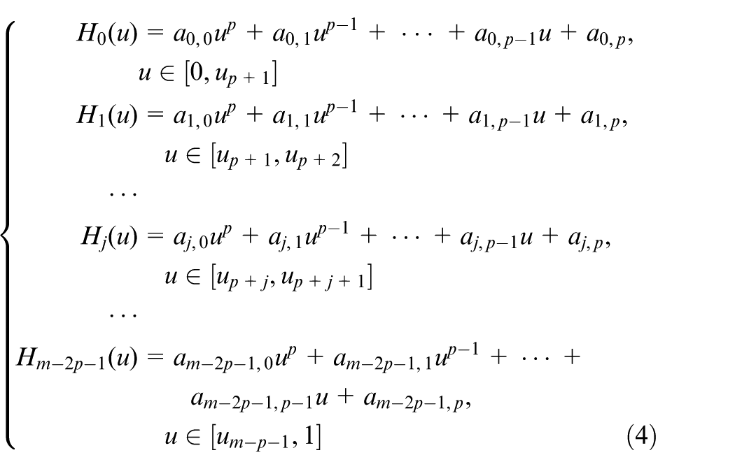
With the DeBoor-Cox algorithm, NC system can implement interpolation process, including curve subdivision, arc-length calculation, and interpolation point generation. However, these operations require to call the DeBoor-Cox algorithm repeatedly, which causes redundant computation. It is noted that the B-spline curve can be converted into piecewise power basis functions as
Then, it becomes much easier to obtain
Summary of the arithmetic operations for the power basis function algorithm.
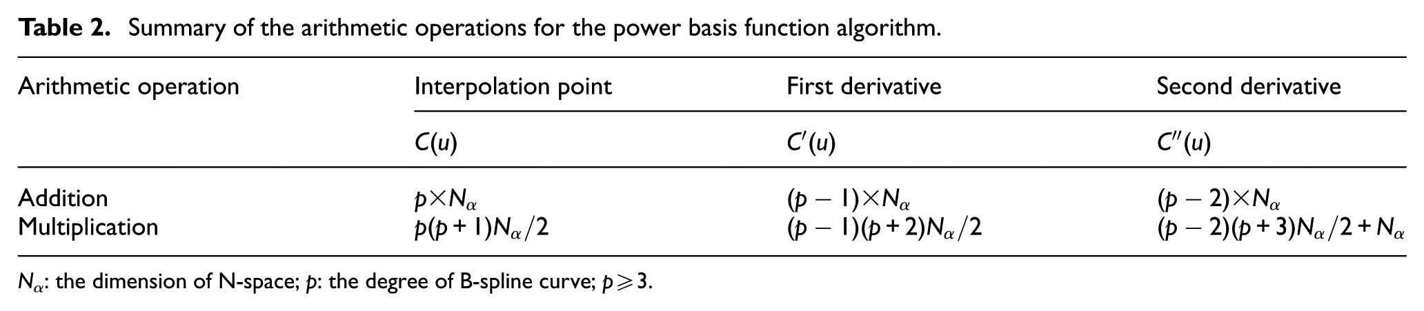
Nα: the dimension of N-space; p: the degree of B-spline curve;
From Tables 1 and 2, the piecewise power basis functions provide less complexity in computation and are easier to be implemented in NC system.
To clearly show the conversion procedure, an example with the cubic B-spline is described in detail below.
Step 1. Convert the B-spline curve
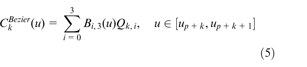
where
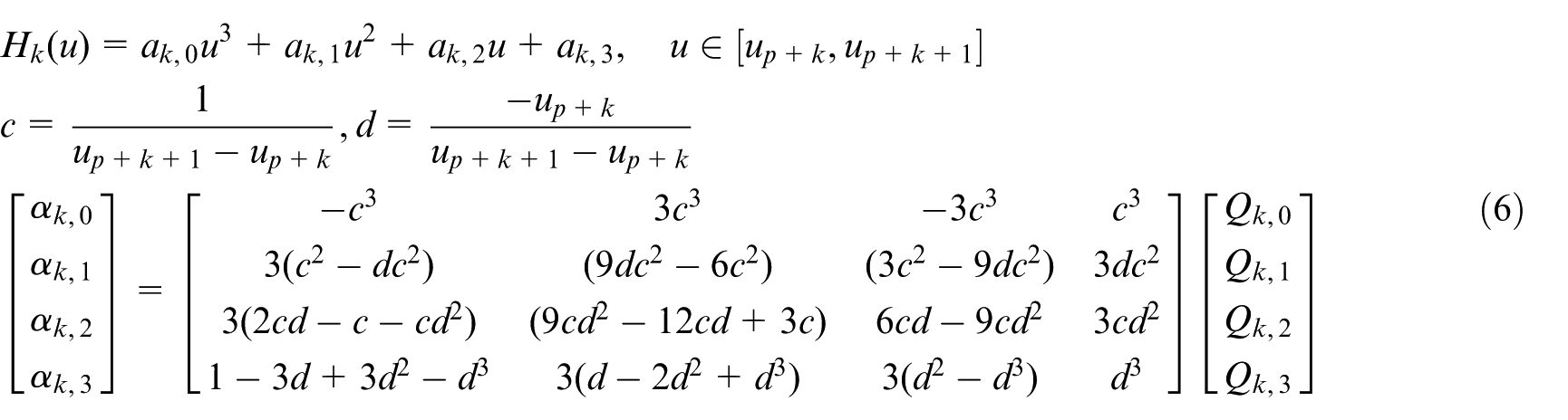
Step 2. Convert each Bézier curve to power basis function by matrix multiplications, for example, the kth power basis function
Step 3. Calculate the first and second derivatives of
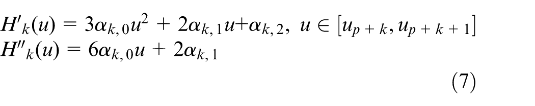
Through above-mentioned steps, a set of power basis functions, whose number is
Summary of the arithmetic operations for curve conversion.
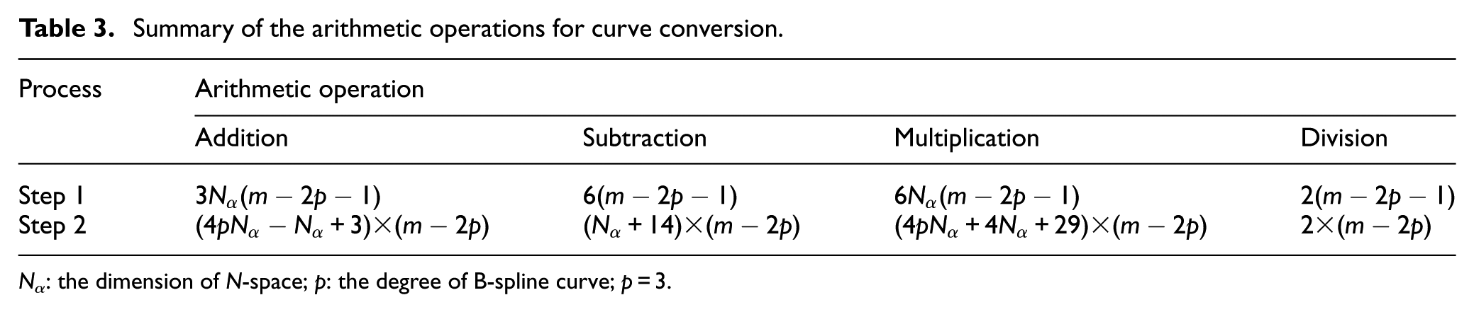
Nα: the dimension of N-space; p: the degree of B-spline curve; p = 3.
Curve subdivision
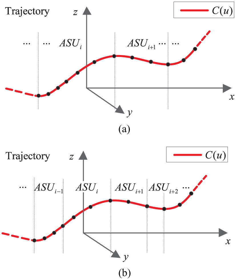
As shown in Figure 1, the traditional interpolation process first executes the pre-interpolation for scanning curvature extrema. Then, the curve subdivision utilizes these extrema to divide the curve and generate ASUs. After that, the arc-length calculation and the ACC/DEC schedule are implemented for each ASU to generate the corresponding velocity profile. In the process, computational load depends on operating the pre-interpolation and calculating arc lengths. 17 With the power basis functions, we can integrate curve subdivision and arc-length calculation to improve the computational efficiency. The process is described in detail as below:
Step 1. Adopt the adaptive Gauss-Legendre quadrature rule to calculate the arc length of
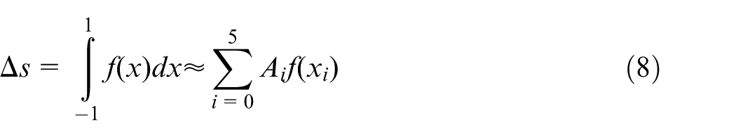
Equation (8) denotes the six-point Gauss-Legendre quadrature rule, and
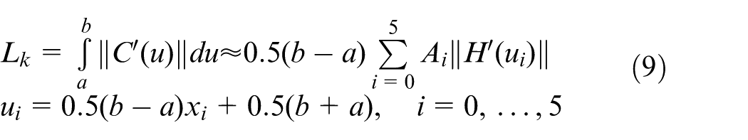
where
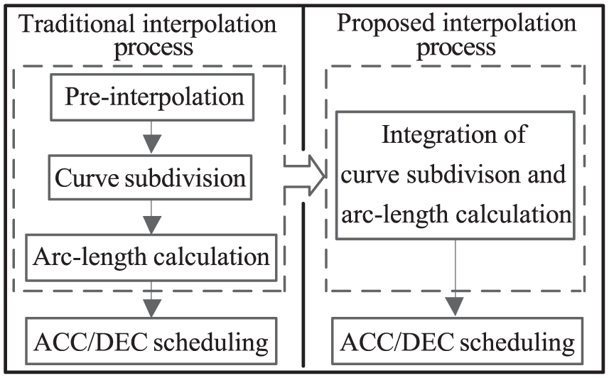
Comparison of the traditional interpolation process and the proposed interpolation process.
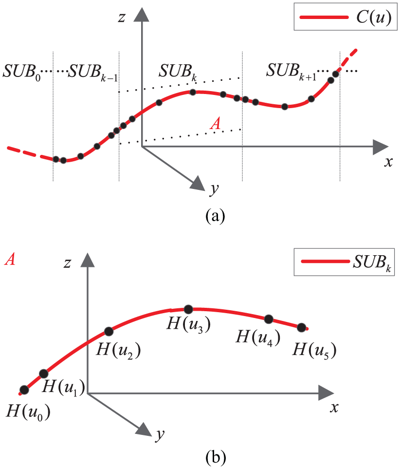
The schematic diagram of SUBs: (a) the distribution of SUBs and (b) the enlarged view of SUBk.
Step 2. Determine curvature extrema and inflection points from the set of generated parameters.
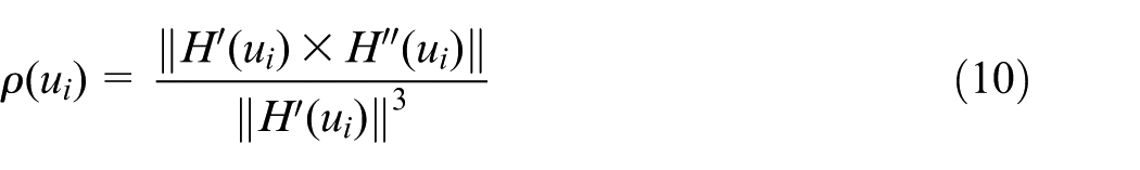
Through scanning the curvatures of these 6n parameters, the curvature extrema of the curve can be roughly determined. Obviously, the tolerance
Define the parameter increment, the arc length increment, and the Gauss node increment as
The parameters at ends of the curve (i.e. 0 and 1).
The parameters
According to this principle, the distribution of interpolation points of selected parameters is much more even, which can be seen in Figure 3(a). Meanwhile, the distribution of that is approximated as follows: 0.1694L0, 0.2113L0, 0.2386L0, 0.2113L0, 0.1694(L0 + L1), 0.2113L1, 0.2386L1, 0.2113L1, …, 0.1694(Ln − 2 + Ln − 1), 0.2113Ln − 1, 0.2386Ln − 1, 0.2113Ln − 1, and 0.1694Ln − 1.
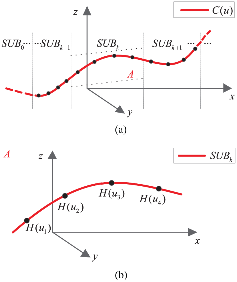
The distribution of the selected points: (a) the selected points on the curve and (b) the selected points on the SUB k .
In this way, NC system only calculates 4n + 2 curvatures in total. Compared with the traditional operation that only curvature extrema are scanned, the proposed operation will scan both curvature extrema and inflection points (as seen in Figure 4). Thus, when ASUs are generated based on these points, only four forms of velocity profiles are needed (i.e. acceleration phase; acceleration and constant velocity phase; deceleration phase; and deceleration and constant phase), which greatly simplifies the ACC/DEC schedule.
Different operations for curve subdivision: (a) the traditional operation and (b) the proposed operation.
Step 3. Calculate the arc length of ASU.
First, determine the subinterval where the endpoint of ASU is located. Then, calculate the relative arc length of ASU in this subinterval by equation (9). After that, accumulate all arc lengths of the previous subintervals. Therefore, the arc length of ASU is estimated with lower computational complexity.
Theoretical computational efficiency comparison
In this section, a cubic B-spline curve is used in the comparison, where the degree of the curve p = 3, the number of control points
Computational efficiency of curve conversion: in section “Conversion from B-spline to piecewise power basis functions,” the arithmetic operations for the curve conversion have been summarized (as seen in Table 3). Thus, the latencies of curve conversion operation can be easily determined, which is equal to 5242. After the curve conversion operation is completed, the B-spline curve is converted to the piecewise power basis functions. With the power basis functions,
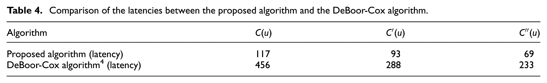
Computational efficiency of curve subdivision: since the arc length is calculated by the adaptive Gauss–Legendre quadrature rule during curve subdivision operation, some parameters of the quadrature formula should be configured before iteration. Here, the initial number of intervals and the maximal number of intervals are 7 and 10, respectively. Meanwhile, assume that the curve is divided into three ASUs after iteration. Accordingly, the latency of the curve subdivison operation based on the power basis functions is 46,515. Under the same parameters, the latency of pre-interpolation algorithm 17 is 130,953. Thus, the latencies of the proposed curve subdivision operation can be reduced by 64.5% compared with that of pre-interpolation algorithm.
Comparison of the latencies between the proposed algorithm and the DeBoor-Cox algorithm.
Experiment validation
Platform construction
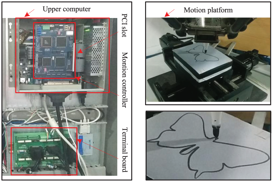
In this section, a motion control platform is set up to verify the proposed algorithm, which consists of an upper computer, a motion controller, and a motion platform:
An upper computer: the computer is configured with Core i5-3470 3.2 GHz CPU, Kingston® DDR3 1600 MHz 8GB memory, and a PC-based NC system. The main parts of NC system, including a smoothing module, a look-ahead ACC/DEC schedule module, an interpolation module, and a timer module, are coded with Visual Studio 2010. Here, the cycle of NC process level is set to 10 ms based on the Win 32 multimedia timer 20 (with 1-ms resolution) and the theoretical interpolation cycle is 1 ms. Thus, NC system can generate 10 interpolation points in each interrupt service routine (ISR).
To generate the interpolation points in real time, all modules are required to collaborate with each other. This collaboration mechanism is defined as the real-time interpolation strategy. Meanwhile, a sliding window is introduced here, which can cover the maximum number of (a) In the first cycle (expressed as (b) In the next cycle, NC system examines whether the tool has reached the window-sliding position (the position where the window 0 and windows 1 overlap). If not reached, only the interpolation module works in this ISR (the
A motion controller: the controller is used to implement the fine interpolation and the closed-loop control, which is based on TMS 320F2812 DSP and Cyclone II FPGA.
A motion platform: the platform consists of an AC servo driver unit and a X-Y platform. The AC servo driver unit consists of two YASKAWA SGDV-2R8A01A Series AC servo drivers and two SGMJV-04ADA21 Series AC servo motors. The movement range of the X-Y platform is 200 mm × 200 mm.
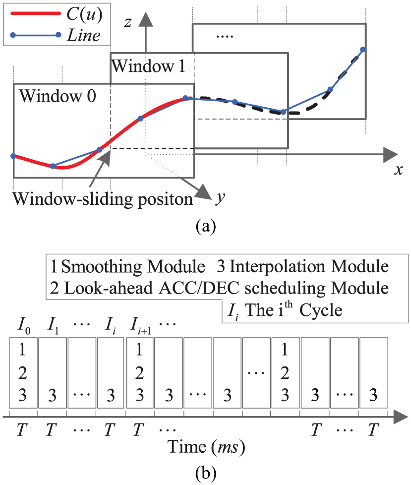
The schematic diagram of real-time interpolation: (a) the machining curve and (b) the program of the NC system.
Interpolation experiment and efficiency analysis
Figure 6 shows a 2D butterfly and a 3D pigeon, which compose of 501 and 270 line segments, respectively. The real-time interpolation for them will be implemented here to verify the effectiveness of the proposed method. In the experiments, the NC system with the proposed method is named as “NC system 1” and the NC system without the proposed curve conversion method is called as “NC system 2.” As seen in Figure 7, after the interpolations for the butterfly pattern, NC system 1 and NC system 2 generate the same number of interpolation points (the number is 34,082). The actual velocity curves are illustrated in Figure 8(a). As shown in the figure, they are completely overlapped. Similarly, for the pigeon pattern, two NC systems have the same generated points (the number is 43,632), the actual velocity curves of which are also completely overlapped as shown in Figure 8(b).
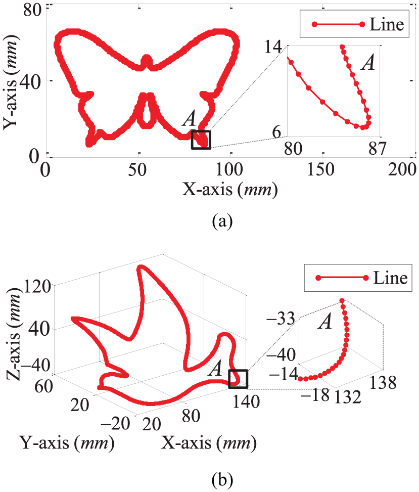
Instances of tool path curves: (a) 2D butterfly and (b) 3D pigeon.
The experiments of real-time interpolation for 2D butterfly pattern.
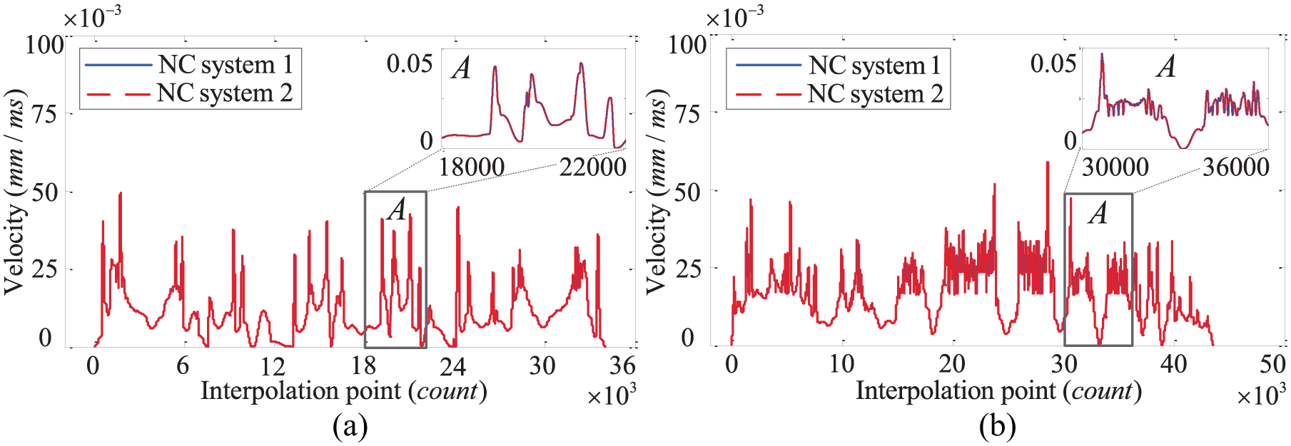
The velocity curves after real-time interpolation: (a) the butterfly pattern and (b) the pigeon pattern.
To exactly record the code execution time in the experiments, two Win 32 API functions, QueryPer
For the butterfly pattern, the execution time of the curve conversion and curve subdivision with NC system 1 is illustrated in Figure 9(a). The execution time of the curve subdivision with NC system 2, which directly utilizes the DeBoor-Cox algorithm,
5
is exhibited in Figure 9(b). Clearly, in Figure 9, (a) and (b) have the same shape but different execution times, especially at the moments when it is required to frequently calculate interpolation points and derivatives. As seen in Figure 9(a), arrow 1 denotes the execution time of curve conversion and curve subdivision in the first cycle. According to the sliding window characteristics,
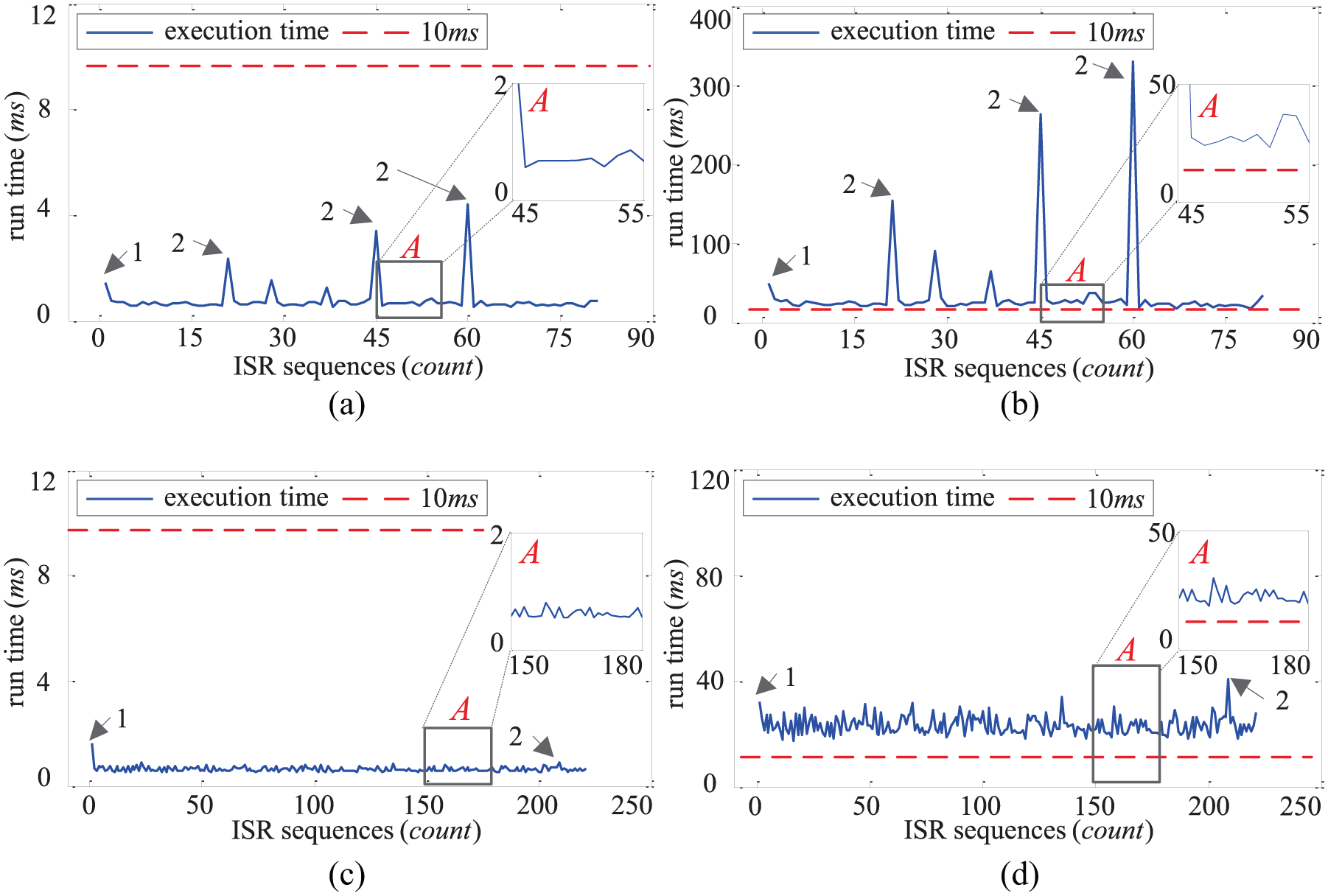
Execution times of curve conversion and curve subdivision with NC system 1 and execution times of curve subdivision with NC system 2: (a) interpolation for butterfly pattern by NC system 1, (b) interpolation for butterfly pattern by NC system 2,(c) interpolation for pigeon pattern by NC system 1, and (d) interpolation for pigeon pattern by NC system 2.
The traditional interpolation process needs to implement the pre-interpolation, and the computation is obviously much more than the proposed process. In this article, we simplify the traditional interpolation process by combing the curve subdivision with arc-length calculations, so the execution time with NC system 1 is less than 10 ms, as shown in Figure 9(a). Here, both the error threshold
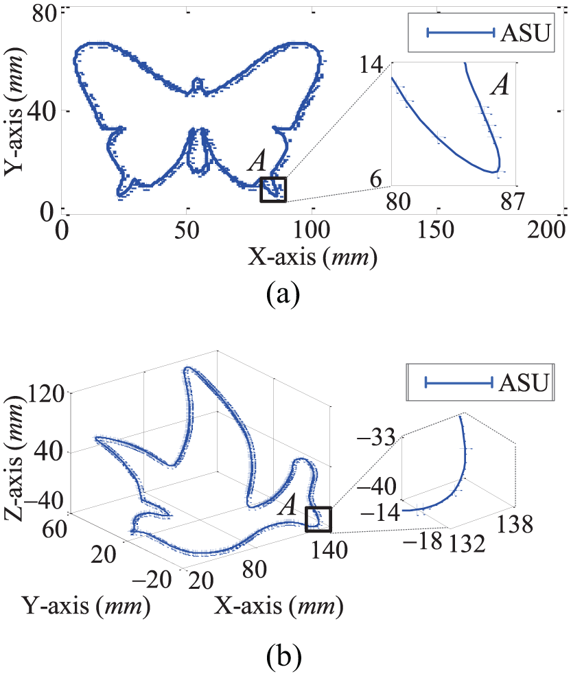
The distribution of the ASUs: (a) on the butterfly pattern and (b) on the pigeon pattern.
A comprehensive evaluation for the proposed method is also given by recording the execution time of each ISR. When real-time interpolations for butterfly pattern is finished, NC system 1 and NC system 2 all generate 3408 ISRs. According to the previous analysis, some execution times of ISRs may exceed the time interval (i.e. 10 ms). In this case, the ISR will not quit until all calculations are completed. Obviously, it will impact the machining quality and efficiency. As shown in Figure 11(a), when NC system 1 is applied, all ISRs are less than the time interval. However, NC system 2 exists the problem that the execution time of some ISRs exceeds the time interval which is 10 ms, as shown in Figure 11(b). From the previous analysis, the execution time with NC system 2 is 10 times higher than that with NC system 1.
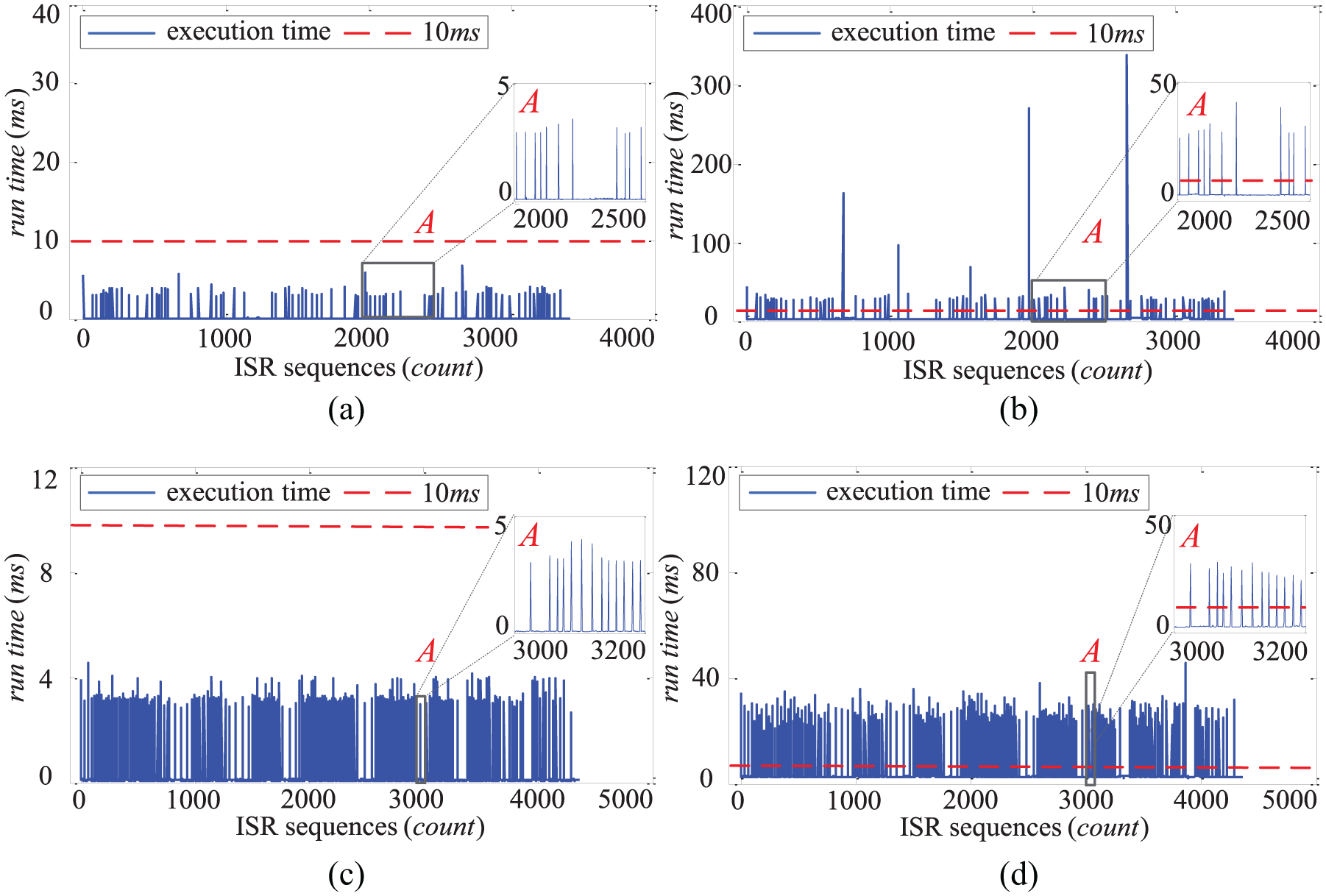
Different execution times of the real-time interpolation: (a) interpolation for butterfly pattern by NC system 1, (b) interpolation for butterfly pattern by NC system 2, (c) interpolation for pigeon pattern by NC system 1, and (d) interpolationfor pigeon pattern by NC system 2.
Similarly, for the pigeon pattern, Figure 9(c) and (d) denotes the execution times of the curve conversion and curve subdivision with NC system 1 and with NC system 2, respectively. Figure 10(b) gives the distribution of the generated ASUs. In addition, the execution times of each ISR with NC system 1 and NC system 2 are illustrated in Figure 11(c) and (d), respectively. From these figures, it can be seen that the efficiency of the NC system can be greatly improved by the proposed method.
Conclusion
This article proposes an algorithm for real-time interpolation based on piecewise power basis functions, which converts the B-spline into power basis functions. Since the interpolation point and the derivative formula can be established explicitly based on the power basis functions, interpolation points and their derivatives can be rapidly computed. Meanwhile, the curve subdivision based on the piecewise power basis functions is implemented, which can further simplify the interpolation process. Thus, the real-time performance for the interpolation can be improved greatly. Theoretical analysis illustrates that the latencies of the proposed curve conversion method and the curve subdivision method can be reduced by 71.1% and by 64.5% compared with the DeBoor-Cox algorithm and the pre-interpolation method. Experiments are carried out with a 2D butterfly and a 3D pigeon, and the results show that the proposed method can greatly improve the computational efficiency.
Footnotes
Declaration of conflicting interests
The author(s) declared no potential conflicts of interest with respect to the research, authorship, and/or publication of this article.
Funding
The author(s) disclosed receipt of the following financial support for the research, authorship, and/or publication of this article: This work was supported, in part, by National Key Basic Research Program of China (Grant No. 2013CB035804), National Science and Technology Major Project (Grant No. 2015ZX04005006), and State Key Lab of Digital Manufacturing Equipment & Technology (Grant No. DMETKF2016002).