Sage Journals: Discover world-class research

Abstract

The positioning error of ball screw feed systems is mainly caused by thermal elongation of the screw shaft in machine tools. In this article, an adaptive on-line compensation method of positioning error for the ball screw shaft is established. In order to explore the thermal–solid mechanism of ball screw feed drive systems, the experiments were carried out. An exponential fitting equation is presented to obtain the temperature relationship between the temperature sensitive point and its center of each heat source based on the finite element method of the feed drive system. Consequently, based on time and position exponential distribution functions, a variable separation model of heat transfer is established. Furthermore, based on the heat transfer model of multiple varying and moving heat sources, an adaptive on-line analytical compensation model of positioning error is presented. Finally, the effect of the adaptive on-line analytical compensation model of positioning error is verified through the experiments. And, this model has self-adaptive ability and robustness. Therefore, this adaptive on-line analytical compensation model based on the heat transfer theory can be applied in real-time compensation of positioning error.

Keywords

Ball screw machine tools varying and moving heat sources adaptive on-line compensation model positioning error

Introduction

It is the thermal expansion of the structural linkages of a ball screw feed drive system that results in inaccuracy in the positioning of the tool.^1–3 Hence, the thermal error is the key factor leading to the dimensional error of machined work-pieces in the machine tool feed system. Thermal errors account for 70% of total errors among various error sources of machine tools in the 1990s, and even today, not much has changed in the industry.^4–9 In order to improve the positioning precision, thermal error compensation is a low cost method.^2,8,9 Thermally induced errors have characteristics of non-linearity and time-dependent nature due to no uniform temperature rise in machine tools. The complex thermal behavior is created by the interaction among the system structure, the thermal expansion coefficient, the heat source location, and the heat source intensity.¹⁰

The accurate and robust modeling of thermal errors is a key step for the implementation of error compensation. Two common methods are used for the compensation of thermal errors. The first one uses empirical modeling to obtain the relationship between the temperature data and the thermal errors. Many researchers proposed a lot of methods, which have been used for modeling and prediction of thermal errors, such as artificial neural networks,^11–16 regression theory,^17–20 gray system theory,²¹ support vector machines,^22,23 fuzzy logic,²⁴ and Bayesian theory.²⁵ However, most of the proposed models assume that the component errors have already been obtained, these errors have to be collected by tedious and time-consuming experiments, actually.

The second method uses numerical analysis to evaluate the thermal error. The numerical method (finite element method (FEM)) and finite difference method (FDM) have been proposed in the thermal error modeling. Mian et al.²⁶ used FEM to build a new off-line thermal error modeling right. Li et al.²⁷ proposed a thermal error model of spindles based on multiple variables for machine tools. Mayr et al.²⁸ calculated the temperature variation using FDM, then calculated thermal errors using FEM. However, it is difficult to establish accurate thermal error models. That is because the boundary conditions of thermal error models are difficultly determined due to the complex structure of machine tools and the varying heat flow resulting in the constantly changing heat flow rate of heat sources and the convention coefficient. Therefore, it is hard to maintain the accuracy and robustness of the compensation model in the actual application.

Besides, many other methods were also proposed to model the thermal errors. Wang et al.²⁹ proposed a new method of real-time compensation of positioning error for computerized numerical controlled (CNC) milling machines based on Newton interpolation method. Wang et al.³⁰ established an interpolation algorithm based on shape functions for error prediction and developed a recursive compensation software. Xiang et al.³¹ established thermal error prediction method for spindles in machine tools based on a hybrid model. Liu et al.³² proposed a modeling method without temperature sensors for half-closed-loop feed drive systems to realize the compensation for thermal errors induced by moving in a constant temperature environment. However, hardly any of the analytical methods of modeling are proposed in these presented models.

In order to solve the above problems, in this article, the FEM integrated with Monte Carlo method is used to capture the multiple varying heat generation rates and obtain the fitting equation on the relationship between the measured temperature of sensitive points and the center temperature of each heat source of the ball screw system in the work. Finally, a new variable separation model of heat transfer is established, and this new model bases on two exponential distribution functions, which are a time function and a position function. The new model makes it possible to obtain the analytic solutions of complicated questions. Furthermore, the proposed adaptive on-line analytical compensation model based on the new variable separation model of multiple varying and moving heat sources is used to predict the temperature distribution and compensate the positioning error of ball screw feed drive systems. By monitoring the temperature sensitive points of the bearing seats and moving-nut flank, this proposed method can realize on-line compensation for the positioning error of ball screw feed drive systems with multiple varying and moving heat sources. This model has self-adaptive ability and robustness.

FEM model integrated with theMonte Carlo method

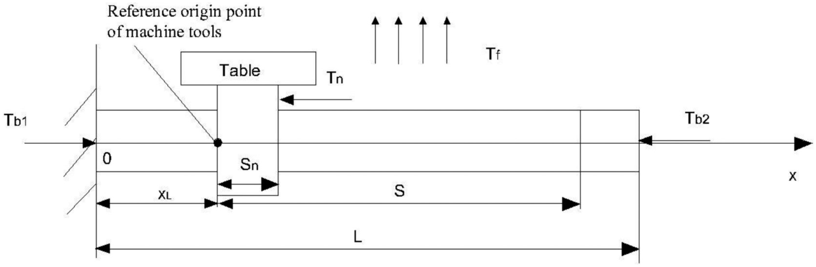
In this study, the FEM integrated with the Monte Carlo method is used to capture multiple varying heat generation rates and explore the solid–thermal mechanism, the temperature distribution, and the thermal error distribution of ball screw feed drive systems. The structure of ball screw feed drive systems is shown in Figure 1 and consists of supporting bearing 1, supporting bearing 2, and moving-nut.

Figure 1.

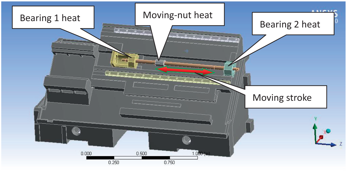
Schematic of heat source distribution and stroke range.

A CONTA174 contacting element is used to simulate the contact areas and a SOLID87 solid element is chosen to calculate the temperature field of the ball screw system. There are totally 54,792 solid elements and 8496 contact elements.

In this work, the temperature field is analyzed based on the following assumptions:^7,8

The friction heat generated by a ball screw pair has uniform distribution.

The screw rod is simplified into a cylinder.

The bearings are hollow cylinders.

The moving-nut is a hollow cylinder.

The radiation term can be neglected for smaller temperature increases.

Convective heat coefficients are always constant during motion at the same feed rate.

Heat transfer coefficient

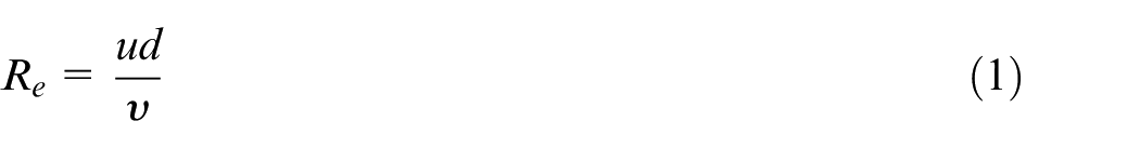
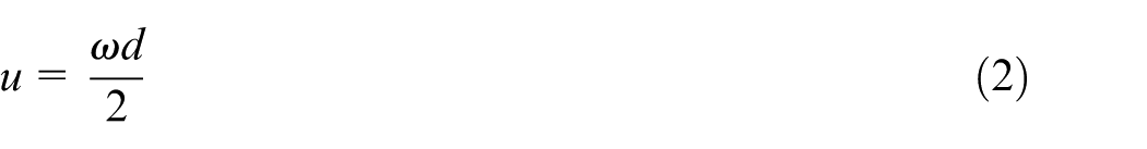
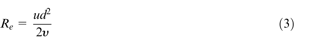
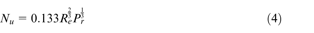
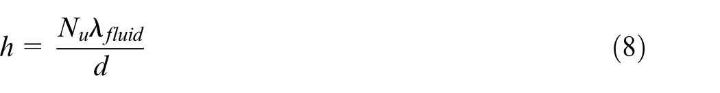
The forced convection results in heat loss. The heat transfer coefficient for convection of the screw shaft was calculated based on the following steps. Reynolds number of the screw shaft can be written as

R_{e} = \frac{ud}{υ}

(1)

where $u$ is the velocity of the screw shaft. It is defined as

u = \frac{ω d}{2}

(2)

where $ω$ is the angular velocity of the screw shaft, and $d$ is the diameter of the screw shaft. The expression for Reynolds number can be rewritten as

R_{e} = \frac{u d^{2}}{2 υ}

(3)

where $R_{e}$ is the Reynolds number, and $υ$ is the kinematic viscosity of fluid. The Nusselt number is determined by

N_{u} = 0.133 R_{e}^{\frac{2}{3}} P_{r}^{\frac{1}{3}}

(4)

Equation (4) is applicable to

R_{e} < 4.3 \times 10^{5}

(5)

0.7 < P_{r} < 670

(6)

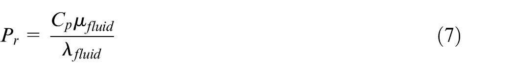
The Prandtl number is expressed as

P_{r} = \frac{C_{p} μ_{fluid}}{λ_{fluid}}

(7)

where $C_{p}$ denotes the specific heat capacitance of the air, $μ_{fluid}$ is the dynamic viscosity, and $λ_{fluid}$ is the thermal conductivity of the air. $P_{r}$ is 0.707 for air. The heat transfer coefficient $h$ of the screw shaft is written as

h = \frac{N_{u} λ_{fluid}}{d}

(8)

The feed rate of the bed saddle of ball screw feed drive systems is relatively low. Hence, the effect of the forced convection was ignored. The convection coefficient of 12 W/m² K was assigned to the bed saddle, bearing seats, and housing surfaces.³³

Implementation of the FEM model

The ANSYS software package integrated with the Monte Carlo method was developed to study thermal–solid mechanism of the ball screw feed drive system. The diagram of the FEM/Monte Carlo method is shown in Figure 2. In this study, the FEM/Monte Carlo method is executed based on the following steps:

Initial guesses for the three heat flows of supporting bearing 1, supporting bearing 2, and moving-nut are applied in the FEM simulation to obtain the temperature distribution of the ball screw system. If the numerical results on the key points obtained by FEM do not agree with the measured results, the estimated range values of the three heat flows were assigned to the boundary values of the Monte Carlo method and then the Monte Carlo method generates multiple sets of intermediate values according to the given sampling times p. Each set of intermediate values was used as the boundary conditions of FEM, and the resulting distribution can be obtained. Once the process is finished, the numerical and experimental results that are in good agreement can be adopted. In addition, the heat convection coefficient is obtained from the heat transfer equation (equation (8)).

By the FEM model of the feed drive system, the friction heat flow rates of the bearing 1, bearing 2, and moving-nut can be obtained automatically using the FEM/Monte Carlo method. The friction power allocation in heat sources of the feed drive system is found.

Using the adaptive thermal–solid model based on the FEM/Monte Carlo method, the temperature distribution between the measured point and the center of each heat source can be obtained and the thermal deformation of various elements of the ball screw feed drive system can be obtained. The method is resolved automatically using the Monte Carlo method. Therefore, the efficiency of the method is high, and it is used to resolve multiple varying parameter model for the complex system.

Figure 2.

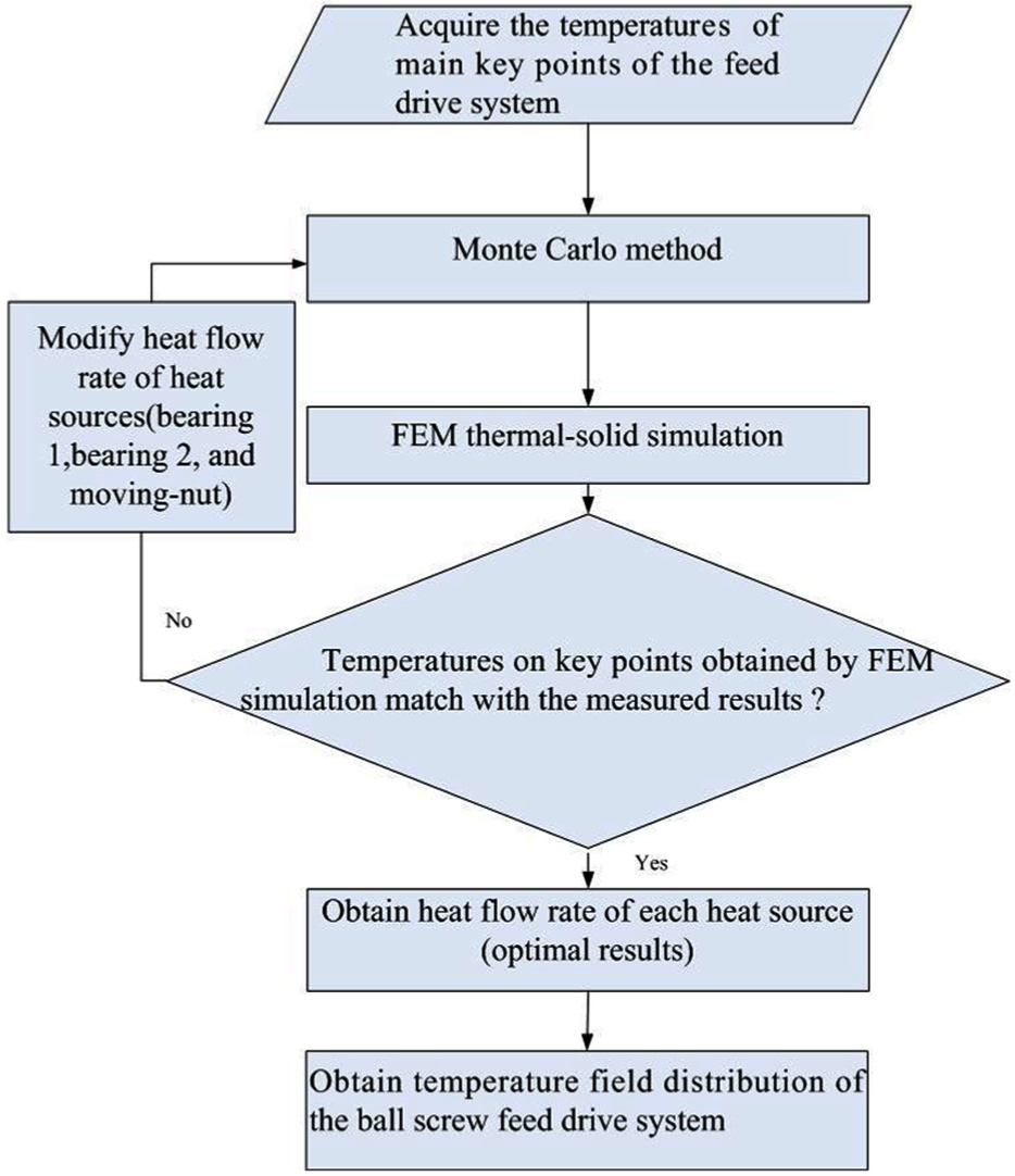
Diagram of FEM/Monte Carlo method of ball screw feed drive systems.

Temperature distribution rule between the measured point and the center of heat sources

The center temperature of each heat source is important for exploring thermal characteristics. However, the center temperature of each heat source is difficult to measure because the sensor could not be put into the prescribed position.

Li et al.⁸ explored the thermal characteristics of the ball screw under the different feed rates by experiments. The measured results prove that the temperature rise of the ball screw always shows a stable exponential rise under different feed rates.

In this study, the relationship between the measured point temperature and center temperature of each heat source is explored using the FEM model.

The temperatures of the bearing 1, bearing 2, and moving-nut always show a stable exponential rise under different feed rates. In addition, the temperature difference between the measured point and the center of each heat source in the bearing 1, bearing 2, and moving-nut always shows a stable exponential rise under different feed rates. The stable temperature rise increases linearly as the feed rate increases. In this work, the experimental results are similar to Li et al.⁸

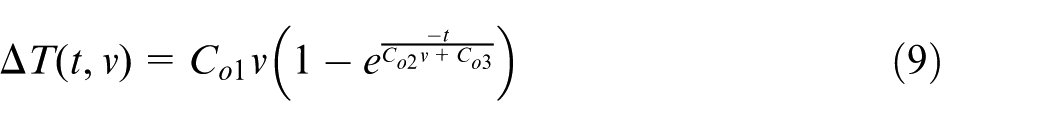
Therefore, the equation for the temperature difference between the measured point and the center of each heat source can be fitted by an exponential function. The fitting equation for the temperature difference $Δ T (t, v)$ is written as

Δ T (t, v) = C_{o 1} v (1 - e^{\frac{- t}{C_{o 2} v + C_{o 3}}})

(9)

where $v$ is the feed rate of the carriage, $t$ is the working time, and $C_{o 1}$ , $C_{o 2}$ , and $C_{o 3}$ are the constants obtained by exponential fit.

The real-time temperature measured from a measured point on the surface is collected by thermocouples. The center temperature for the heat source is the sum of the fitting equation of temperature difference and the real-time temperature measured from a sensitive point on the surface

T_{c} = T_{m} + Δ T (t, v)

(10)

where $T_{c}$ is the center temperature of the heat source, and $T_{m}$ is the real-time temperature of a point measured on the surface.

Using thermocouple readings as inputs, this equation can be used to predict the temperature of the center of the heat source in real time. The equations for the bearing 1, bearing 2, and moving-nut are simultaneously obtained by this method.

This method establishes a foundation to reveal the thermal–solid coupling mechanism of the ball screw feed drive system in real time.

Adaptive analytical model of the positioning error

Equation of heat conduction of multiple varying and moving heat sources

The influences on elongation of the screw shaft due to the friction heat of the bearings and moving-nut were taken into account. The machining accuracy of machine tools was mainly affected by the axial thermal elongation of the screw shaft. Therefore, the radial thermal deformation of the screw shaft was not taken into account.

The left end of the screw shaft was fastened, and the right end of it was free, as shown in Figure 3.

Figure 3.

Heat transfer of ball screw systems.

The equation of heat conduction of the ball screw is written as

{\begin{matrix} \frac{\partial^{2} T (x, t)}{\partial x^{2}} = \frac{ρ c}{k} \frac{\partial T (x, t)}{\partial t} + \frac{4 h}{kd} (T (x, t) - T_{f} (t)) \\ T (x, 0) = T_{f} (0) \\ T (0, t) = T_{b 1} (t_{j}) \\ T (L, t) = T_{b 2} (t_{j}) \\ T (x, t) = T_{n} (x_{i}, t_{j}) \\ T_{f} (x, t) = T_{f} (t_{j}) \end{matrix} x \in [0, S]

(11)

where $T (x, t)$ denotes the temperature of the ball screw and is a function of time $t$ and the distance $x$ , $k$ denotes the thermal conductivity, $ρ$ denotes the material density of the ball screw, c denotes the specific heat capacity, $T_{f} (t)$ denotes the temperature of the ambient air, $T_{b 1} (t_{j})$ denotes the center temperature of bearing 1, $T_{b 2} (t_{j})$ denotes the center temperature of bearing 2, $T_{n} (t_{j})$ denotes the center temperature of moving-nut, $S$ denotes the stroke of moving-nut, and $x_{L}$ denotes the non-working section on the left of the screw shaft.

Using the variable separation method, the temperature of the ball screw $T (x, t)$ is written as

T (x, t) = T_{t} (t) \cdot T_{p} (x)

(12)

where the time function $T_{t} (t)$ is written as

T_{t} (t) = A (1 - e^{- \frac{t}{B}})

(13)

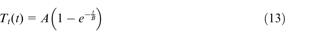
The position function $T_{p} (x)$ is written as

T_{p} (x) = C e^{- \frac{x}{D}}

(14)

where A, B, C, and D are the constants. Therefore, the temperature of the ball screw $T (x, t)$ is rewritten as

T (x, t) = A (1 - e^{- \frac{t}{B}}) \cdot C e^{- \frac{x}{D}}

(15)

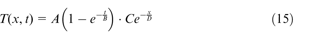
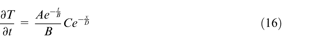
The first-order derivative of the temperature versus time is written as

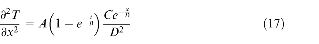
\frac{\partial T}{\partial t} = \frac{A e^{- \frac{t}{B}}}{B} C e^{- \frac{x}{D}}

(16)

The second-order derivative of the temperature versus position of the ball screw is written as

\frac{\partial^{2} T}{\partial x^{2}} = A (1 - e^{- \frac{t}{B}}) \frac{C e^{- \frac{x}{D}}}{D^{2}}

(17)

Set $P = ρ c / k$ and $Q = 4 h / kd$ . Then, equation (11) is rewritten as

\frac{\partial^{2} T}{\partial x^{2}} - P \frac{\partial T}{\partial t} - Q (T - T_{f}) = 0

(18)

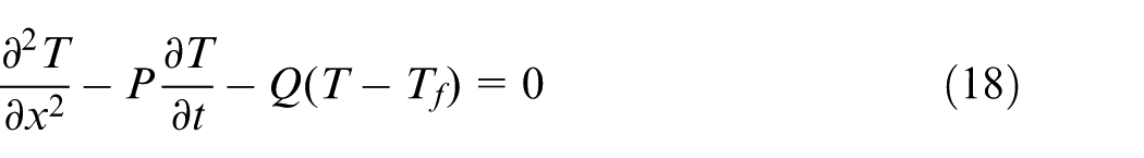
Substituting equations (12), (16), and (17) into equation (18) yields

A (1 - e^{- \frac{t}{B}}) \frac{C e^{- \frac{x}{D}}}{D^{2}} - P \frac{A e^{- \frac{t}{B}}}{B} C e^{- \frac{x}{D}} - Q (A (1 - e^{- \frac{t}{B}}) \cdot C e^{- \frac{x}{D}} - T_{f}) = 0

(19)

Substituting equation (15) into equation (19), equation (19) is rewritten as

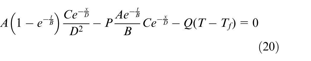
A (1 - e^{- \frac{t}{B}}) \frac{C e^{- \frac{x}{D}}}{D^{2}} - P \frac{A e^{- \frac{t}{B}}}{B} C e^{- \frac{x}{D}} - Q (T - T_{f}) = 0

(20)

The analytical solution of equation (20) is

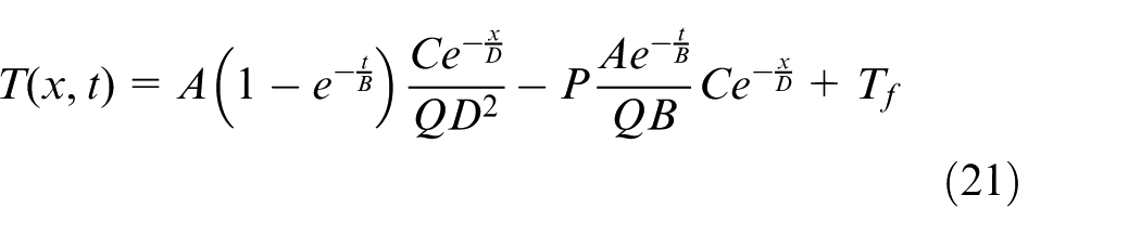
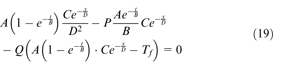
T (x, t) = A (1 - e^{- \frac{t}{B}}) \frac{C e^{- \frac{x}{D}}}{Q D^{2}} - P \frac{A e^{- \frac{t}{B}}}{QB} C e^{- \frac{x}{D}} + T_{f}

(21)

Equation (21) is adaptive to not only an unilateral heat transfer but also a bilateral heat transfer. For bearing 1, the heat transfer equation is written as

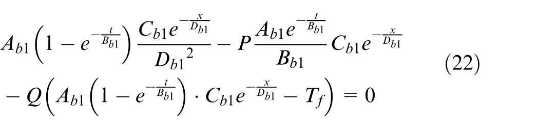
A_{b 1} (1 - e^{- \frac{t}{B_{b 1}}}) \frac{C_{b 1} e^{- \frac{x}{D_{b 1}}}}{{D_{b 1}}^{2}} - P \frac{A_{b 1} e^{- \frac{t}{B_{b 1}}}}{B_{b 1}} C_{b 1} e^{- \frac{x}{D_{b 1}}} - Q (A_{b 1} (1 - e^{- \frac{t}{B_{b 1}}}) \cdot C_{b 1} e^{- \frac{x}{D_{b 1}}} - T_{f}) = 0

(22)

Substituting equation (15) into equation (22), equation (22) can be rewritten as

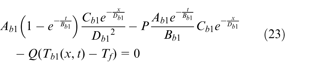
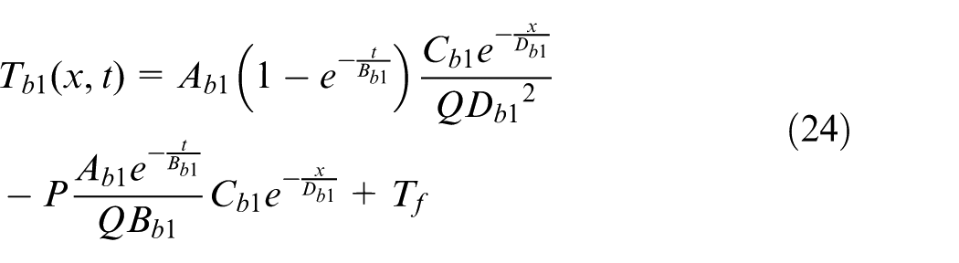
A_{b 1} (1 - e^{- \frac{t}{B_{b 1}}}) \frac{C_{b 1} e^{- \frac{x}{D_{b 1}}}}{{D_{b 1}}^{2}} - P \frac{A_{b 1} e^{- \frac{t}{B_{b 1}}}}{B_{b 1}} C_{b 1} e^{- \frac{x}{D_{b 1}}} - Q (T_{b 1} (x, t) - T_{f}) = 0

(23)

The analytical solution of equation (23) is

T_{b 1} (x, t) = A_{b 1} (1 - e^{- \frac{t}{B_{b 1}}}) \frac{C_{b 1} e^{- \frac{x}{D_{b 1}}}}{Q {D_{b 1}}^{2}} - P \frac{A_{b 1} e^{- \frac{t}{B_{b 1}}}}{Q B_{b 1}} C_{b 1} e^{- \frac{x}{D_{b 1}}} + T_{f}

(24)

For bearing 2, the heat transfer equation is written as

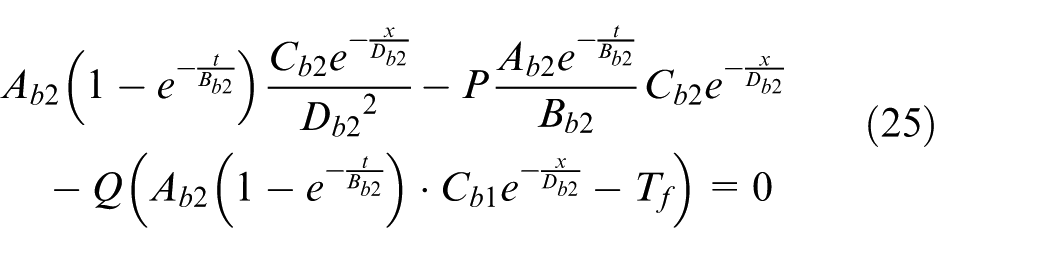
A_{b 2} (1 - e^{- \frac{t}{B_{b 2}}}) \frac{C_{b 2} e^{- \frac{x}{D_{b 2}}}}{{D_{b 2}}^{2}} - P \frac{A_{b 2} e^{- \frac{t}{B_{b 2}}}}{B_{b 2}} C_{b 2} e^{- \frac{x}{D_{b 2}}} - Q (A_{b 2} (1 - e^{- \frac{t}{B_{b 2}}}) \cdot C_{b 1} e^{- \frac{x}{D_{b 2}}} - T_{f}) = 0

(25)

Substituting equation (15) into equation (25), equation (25) can be rewritten as

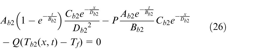
A_{b 2} (1 - e^{- \frac{t}{B_{b 2}}}) \frac{C_{b 2} e^{- \frac{x}{D_{b 2}}}}{{D_{b 2}}^{2}} - P \frac{A_{b 2} e^{- \frac{t}{B_{b 2}}}}{B_{b 2}} C_{b 2} e^{- \frac{x}{D_{b 2}}} - Q (T_{b 2} (x, t) - T_{f}) = 0

(26)

The analytical solution of equation (25) is

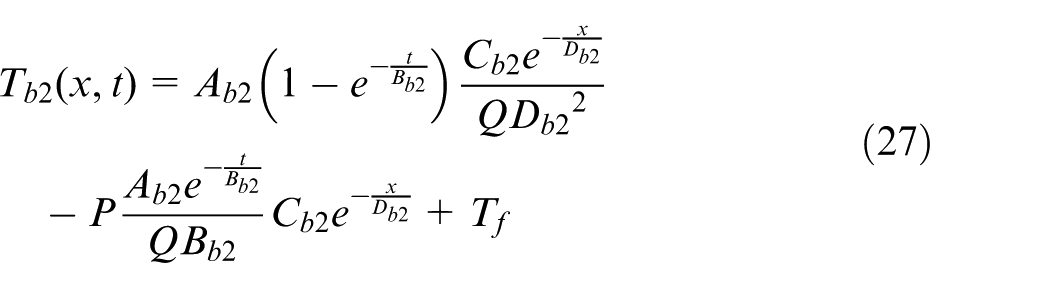
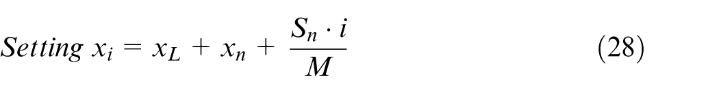
T_{b 2} (x, t) = A_{b 2} (1 - e^{- \frac{t}{B_{b 2}}}) \frac{C_{b 2} e^{- \frac{x}{D_{b 2}}}}{Q {D_{b 2}}^{2}} - P \frac{A_{b 2} e^{- \frac{t}{B_{b 2}}}}{Q B_{b 2}} C_{b 2} e^{- \frac{x}{D_{b 2}}} + T_{f}

(27)

For the moving-nut, the heat source is treated as the superposition of M heat sources, which are continuous distribution within the stroke and along the shaft. The ith heat source is located in $x_{i}$ position

Setting x_{i} = x_{L} + x_{n} + \frac{S_{n} \cdot i}{M}

(28)

where $S_{n}$ is the length of the moving-nut, and $x_{n}$ is the real-time position of moving-nut collected by FANUC Open CNC API Specifications (FOCAS). The heat transfer equation of the ith heat source of moving-nut is written as

A_{n} (1 - e^{- \frac{t}{B_{n}}}) \frac{C_{n} e^{- \frac{| x - x_{i} |}{D_{n}}}}{{D_{n}}^{2}} - P \frac{A_{n} e^{- \frac{t}{B_{n}}}}{B_{n}} C_{n} e^{- \frac{| x - x_{i} |}{D_{n}}} - Q (A_{n} (1 - e^{- \frac{t}{B_{n}}}) \cdot C_{n} e^{- \frac{| x - x_{i} |}{D_{n}}} - T_{f}) = 0

(29)

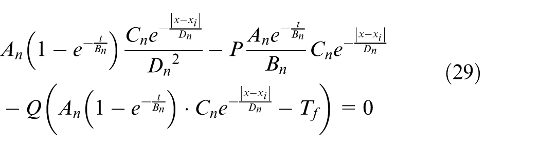
Substituting equation (15) into equation (29), equation (29) can be rewritten as

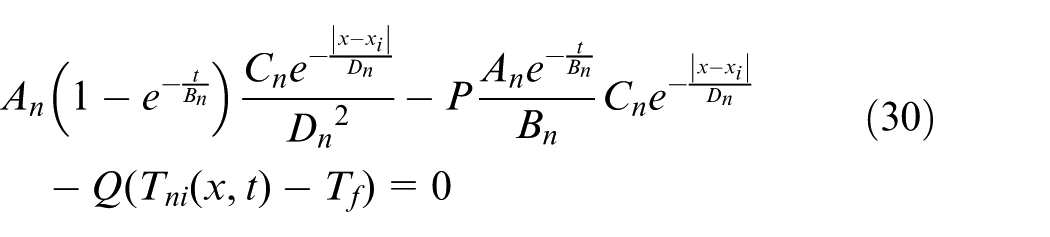
A_{n} (1 - e^{- \frac{t}{B_{n}}}) \frac{C_{n} e^{- \frac{| x - x_{i} |}{D_{n}}}}{{D_{n}}^{2}} - P \frac{A_{n} e^{- \frac{t}{B_{n}}}}{B_{n}} C_{n} e^{- \frac{| x - x_{i} |}{D_{n}}} - Q (T_{n i} (x, t) - T_{f}) = 0

(30)

The analytical solution of equation (30) is

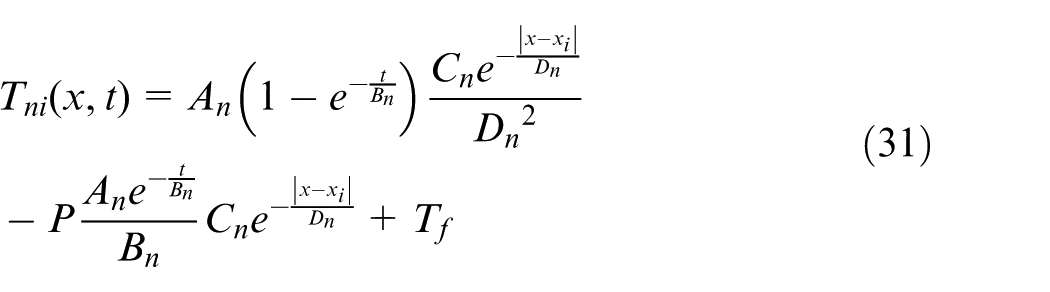
T_{n i} (x, t) = A_{n} (1 - e^{- \frac{t}{B_{n}}}) \frac{C_{n} e^{- \frac{| x - x_{i} |}{D_{n}}}}{{D_{n}}^{2}} - P \frac{A_{n} e^{- \frac{t}{B_{n}}}}{B_{n}} C_{n} e^{- \frac{| x - x_{i} |}{D_{n}}} + T_{f}

(31)

According to temperature superposition method, the temperature rise of the screw shaft is obtained as

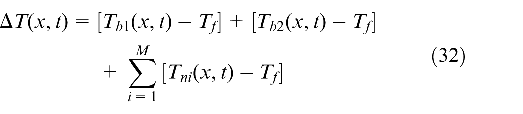
Δ T (x, t) = [T_{b 1} (x, t) - T_{f}] + [T_{b 2} (x, t) - T_{f}] + \sum_{i = 1}^{M} [T_{n i} (x, t) - T_{f}]

(32)

In equation (32), there are the 12 unknown parameters, namely, $A_{b 1}$ , $A_{b 2}$ , $A_{n}$ , $B_{b 1}$ , $B_{b 2}$ , $B_{n}$ , $C_{b 1}$ , $C_{b 2}$ , $C_{n}$ , $D_{b 1}$ , $D_{b 2}$ , and $D_{n}$ . The 12 unknown parameters are obtained by on-line identification. The 12 set of values collected continuously by thermocouples are used for equation (32) in order to identify the 12 unknown parameters when needed. Therefore, when the 12 unknown parameters are obtained, the temperature rise distribution of the ball screw is determined by equation (32) under the working condition.

The real-time temperature measured from a sensitive point on the surface is collected by thermocouples. The center temperature equation for the heat source is the sum of the fitting equation of temperature rise and the real-time temperature measured from a measured point on the surface. The temperature rise equation for the center of bearing 1 is written as

T_{b 1 c} = T_{b 1 m} + Δ T_{b 1} (t, v)

(33)

The temperature rise equation for the center of bearing 2 is written as

T_{b 2 c} = T_{b 2 m} + Δ T_{b 2} (t, v)

(34)

The temperature rise equation for the center of moving-nut is written as

T_{nc} = T_{nm} + Δ T_{n} (t, v)

(35)

Thermal error of the screw shaft

The temperature rise of key components used in ball screw feed drive systems is caused by friction heat of kinematic pairs. Furthermore, the temperature rise results in the thermal elongation of the screw shaft. This thermal elongation causes the thermal error of ball screw feed drive systems.

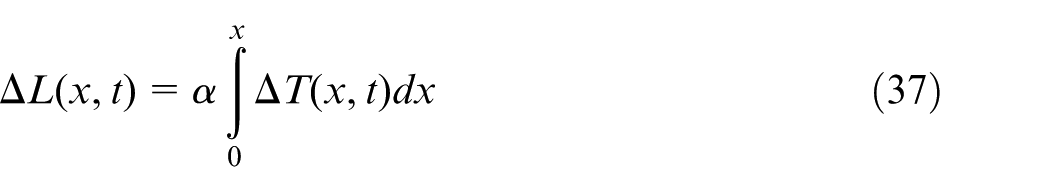
The axial thermal elongation value of a cylinder can be written as

Δ L = L \cdot α \cdot Δ T

(36)

where $L$ denotes the length of the cylinder, $α$ denotes the coefficient of linear thermal expansion, $Δ T$ denotes the temperature rise of the cylinder, and $Δ L$ denotes the axial thermal elongation value.

Hence, the axial thermal elongation value of the screw shaft can be expressed as

Δ L (x, t) = α \int_{0}^{x} Δ T (x, t) dx

(37)

where $Δ L (x, t)$ indicates the thermal elongation value at time of t, and $Δ T (x, t)$ denotes the temperature variation of the screw shaft.

Positioning error of the screw shaft

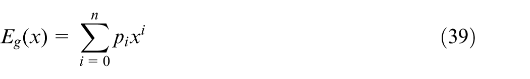
The positioning error of ball screw feed drive systems consists of initial geometric error and thermal error.⁸

The positioning error of the screw shaft in ball screw feed drive systems can be expressed as

E (x, t) = Δ L (x, t) + E_{g} (x)

(38)

where $E (x, t)$ denotes the total positioning error of the screw shaft, and $E_{g} (x)$ denotes the initial geometric error of the screw shaft. The initial geometric error $E_{g} (x)$ is expressed as

E_{g} (x) = \sum_{i = 0}^{n} p_{i} x^{i}

(39)

where $p_{i}$ is the coefficient of the polynomials.

Experimental details

Experimental setup

To explore the thermal–solid coupling mechanism of ball screw feed drive systems in machine tools, experiments were conducted on the z-axis of a CNC lathe with FANUC Series 0i Mate-TD under different feed rates. The experimental setup used for the ball screw shaft system monitoring is shown in Figure 4.

Figure 4.

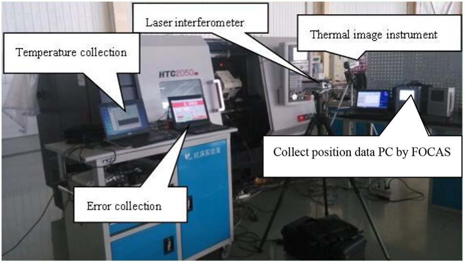
Experimental setup used for the ball screw shaft system monitoring.

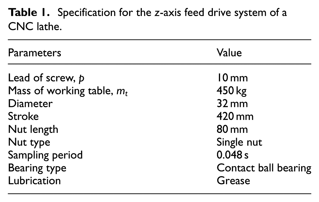
Experimental studies were performed on the CNC lathe. The experimental setup was composed of an infrared thermal imaging instrument, a laser interferometer, and a temperature collection instrument with four thermocouples. The fundamental specifications for the ball screw feed drive system used in the CNC lathe are given in Table 1. A PC with the FOCAS application developed by Visual C++ was used to collect the real-time position of the moving-nut.

Table 1.

Specification for the z-axis feed drive system of a CNC lathe.

Parameters	Value
Lead of screw, $p$	10 mm
Mass of working table, $m_{t}$	450 kg
Diameter	32 mm
Stroke	420 mm
Nut length	80 mm
Nut type	Single nut
Sampling period	0.048 s
Bearing type	Contact ball bearing
Lubrication	Grease

Testing procedure

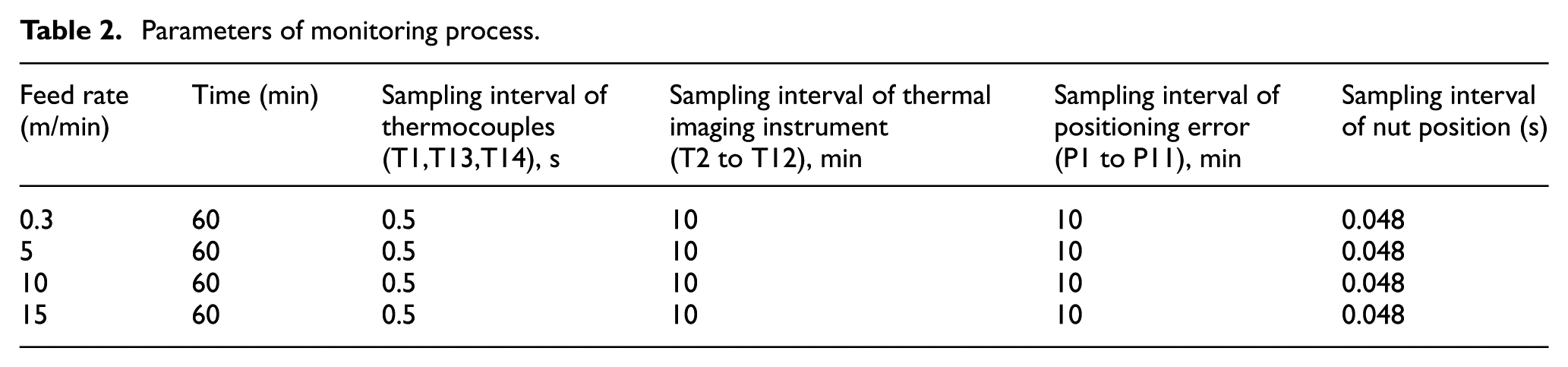
The z-axis feed drive of the CNC lathe was tested using a 0 r/min spindle speed and no load. To obtain the temperature rise and thermal deformation under long-term movement of the table, experiments were performed using the arrangement shown in Figure 5. The parameters of monitoring process are shown in Table 2. Temperatures were measured at the 14 points shown in Figure 5(a). The first and second thermocouples (numbers 1 and 13, respectively) were located on the surfaces of bearing seat 1 and bearing seat 2 with their magnetic bases. The third thermocouple (number 14) was located on the flank surface of the nut. The fourth thermocouple was located on the housing (ambient temperature). The temperature of 11 key points (numbers 2–12) on the screw shaft (shown in Figure 5(a)) is evenly taken. The 11 key points were located on the screw shaft every 42 mm from the reference origin point of the machine up to 420 mm. Movement of the nut along the screw shaft occurs repeatedly between points 2 and 12. Hence, the ball screw system was heated by the movement of the nut along the screw shaft. In order to measure the temperature of the screw shaft, an infrared thermal imaging instrument was used. The temperatures of the key points were measured simultaneously in sampling intervals of 10 min for 0.3, 5, 10, and 15 m/min feed rates.

Figure 5.

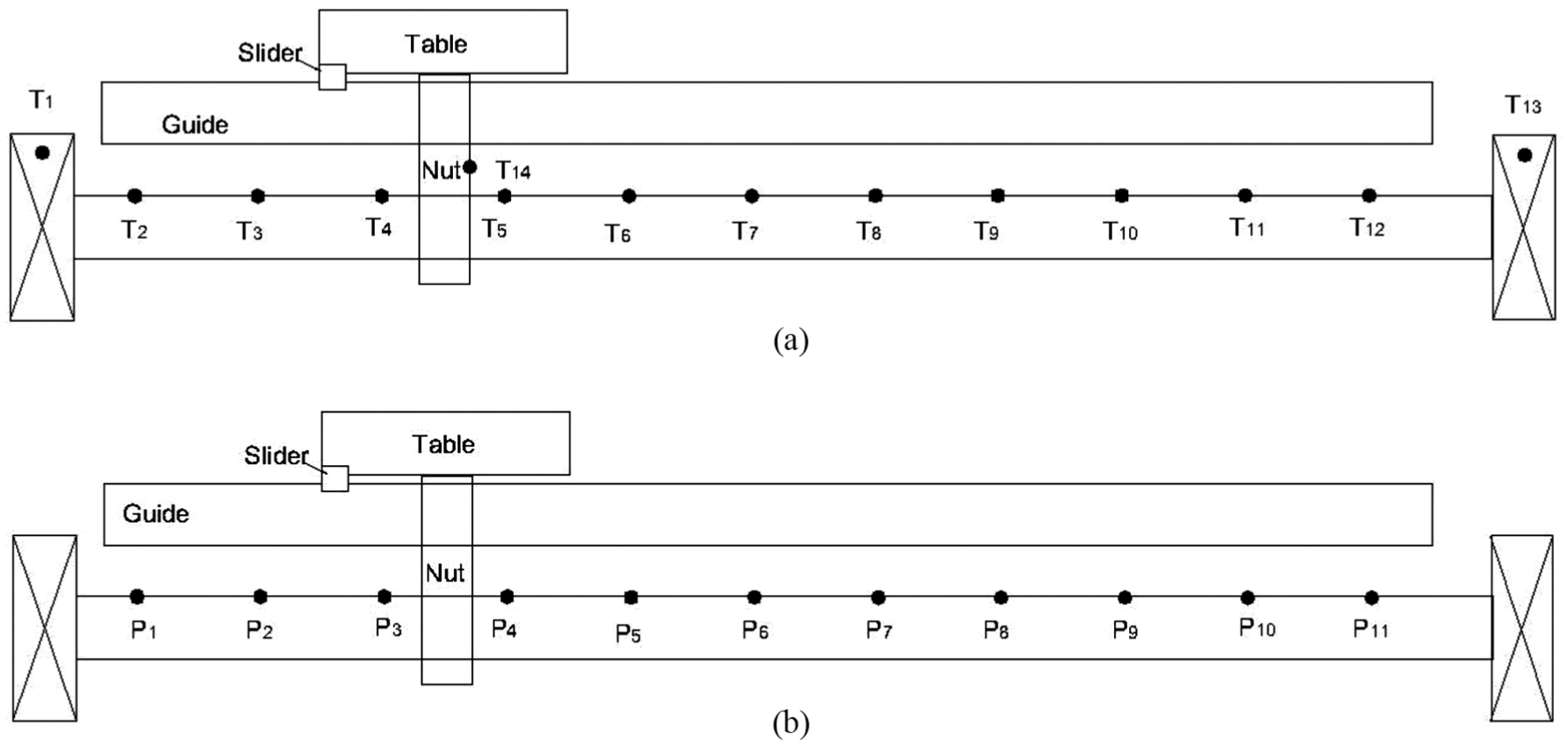
Locations of measuring points for (a) temperatures and (b) thermal errors.

Table 2.

Parameters of monitoring process.

Feed rate (m/min)	Time (min)	Sampling interval of thermocouples (T1,T13,T14), s	Sampling interval of thermal imaging instrument (T2 to T12), min	Sampling interval of positioning error (P1 to P11), min	Sampling interval of nut position (s)
0.3	60	0.5	10	10	0.048
5	60	0.5	10	10	0.048
10	60	0.5	10	10	0.048
15	60	0.5	10	10	0.048

To measure the positioning error of the z-axis feed drive, a laser interferometer was used to obtain the positioning error of the screw shaft. The positioning error of 11 key points (numbers 1–11) on the screw shaft (as shown in Figure 5(b)) is evenly taken, and the 11 key points are located every 42 mm along the entire 420 mm stroke range.

In order to measure the position of the moving-nut, a computer with Visual C++ developing FOCAS application was used to collect the position data of the moving-nut in sampling intervals of 0.048 s.

In this work, the reference origin point of the ball screw feed drive system was designated to be the starting point. Initially, the machine tool was turned on, and the initial geometric error of the screw shaft was collected at room temperature. Subsequently, the ball screw feed drive system was heated by the movement of the nut along the screw shaft with the given feed rate. Moreover, the temperatures of the bearings, moving-nut, and ambient air were taken using thermocouples at an interval of 0.048 s. In addition, the temperatures of the screw shaft were taken using the thermal imaging instrument at an interval of 10 min. The positioning error was collected simultaneously after the ball screw feed drive system had been heated for 10, 20, 30, 40, 50, and 60 min, respectively. To study how the temperatures and positioning errors were affected by different feed rates, the z-axis feed drive system is tested using four feed rates, namely, 0.3, 5, 10, and 15 m/min. Movement of the nut along the screw shaft occurred repeatedly between points P1 and P11 for 10 min, and the position error data are recorded in 5-s stop time.

Real-time compensation of the positioning errors

Compensation method

In order to examine effect of the analytical positioning error model, a positioning error compensation system was developed. And, Figure 6 shows the block diagram of the real-time compensation system.

Figure 6.

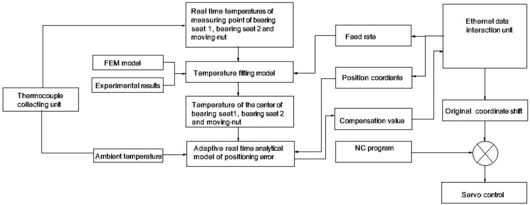
Configuration of the compensation system.

During working process, the temperature rise of four key points and axial positioning errors of the screw shaft were obtained with the four thermocouples and the laser interferometer, respectively. The four thermocouples are used to measure the real-time temperatures of bearing seat 1, bearing seat 2, the moving-nut flank, and ambient air. The FANUC FOCAS function was used to collect the real-time machine coordinate. According to the exponent fitting results, the key point temperatures of the screw shaft connecting with bearing 1, bearing 2, and the moving-nut were calculated using equations (33)–(35). Furthermore, the adaptive real-time positioning error was calculated according to equation (38). Finally, the calculated compensation value was sent to CNC system through the Ethernet data transmission unit in real time.

Compensation results

In this article, let $k = 43.3 {W / m}^{\circ} C$ and $ρ = 7800 kg / m^{3}$ .

The temperature distribution and thermal errors of ball screw feed drive systems were collected by an infrared thermal imaging instrument, thermocouples, and a laser interferometer. And, using the FOCAS library function for the FANUC digit control system, the real-time position of the moving-nut was collected.

Using thermocouple readings as inputs, the temperature fitting equation can be used to predict the temperature of the center of the kinematic pair in real time. The temperature equations for the bearing 1, bearing 2, and moving-nut are simultaneously obtained by this method.

In this work, the relationship between the measured point temperature and center temperature of heat sources is obtained using the FEM/Monte Carlo method and experiments. The FEM integrated with the Monte Carlo method is used to calculate the real heat generation rates of the bearing 1, bearing 2, and moving-nut, which are denoted by $Q_{B 1}$ , $Q_{B 2}$ , and $Q_{nut}$ , respectively. To get the three heat generation rates, an experiment was carried out to measure the temperature variations of 14 given points with time. The given points are denoted by $T 1$ , $T 2$ , …, and $T 14$ in Figure 5(a). The idea to determine the heat generation rates is that the measured temperatures of the given points match with the results obtained by the FEM/Monte Carlo simulation. The least squares of the differences between the measured and simulated results are used to match the measured and simulated results. That is, the solving process is to find the three parameters that minimize the following functional expression

F (Q_{B 1}, Q_{B 2}, Q_{nut}) = \sum_{m} \sum_{n} {(T_{mn}^{EXP} - T_{mn}^{FEM})}^{2}

where $T_{mn}$ denotes the temperature for given point $m$ at the nth sampling time step of $t_{n}$ , $m = 1, 2, \dots, 14$ , and $n = 1, 2, \dots, N$ , $T_{mn}^{EXP}$ denotes the measured value obtained by experiments, $T_{mn}^{FEM}$ denotes the simulated value obtained by the FEM/Monte Carlo method.

The solving process is showed as a flowchart in Figure 2. The Monte Carlo simulation can be used as a sampling process and will be repeated for a given sampling times p. The amount of p should be big enough to meet the calculation accuracy. Here, the function random( $H_{L}$ , $H_{U}$ ) of ANSYS APDL is used to generate a random number between $H_{L}$ and $H_{U}$ for the heat flow rate of each heat source.

After the FEM/Monte Carlo simulation is completed, the minimum objective function value meets a judgment criterion, then the calculation results of the heat generation rates are determined and the temperature field of the ball screw feed drive system is obtained.

From the obtained temperature field, the relationship between the measured point temperature and center temperature of heat sources is obtained, as shown in Figures 7 –9. In Figures 7(a), 8(a), and 9(a), the solid line denotes the center temperature of each heat source and the dash line denotes the surface measured temperature of each heat source. It is can be seen that the temperatures of three heat sources of bearing 1, bearing 2, and moving-nut always show a stable exponential increase under different feed rates, as shown in Figures 7(a), 8(a), and 9(a), which are similar to the results of Li et al.⁸

Figure 7.

(a) Temperature relationship between the measured point and the center of bearing 1 at feed rates of 0.3, 5, 10, and 15 m/min and (b) temperature difference between the measured point and the center of bearing 1 at feed rates of 0.3, 5, 10, and 15 m/min.

Figure 8.

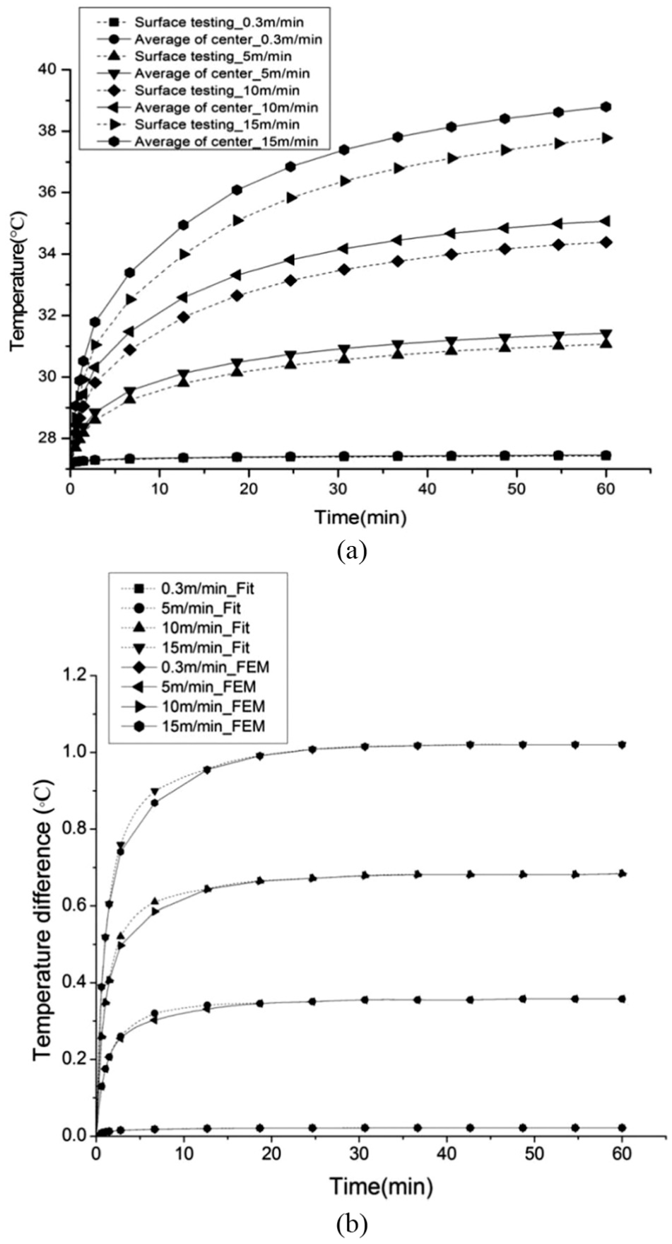
(a) T emperature relationship between the measured point and the center of bearing 2 at feed rates of 0.3, 5, 10, and 15 m/min and (b) temperature difference between the measured point and the center of bearing 2 at feed rates of 0.3, 5, 10, and 15 m/min

Figure 9.

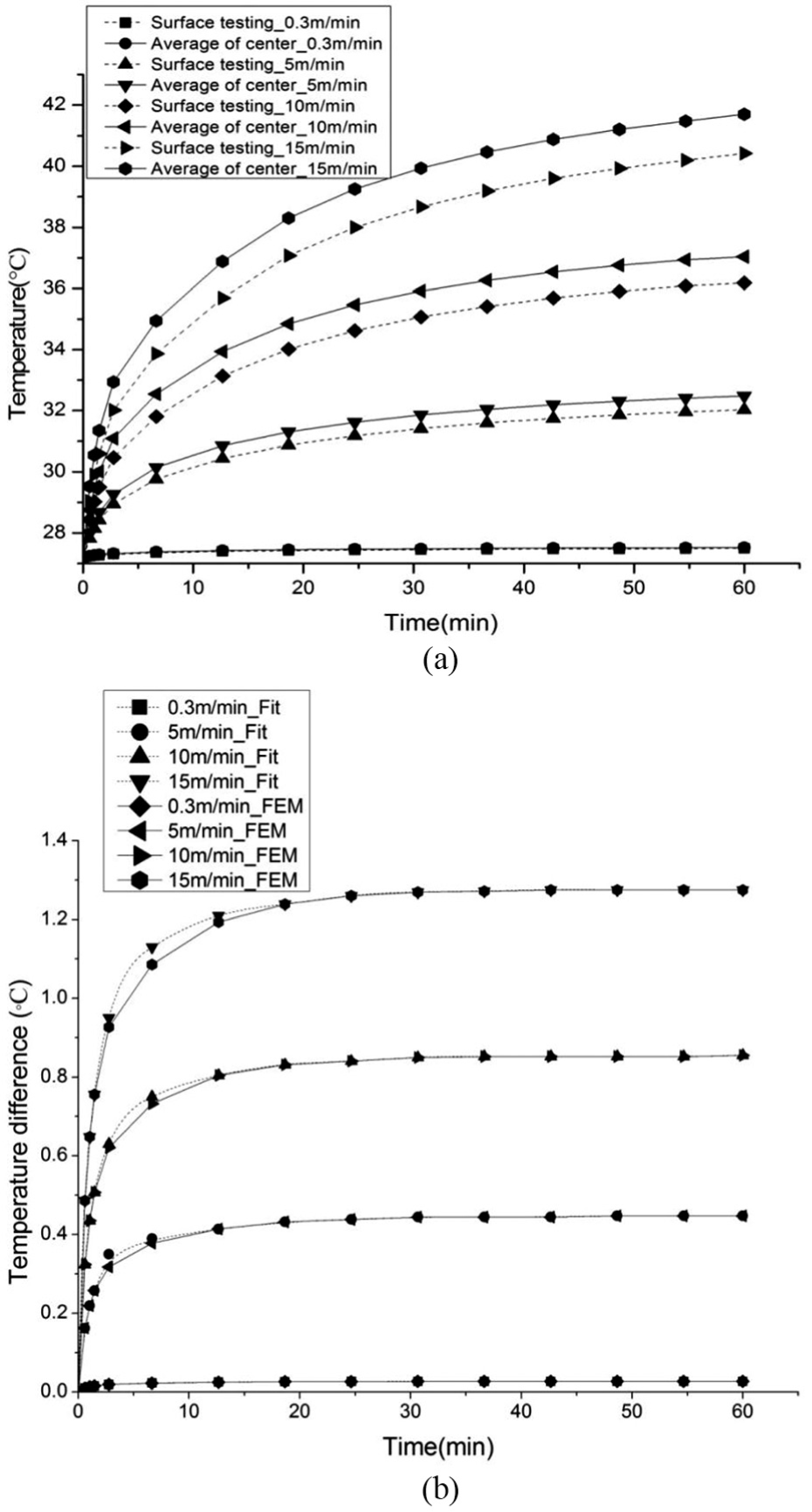
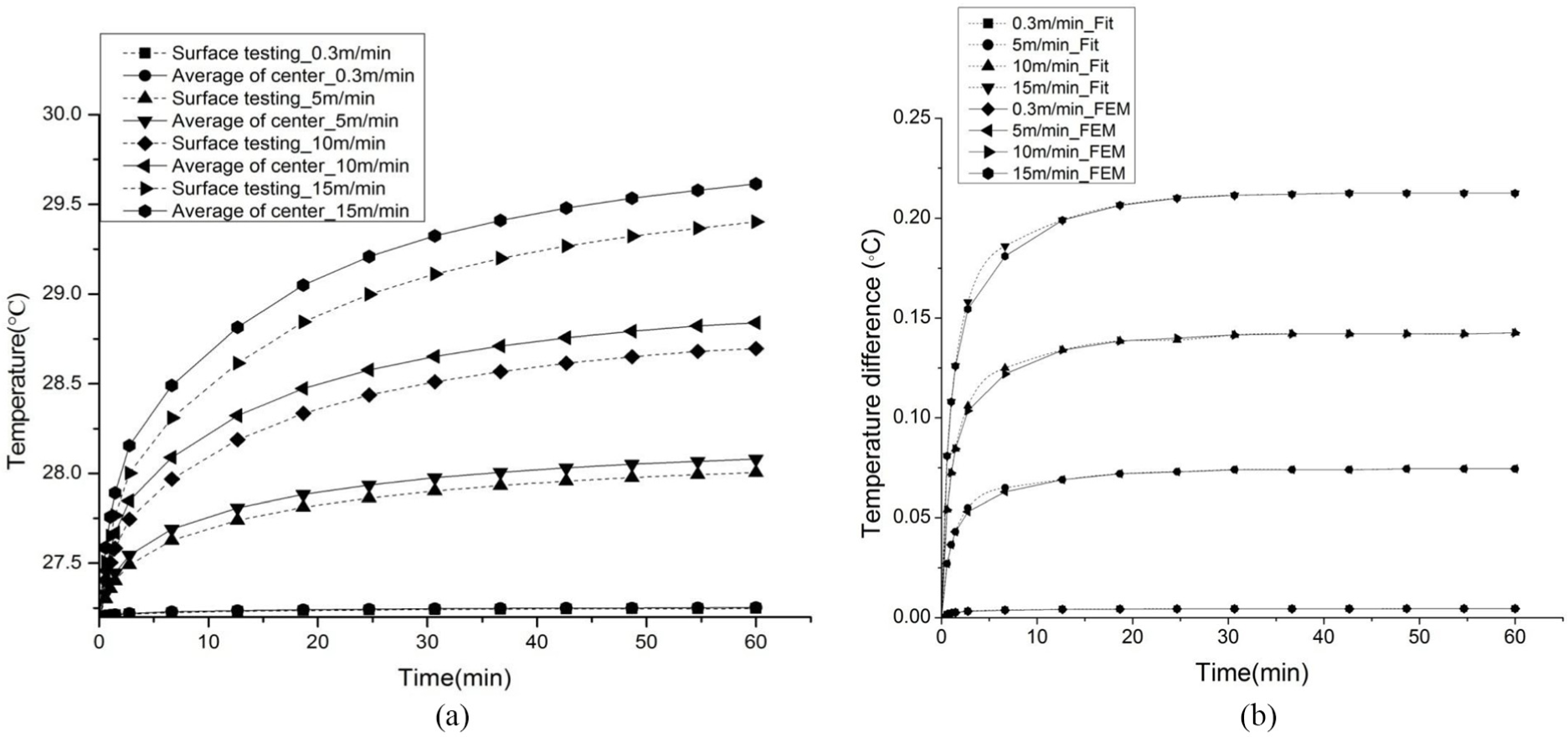
(a) Temperature relationship between the measured point and the center of moving nut at feed rates of 0.3, 5, 10, and 15 m/min and (b) temperature difference between the measured point and the center of moving nut at feed rates of 0.3, 5, 10, and 15 m/min.

In addition, in this work, the new findings are as follows:

The temperature difference between the measured point and the center of bearing 1, bearing 2, and moving-nut always shows a stable exponential rise under different feed rates, as shown in Figures 7(b), 8(b), and 9(b), respectively.

The stable rise of the temperature difference increases linearly as the feed rate increases.

Based on the above results, the equations for the temperature difference between the measured point and the center of each heat source can be fitted by an exponential function.

In equation (9), $C_{o 1}$ , $C_{o 2}$ , and $C_{o 3}$ are the constants obtained by exponential fit according to data of 5, 10, and 15 m/min feed rates, respectively. In this work, the constants of bearing 1, bearing 2, and the moving-nut are obtained, as shown in Table 3.

Table 3.

Constants of the fitting equation for the temperature difference.

Heat source	Constant
	$C_{o 1}$	$C_{o 2}$	$C_{o 3}$
Bearing 1	0.0662	−1.2208	19.8713
Bearing 2	0.0827	−1.2261	19.9507
Moving-nut	0.0138	−1.8472	29.2669

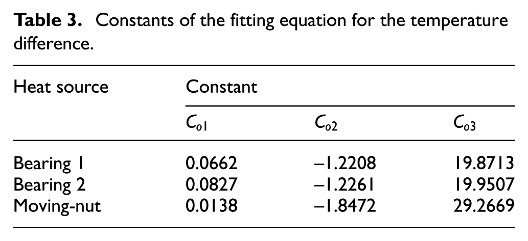
In Figures 7(b), 8(b), and 9(b), the solid line denotes the temperature difference obtained by FEM of each heat source and the dash line denotes the temperature difference obtained by fitting equation of each heat source.

From Figures 7(b), 8(b) and 9(b), the fitting results for the temperature difference under different feed rates agree with the results obtained by FEM. The maximum error is $0.08^{\circ} C$ . Furthermore, using the constants of Table 3, the fitting results for the temperature difference under the 0.3 m/min feed rate agree with the results of FEM. It is shown that the method is effective when it is applied on the cases out of the calibration range.

In Figure 10, the solid line denotes the temperatures of experiments and the dash line denotes the temperatures obtained by the present analytical model.

Figure 10.

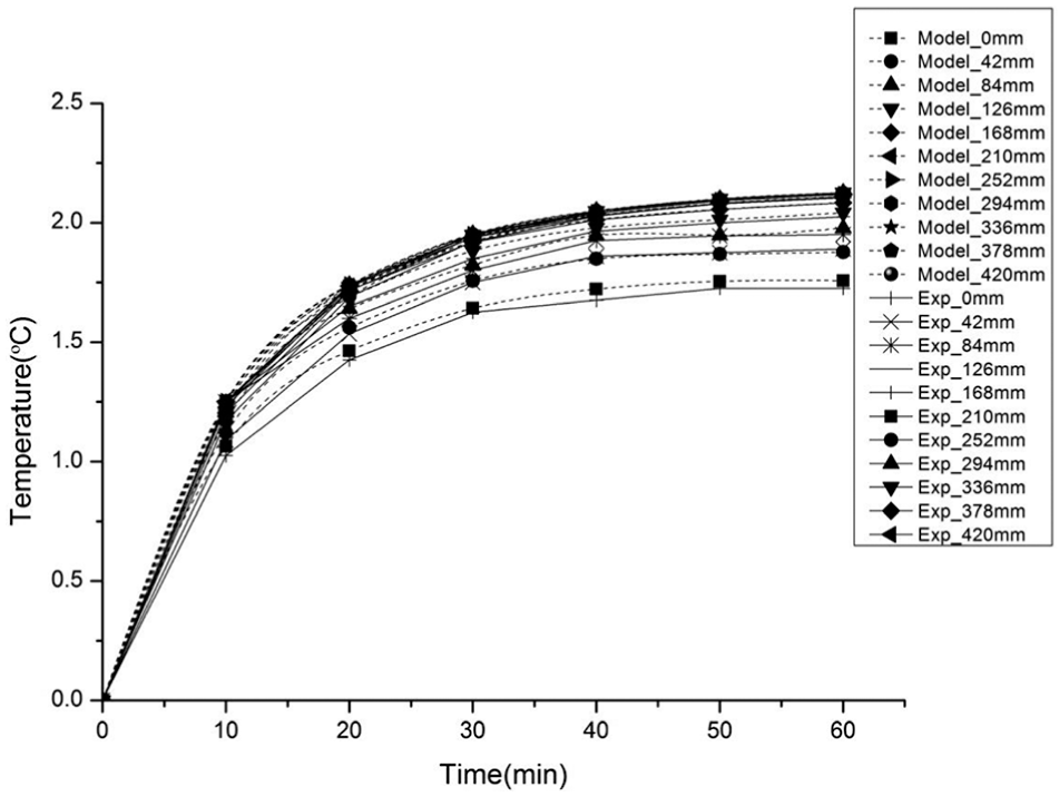
Comparison of the temperature rise obtained by the present analytical model and the experimental result under the feed rate 10 m/min.

Figure 10 shows that the temperature rise of analytical model agrees with that of experiments under the feed rate 10 m/min. In Figure 11, the solid line denotes the positioning error with compensation and the dash line denotes the positioning error without compensation.

Figure 11.

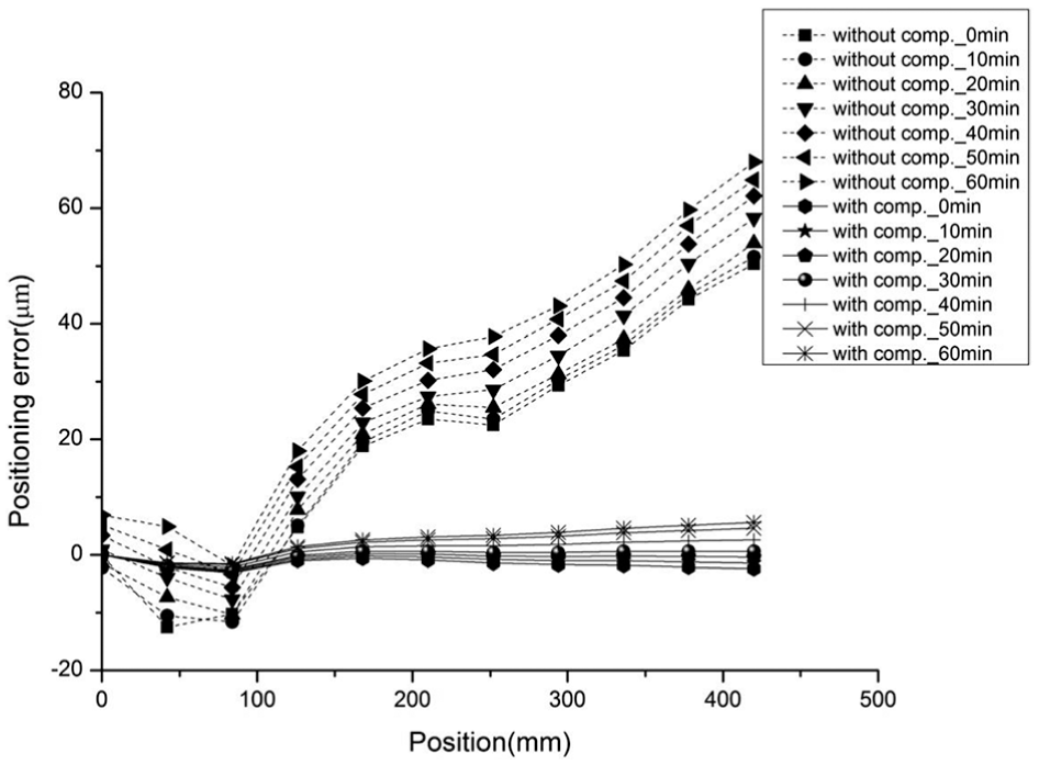
Comparison of positioning error between compensation and no-compensation under the feed rate 10 m/min.

Figure 11 shows the comparison of positioning error between compensation and no-compensation under the feed rate 10 m/min. The results show that the positioning error without compensation is high and the positioning error with compensation is low. The maximum value of axial thermal error shows a significant trend toward a decrease from 67 to 4 μm due to compensation. The effectiveness of proposed adaptive on-line analytical model is proved through the above results.

Conclusion

The positioning error compensation of z-axis of ball screw feed drive systems of the CNC lathe was investigated by an adaptive on-line analytical compensation model and experiments. From the results, the following conclusions can be drawn:

The FEM/Monte Carlo method developed in this work can be used to determine the real thermal boundary conditions of the ball screw feed drive system.

A new variable separation model of heat transfer is established based on the time and position exponential distribution functions. The model is used to calculate the transient temperature distribution of the screw shaft. And, the new model makes it possible to obtain the analytic solutions of complicated question on one-dimensional (1D) heat transfer.

The proposed adaptive on-line analytical compensation model based on the new variable separation model of multiple varying and moving heat sources is used to calculate the transient positioning error of the screw shaft and compensate the positioning error of ball screw feed drive systems in real time. This model has self-adaptive ability and robustness. By monitoring the temperatures of measured points of the bearing seats and moving-nut flank, this proposed method can realize on-line compensation for the positioning error of ball screw feed drive systems with multiple varying and moving heat sources. Therefore, the analytical model can satisfy the requirement of real-time compensation of the positioning error.

Footnotes

Appendix 1 Declaration of conflicting interests

The author(s) declared no potential conflicts of interest with respect to the research, authorship, and/or publication of this article.

Funding

The author(s) disclosed receipt of the following financial support for the research, authorship, and/or publication of this article: This work was supported by the National Natural Science Foundation of China under Grant No. 51375081. This work was also supported by the Important National Science & Technology Specific Projects “High-end CNC machine tools and basic manufacturing” of China under Grant No. 2013ZX0401-011.

ORCID iD

Chun-yu Zhao,

References

Liu

Lyu

SK.

Study on thermal behavior analysis of nut/shaft air cooling ball screw for high-precision feed drive. Int J Precis Eng Man 2014; 15(1): 123–128.

Liu

Sun

et al . Comprehensive thermal compensation of the servo axes of CNC machine tools. Int J Adv Manuf Tech 2016; 85(9): 2715–2728.

Shi

Zhang

Yang

et al . Experiment-based thermal error modeling method for dual ball screw feed system of precision machine tool. Int J Adv Manuf Tech 2016; 82(9): 1693–1705.

Dai

Wang

Xiong

et al . Thermal error modelling of motorised spindle in large-sized gear grinding machine. Proc IMechE, Part B: J Engineering Manufacture 2017; 231(5): 768–778.

Yang

Fan

et al . Integrated geometric and thermal error modeling and compensation for vertical machining centers. Int J Adv Manuf Tech 2015; 76(5): 1139–1150.

Liu

Sun

et al . Spindle axial thermal growth modeling and compensation on CNC turning machines. Int J Adv Manuf Tech 2016; 87(5–8): 2285–2292.

Min

Jiang

A thermal model of a ball screw feed drive system for a machine tool. Proc IMechE, Part C: J Mechanical Engineering Science 2011; 225: 186–193.

Fan

Yang

et al . Time-varying positioning error modeling and compensation for ball screw systems based on simulation and experimental analysis. Int J Adv Manuf Tech 2014; 73(5–8): 773–782.

Yang

Feng

Zhao

et al . Thermal error modeling and compensation for a high-speed motorized spindle. Int J Adv Manuf Tech 2015; 77(5–8): 1005–1017.

10.

Mou

A method of using neural networks and inverse kinematics for machine tool error estimation and correction. Journal of Manuf Sci E-T ASME 1997; 119(2): 247–254.

11.

Chi

Zhao

Mei

et al . Thermal error modeling of machine tool spindle based on particle swarm optimization and neural network. J Shanghai Jiaotong Univ 2016; 50(5): 686–694 (in Chinese).

12.

Wang

et al . Thermal error prediction of the spindle using improved fuzzy-filtered neural networks. Proc IMechE, Part B: J Engineering Manufacture 2016; 230(4): 770–778.

13.

Kang

Chang

Huang

et al . Modification of a neural network utilizing hybrid filters for the compensation of thermal deformation in machine tools. Int J Mach Tool Manu 2007; 47(2): 376–387.

14.

Zhang

Yang

Jiang

Machine tool thermal error modeling and prediction by grey neural network. Int J Adv Manuf Tech 2012; 59(9–12): 1065–1072.

15.

Zhang

Guo

et al . Thermal error optimization modeling and real-time compensation on a CNC turning center. J Mater Process Tech 2008; 207(1–3): 172–179.

16.

Liang

Zhang

Yang

The thermal error optimization models for CNC machine tools. Int J Adv Manuf Tech 2012; 63(9–12): 1167–1176.

17.

Liu

Sun

et al . Thermal error modeling method for a CNC machine tool feed drive system. Math Probl Eng 2015; 2015: 436717.

18.

Han

Wang

Cheng

A new thermal error modeling method for CNC machine tools. Int J Adv Manuf Tech 2012; 62(1–4): 205–212.

19.

Vyroubal

Compensation of machine tool thermal deformation in spindle axis direction based on decomposition method. Precis Eng 2012; 36(1): 121–127.

20.

Zhang

Shan

Application of sliced inverse regression with fuzzy clustering for thermal error modeling of CNC machine tool. Int J Adv Manuf Tech 2016; 85(9–12): 2761–2771.

21.

Yan

Yang

JG.

Application of synthetic grey correlation theory on thermal point optimization for machine tool thermal error compensation. Int J Adv Manuf Tech 2009; 43(11–12): 1124–1132.

22.

Ramesh

Mannan

Poo

AN.

Support vector machine model for classification of thermal error in machine tools. Int J Adv Manuf Tech 2002; 20(2): 114–120.

23.

Miao

Gong

Niu

et al . Robustness of thermal error compensation modeling models of CNC machine tools. Int J Adv Manuf Tech 2013; 69(9–12): 2593–2603.

24.

Lee

Yang

SH.

Thermal error modeling of a horizontal machining center using fuzzy logic strategy. J Manuf Process 2001; 3(2): 120–127.

25.

Yao

Chen

ZC.

Bayesian networks modeling for thermal error of numerical control machine tools. J Zhejiang Univ-Sci A 2008; 9(11): 1524–1530.

26.

Mian

Fletcher

Longstaff

et al . Efficient estimation by FEA of machine tool distortion due to environmental temperature perturbations. Precis Eng 2013; 37(2): 372–379.

27.

Zhao

et al . Thermal error modeling of the spindle based on multiple variables for the precision machine tool. Int J Adv Manuf Tech 2014; 72(9–12): 1415–1427.

28.

Mayr

Ess

Weikert

et al . Compensation of thermal effects on machine tools using a FDEM simulation approach. In: Proceedings of the Lamdamap 9th international conference, London, 29 June–2 July 2009, pp.38–47. Sieca Repro.

29.

Wang

Zhang

Yang

et al . Geometric and thermal error compensation for CNC milling machines based on Newton interpolation method. Proc IMechE, Part C: J Mechanical Engineering Science 2013; 227(4): 771–778.

30.

Wang

Liu

Kang

An efficient error compensation system for CNC multi-axis machines. Int J Mach Tool Manu 2002; 42(11): 1235–1245.

31.

Xiang

Yang

Thermal error prediction method for spindles in machine tools based on a hybrid model. Proc IMechE, Part B: J Engineering Manufacture 2015; 229(1): 130–140.

32.

Liu

Sun

et al . Thermal error compensation without temperature sensors for CNC machine tools’ feed drive system. J Mech Eng 2016; 52(15): 162–169 (in Chinese).

33.

Tanabe

Takada

Thermal deformation of machine tool structures using resin concrete. T Jpn Soc Mech Eng C 1994; 37(2): 384–389.

Adaptive on-line compensation model on positioning error of ball screw feed drive systems used in computerized numerical controlled machine tools

Abstract

Keywords

Introduction

FEM model integrated with theMonte Carlo method

Heat transfer coefficient

Implementation of the FEM model

Temperature distribution rule between the measured point and the center of heat sources

Adaptive analytical model of the positioning error

Equation of heat conduction of multiple varying and moving heat sources

Thermal error of the screw shaft

Positioning error of the screw shaft

Experimental details

Experimental setup

Testing procedure

Real-time compensation of the positioning errors

Compensation method

Compensation results

Conclusion

Footnotes

Appendix 1

Declaration of conflicting interests

Funding

ORCID iD

References