
Abstract
A generalized mechanical model is proposed to predict cutting forces for five-axis milling process of sculptured surfaces with generalized milling cutter, which is considered as a revolution around tool axis of an arbitrary section curve composed of variable lines and curves. Solid-analytical-based method is presented and extended to precisely and efficiently identify the cutter–workpiece engagements between the generalized milling cutter and workpiece being machined. And the undeformed chip thickness is calculated with respect to pre-defined tool coordinate system, which is regarded as the transformation form of feed cross–feed normal system by lead and tilt angles. Although only two experimental validations (peripheral milling with cylinder end mill and multi-axis milling with ball end mill) are performed to estimate the robustness and flexibility of the method presented, it can be applied for an arbitrary mill geometry in multi-axis milling as well as three-axis milling, two-and-a-half-axis milling. Finally, a case study of aero-engine impeller five-axis milling with ball end mill is performed to further illustrate the validation of the model.
Keywords
Introduction
Due to the excellent machining flexibility, multi-axis milling technologies are playing more and more important roles in machining process of parts with sculptured surfaces, such as the ones designed in aerospace, automotive, die and mold industries. Selection of cutting parameters is very crucial to achieve increased productivity and part quality in such industries, where high cost of raw material, equipment, and tooling involved. 1 However, multi-axis milling also brings additional challenges because of the complexity of cutter–workpiece geometry and process parameters. Chatter vibration and tool deflection due to the dynamic interactions between tool and workpiece are typical challenges in multi-axis milling process which have a close relation with the cutting force. 2
Cutting force is an important fundamental parameter in the machining process. Many research works are conducted based on evaluating cutting forces. A method to analyze the three-dimensional (3D) tool deflection and the surface form error in three-axis ball end milling was presented based on cutting forces. 3 A method for real-time estimation of tool wear in face milling was presented based on cutting force signals. 4 The influence of cutting forces on machining of Inconel 718 curved surface and optimized cutting parameters was studied. 5 A method for 3D chatter stability prediction of milling was demonstrated based on the liner and exponential cutting force model. 6 At present, a method for accurate surface roughness prediction in end milling operation for intelligent machining was presented using cutting forces–based adaptive neuro-fuzzy approach. 7 A geometric envelope approach with two major distinctions was proposed to calculate the envelope surface in five-axis milling. 8 From the literature review presented above, it can be seen that the cutting forces are the essential variables and links in milling process, especially for multi-axis milling process, which relate the material removal process to workpiece surface quality.
Therefore, extensive amount of work has been done by researchers on the modeling cutting force in milling process. In the early years, a cutting force model with helical ball end mill was presented, 9 which was based on the establishment of a database containing basic machining quantities evaluated from a set of standard orthogonal cutting tests. An explicit expression of cutting force in peripheral milling of curved surfaces was proposed, which included the effect of workpiece curvature.10,11 Afterward, using orthogonal to oblique transformation, an enhanced mathematical model for calculating cutting forces was developed in order to improve cycle time in sculptured surface machining, 12 and a cutting force model for five-axis milling operations was presented, where the effect of inclination angle was considered. 13
In order to model the cutting force, the extraction of the cutter–workpiece engagement (CWE) is a key procedure. For multi-axis milling, however, it is difficult to identify the CWE due to the complexity of cutting process, which cannot be generally performed using analytical method. 14 For the relative simple cutting cases, the engagement regions were analytically determined and the cutting forces were modeled. 13 An analytical methodology for determining the shapes of the cutter swept envelopes was developed, 15 in which cutter surfaces performing five-axis tool motions were decomposed into a set of characteristic circles, and the concept of two-parameter family of spheres was introduced to obtain these circles. A boundary representation (B-rep)–based exact Boolean method was presented for extracting complex CWE as every cutter location point. 16 All the analytical methods need a lot of professional and expert backgrounds in mathematics and graphics. They are also lack of flexibility and robustness in some complex cutting operations. Therefore, the analytical method is not the good choice on the viewpoint of efficient, cost, and so on. And many non-analytical methods were presented to extract the CWE for multi-axis milling, such as the solid modeling method17,18 and the discrete modeling method (e.g. Z-buffer method19–22). For both the approaches, in order to keep track of the material removal, the workpiece update is necessary. Therefore, larger computer memory capacity is required, which is in proportion to both resolution of description and scale of workpiece. Recently, the CWEs for complex multi-axis cases were calculated by the general projective geometry approach, where the cutting tool envelope and the cutting edges were represented as organized point clouds. 23 However, the cutting force coefficient identification is also an essential work to model cutting force because the mechanistic model is commonly used in present academic researches and industrial applications. The common approaches include finite element method, 24 experimental method through variable feed, 25 and transformation from orthogonal to oblique. 26 The cutting forces in end milling operations were simulated using finite element method based on Johnson–Cook theory. 24 The calculation process of actual cutting force coefficients was proposed based on the imprecise estimation of cutting force coefficients in milling of thin-walled part using cutter with different tooth radii. 27 For multi-axis milling process, due to the complex of milling cutter, cutting force coefficient is generally identified through transformation from orthogonal to oblique.
Additionally, the influence of several parameters on cutting force and optimization of cutting parameters based on cutting force model was studied in many articles for multi-axis milling process. The effects of tool–surface inclination on cutting forces in ball end milling were studied. 28 A cutting forces model based on geometric analysis was presented, 29 and the relationships among undeformed chip thickness, rake angle, cutting velocity, shear plane area, and chip flow angle in ball end milling were clearly described. The 3D cutting forces in the tool axis system were obtained by minimum energy method. A method to model and predict the instantaneous cutting forces in five-axis milling processes with radial cutter runout was presented based on tool motion analysis. 30 The optimal feed directions and analytical solutions for the optimal tool orientations in five-axis flat-end milling of spherical, cylindrical, and toroidal surfaces were identified based on a given cutter contact point. 31 Cutter posture stability graph was presented to achieve chatter avoidance without the trouble of tuning other process parameters in five-axis milling process. 32 At present, a new approach was presented to integrate the cutter runout effect into envelope surface modeling and tool path optimization for five-axis flank milling with a conical cutter.33,34 In this methodology, the cutting tool envelope is defined as a revolved surface of a multi-segmented section, which is composed of arcs and lines.
Nonetheless, majority of the above works limited to three-axis milling process and the existing cutting force model are mainly focused on single milling tool shapes, for example, ball end mill, except for the mechanistic model proposed based on the envelope of milling tool defined by seven geometric parameters. 35 Additionally, the five-axis milling impeller is a classical application of multi-axis machining. The work related to this field is rare except for the optimal geometry of conical tool in five-axis flank milling of impellers 36 and the feedrate scheduling for multi-axis plunge milling of open blisks. 37 The author presented a solid-analytical-based method (SAM) for extracting CWE in sculptured surface milling using ball end mill, which can be used to predict the cutting force multi-axis milling process. 38 In this article, the method presented in Ju et al. 38 is employed and extended to develop a generalized milling force model for multi-axis milling with generalized milling cutter. And application of the model in an aero-engine impeller five-axis milling is performed in detail.
Geometry of generalized milling cutter
With the advancements in manufacturing and material in recent years, more and more milling cutters are appeared with different shapes, especially for some specific use in aerospace, die-mold, and automobile industries, where complex surfaces and geometries are machined. Modeling of cutting forces in multi-axis milling requires the milling cutter to be geometrically defined, so in this section, the geometry of generalized milling cutter is constructed.
Coordinate frames
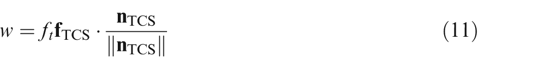
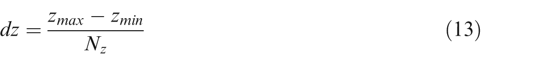
Three coordinates (as shown in Figure 1(a)), namely, global coordinate system (GCS), feed cross–feed normal system (FCN), and tool coordinate system (TCS) are necessary to precisely define the spatial motion of cutting cutter in multi-axis milling operations. GCS composed of three axes X, Y, and Z is a fixed coordinate system, the origin and orientation of which are arbitrary. FCN, consists of feed (F), cross-feed (C), and surface normal (N) axes, is a moving coordinate, or called process coordinate. The FCN coordinate is moving with the cutting cutter along the tool path, the origin of which is in the end of cutting tool. Thus, the position and orientation of FCN coordinate mainly depend on feed direction, normal of the machined surface, and the position of cutting tool. TCS made up of x, y, and z axes is the last coordinate, the origin of which coincide with FCN.
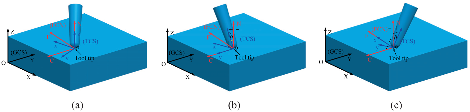
Geometry of five-axis milling: (a) coordinate systems, (b) lead angle α, and (c) tilt angle β.
From Figure 1, the rotation matrix
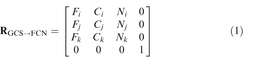
where
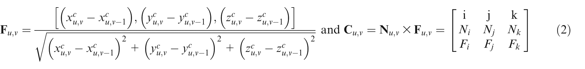
Here,
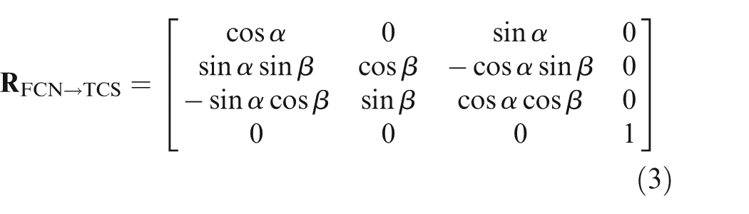
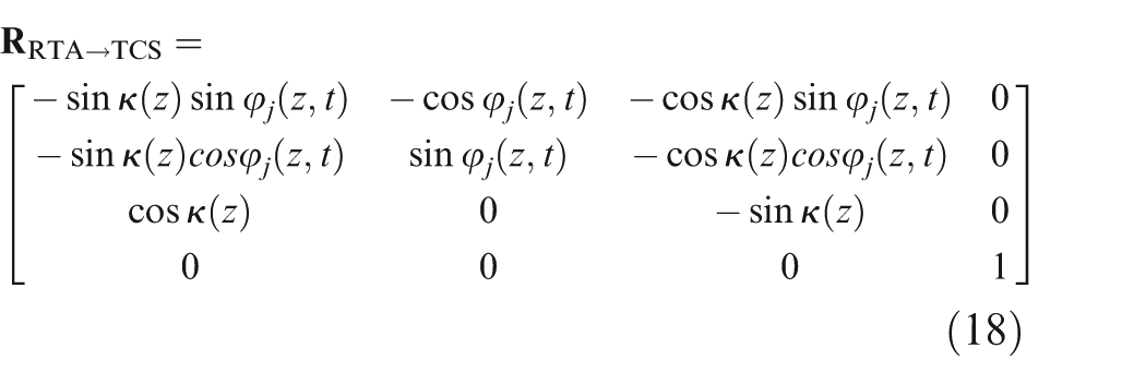
where α and β are lead and tilt angles, respectively, as shown in Figure 1.
It should be noted that two files (CL file and CN file) are required in equations (1) and (2). The CL file can be easily obtained with the help of commercial computer-aided manufacturing (CAM) software. So the tool tip position, tool orientation, and process parameters, such as feed velocity and cutting speed can be extracted in GCS coordinate from the CL file. Moreover, if lead angle α = 0, tilt angle β = 0, and keep all other process parameters same as the original CL file, a CN file can be obtained, which can be used to present the surface normal vectors,
Generalized milling cutter profile
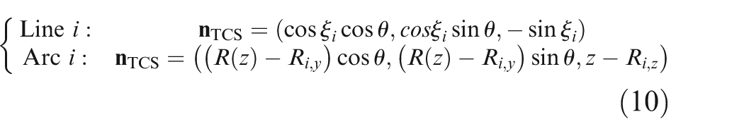
In the early years, automatically programmed tool (APT) and computer-aided design and computer-aided manufacturing (CAD/CAM) systems defined the envelope of milling tool by seven geometric parameters. 35 However, the way using seven geometric parameters for the definition of milling tools is limited with the rapid development of manufacturing technology, especially for the appearance of non-standard milling cutter. Although there are a large number of milling cutters with different shapes used in practical manufacture, all of the cutters can be considered as revolutions of arbitrary section curves around the tool axis, resulting in volumetric tool envelopes. In this article, the generalized milling cutter’s section curve is defined by a combination of lines and arcs shown in Figure 2(a). All the lines can be defined by two points—starting point Li1 and ending point Li2—and the inclination angle ξi and all the arcs can be defined by the center oi and radius Ri of the arcs. It should be noted that the line and arc may be not tangent at the connective point between the connected lines and arcs.
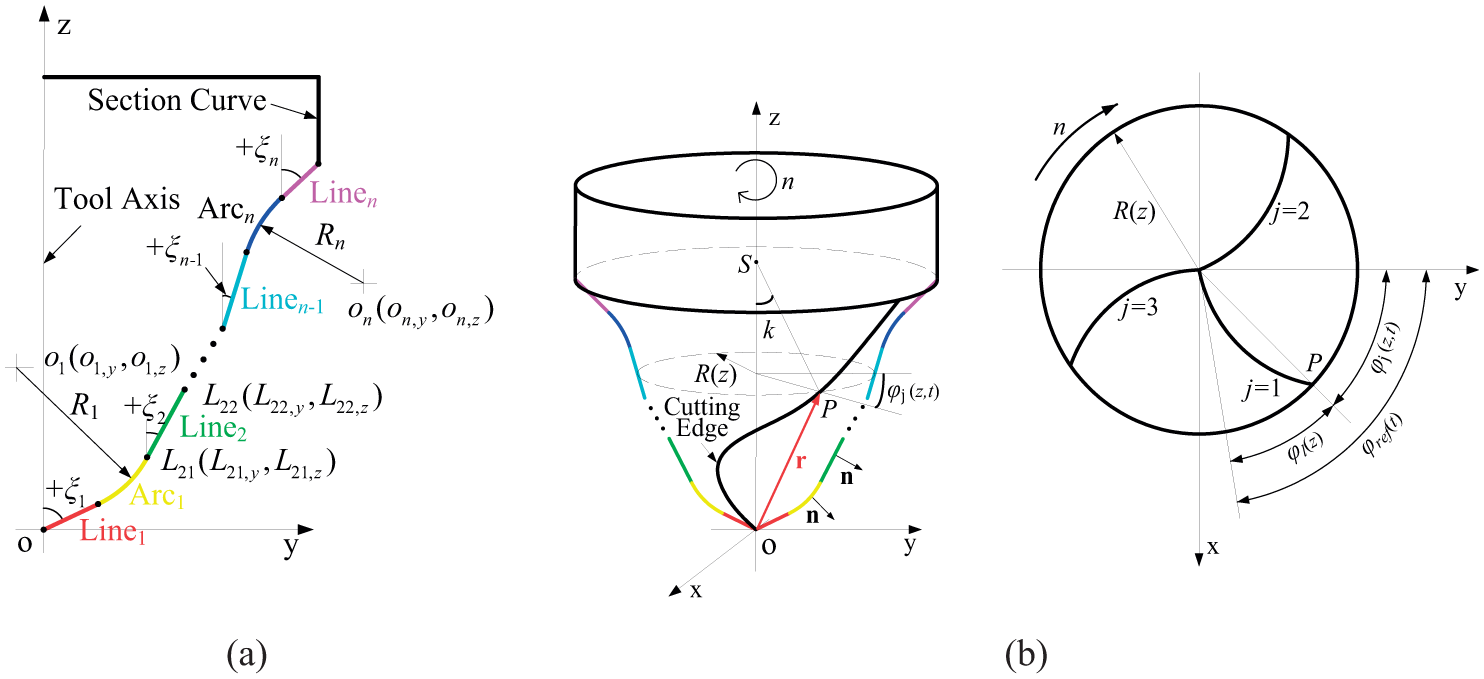
Geometry of generalized milling cutter: (a) section curve and (b) cutter geometry.
The generalized section curve presented above can define a variety of standard and non-standard milling cutter profiles, such as cylinder end mill, ball end mill, taper ball end mill, and bull nose end mill. The section curves of them are composed of lines and arcs, and different milling cutter profiles have different configurations. And two key parameters, inclination angle ξ and radius R, which are considerably important to define the cutting edges are also shown in these figures.
Geometry of cutting edge
Helical flutes can be wrapped around the cutters around the milling tool shown in Figure 2(b). A point P on the helical flute is characterized by elevation z, local radius R(z), axial immersion angle κ(z), and radial immersion angle φj(z,t). A vector drawn from the origin of TCS to point P can be expressed as

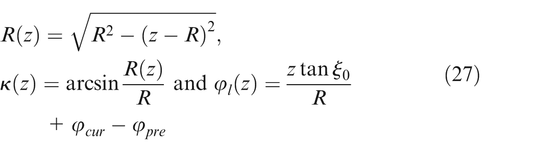
The local radius R(z) depends on the geometry of the cutter envelope. At the tool tip, the local radius R(z) is zero and changes along z-axis, which can be described as
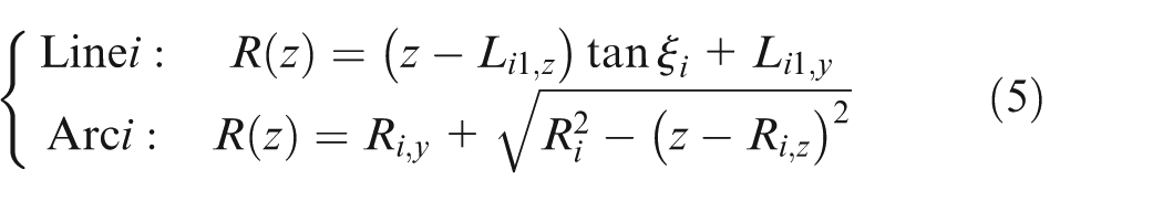
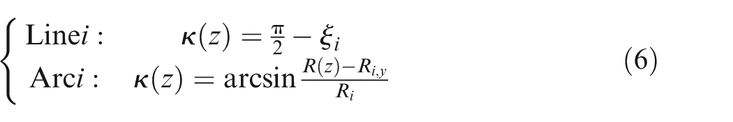
where ξi and Li1(Li1,y, Li1,z) are the inclination angle and starting point of line i, respectively, as shown in Figure 2(a). oi(Ri,y, Ri,z) is the center of arc i, and Ri is the radius of arc i. Axial immersion angle κ(z) is the angle between tool axis and cutting edge normal and is given as follows
For general milling cutters with variable helix and variable tooth pitch separation, the generalized radial immersion angle φj(z,t) for the jth cutting edge is written as follows

where φp is the pitch angle of the jth cutting edge with respect to the previous (j−1)th one. φref(t) is the angular position of the reference cutting edge measured on the x-y plane between the positive y direction and the tangent line of the cutting edge at the tool tip and can be calculated as

where φ0 is the initial angular position of the cutting tool, n is the rotational speed of the cutting tool, dt is the time interval, dt = T/NT. T is total time length of one cut, and NT is the number of time discretization. φl(z) is the lag angle of the point P on the cutting edge measured on the x-y plane. The mill cutter is generally constant lead or constant helix, so φl(z) has different expression. The constant helix, which leads to variable lead along the cutting edge, has uniform cutting mechanics. Therefore, in this article, the constant helix is molded here, and the φl(z) can be calculated as
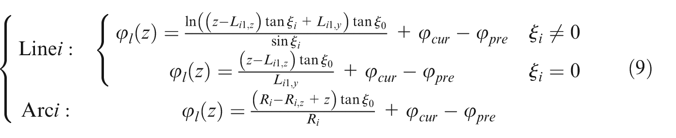
where ξ0 is the constant helix angle of the milling tool. φcur and φpre are the lag angle of current segment at its starting point and the final lag angle of the previous segment at the starting point of the current one, respectively.
Surface normal of the milling tool is an important parameter for the determination of swept regions in the process of CWE calculation in multi-axis milling. Surface normal of the generalized milling tool in TCS, shown in Figure 2(b), can be expressed as
where θ is the circumferential position of the cutting tool, θ ∈ [0,2π].
Generalized cutting force model
Cutting force is an important fundamental input data for the tool deflection, form accuracy calculation, tool breakage detection, and process optimization. Compared with three-axis milling, cutting forces in multi-axis milling process are more complicated. The varying CWE, lead, and tilt angles along tool path are the main challenges in the process of cutting force calculation in multi-axis milling process. In this section, a generalized cutting force model is developed based on traditional mechanical model, which contains undeformed chip thickness model and cutting force model.
Undeformed chip thickness
CWE extraction can be performed using the SAM presented in Ju et al.
38
based on two kinds of cutting cases (the first cut/slotting case and the following cut case), the robustness and flexibility of which have been verified through milling experiments. The procedures for extracting CWE can be simply summarized as follows: (1) cutting tool and raw stock are modeled first by commercial CAM software, and the possible CWEs are obtained by performing Boolean subtraction operations between them at any CLs. (2) For the first cut or slotting cases, the exact CWEs are obtained performing
During the machining process of sculptured surface, the undeformed chip thickness is difficult to evaluate because local chip thickness is variable along the cutting flute depending on the immersion angle and z coordinate as presented in Figure 3. Many researchers25,39 assumed that the feed vector is in coincidence with the x axis to define the TCS; in this case, the undeformed chip thickness can be easily calculated using a simple expression. However, using this definition, lead and tilt angles which are two important parameters in multi-axis milling are difficult to be determined because TCS mainly depends on the tool axis vector and feed vector. As a matter of fact, TCS is the rotated form of FCN by lead angle α and tilt angle β as presented in equation (3). Therefore, undeformed chip thickness can be calculated in TCS
where ft is feed per tooth,

where
Cutting force model.
Cutting force model
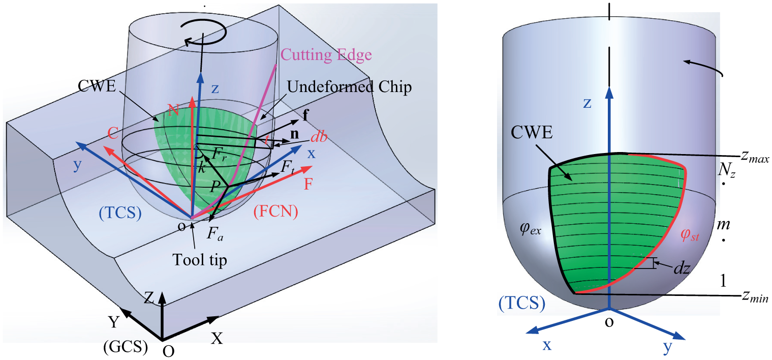
In multi-axis milling process, the cutting geometry and cutting parameters are variable along the tool path. In the process of calculating cutting forces, the engaged cutting edges are decomposed into a series of elementary cutting edges corresponding to the CWE discretization. The element height dz (Figure 3) is determined by the scope of CWE along tool axis and the number of discretization Nz and can be expressed as
where zmax and zmin are the maximum and minimum z coordinates of the CWE in TCS, respectively.
According to the traditional mechanical model, which includes the shearing and plowing mechanism in the cutting process, radial Fr,lmj(z,t), tangential Ft,lmj(z,t), and axial Fa,lmj(z,t) differential cutting forces at the lth time interval, mth element on the jth cutting tooth in TCS can be expressed as
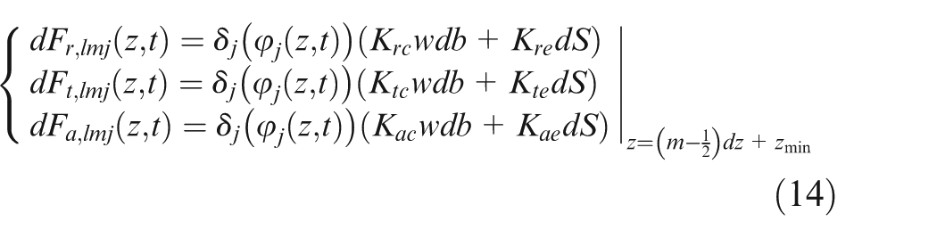
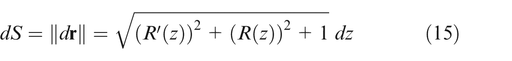
where Krc, Ktc, and Kac are the cutting force coefficients contributed by the shearing action in radial, tangential, and axial directions, respectively; Kte, Kre, and Kae are the edge force coefficients, which are determined using the mechanics of milling method.26,40 In this approach, parameters required for the calculation of cutting force coefficients are obtained from an orthogonal cutting database. w is the uncut chip thickness of the selected element in the normal direction of the cutting tool. db is the differential width of chip thickness and can be calculated by db = dz/(sinκ). dS is the differential cutting length of cutting edge can be calculated using equation (4) as
δj(φj(z,t)) is a rectangular window function that assumes a value one when the cutting tooth j is engaged in the cutting process and zero when the cutting tooth is out of cut
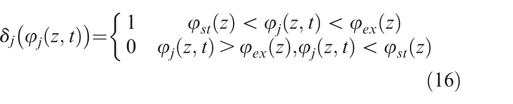
where φst(z) and φex(z) are the start cutting and exit cutting angles for the tooth with respect to z coordinate, respectively, and the values of elementary φst(z) and φex(z) are obtained from the CWE data.
The differential cutting forces in radial, tangential, and axial directions can be transformed into the TCS as follows
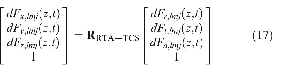
where
The total cutting force acting on the cutting tool is calculated by summing up the differential cutting forces contributed by the Nz discretized elements and the engaged cutting flute as follows
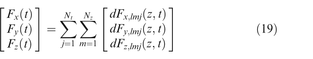
where Nt is the number of cutting edges.
As the measured cutting forces using the dynamometer in experiment are in GCS, in order to testify the validity of the cutting forces predicted, the predicted cutting forces must be transformed into the GCS, and the transformation process can be expressed as
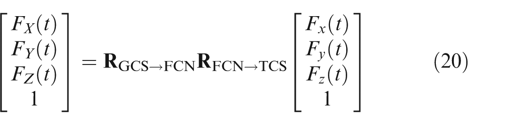
where rotation matrices
It should be noted that milling tool used is a generalized milling cutter in above section. To sum up, the algorithm in one-cut operation for cutting force prediction with generalized milling tool using SAM for CWE extraction is shown Figure 4. The algorithm can be implemented on the platform of MATLAB, and the validity of the algorithm is verified in next section.
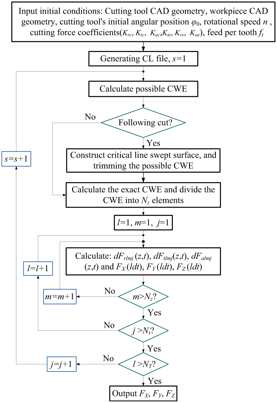
Flowchart for cutting force calculation.
Validations and application
First, to verify the efficiency and accuracy of the generalized mechanical model proposed in above section, two milling cases with cylinder end mill and ball end mill are employed to perform the cutting force prediction, as well as the comparison of cutting forces obtained by analytical and experimental methods are conducted. And then, a key application of an integrated impeller part milling using five-axis machine tool is illustrated to evaluate the flexibility of the cutting force model.
Validation I: peripheral milling with cylinder end mill
The first validation example is peripheral milling with cylinder end mill, where the cutting force model has been reported in many classical literatures.6,9,25,26 According to the geometries of cylinder end mill, the parameters are ξ1 = 90° and ξ2 = 0° in this case. Thus, section curve revolted to form cutter profile, contains only two lines, and L11(L11,y, L11,z) = L11(0, 0) and L12(L12,y, L12,z) = L12(R, 0) for Line 1, L21(L22,y, L21,z) = L22(L22,y, L22,z) = L22(R, z) for Line 2, where R is radius of cutter. According to equations (5), (6), (9) and (10)
For Line 1

and

For Line 2
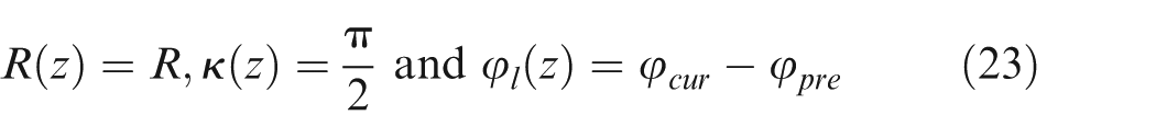
and

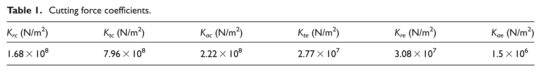
Substituting equations (22) and (24) into equations (11) and (14), the cutting forces can be calculated. Figure 5 shows the cutting forces evaluated by analytical method presented and experimental measurement (using Kistler-type 9257B dynamometer). Here, a cemented carbide cylinder end mill with four flutes, 12 mm diameter, 45° helix angle is used, and the workpiece material is 7050 aluminum alloy. The cutting force coefficients are listed in Table 1. The cutting parameters are as follows: spindle speed is 2000 r/min, axial depth of cut is 4 mm, radial depth of cut is 2 mm, and feed per tooth is 0.1 mm. A good agreement between the analytical and experimental results can be observed clearly.
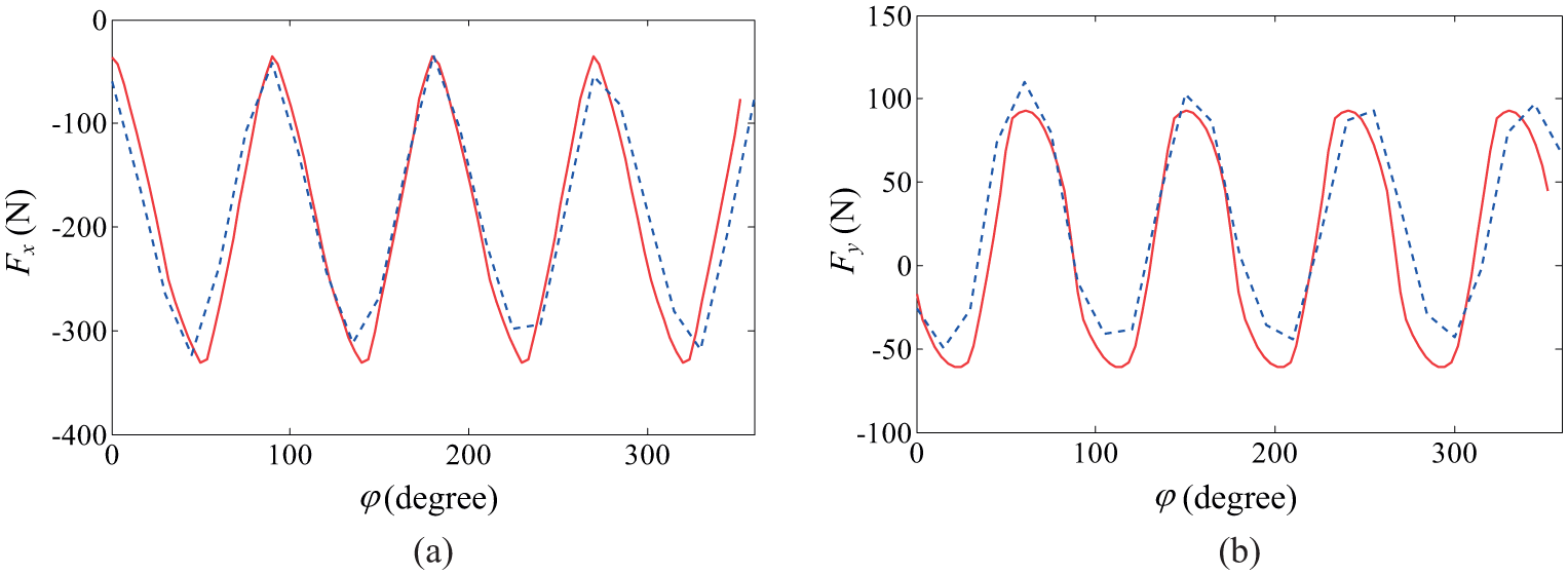
Cutting forces for peripheral milling with cylinder end mill (red solid lines: calculated force; blue dashed lines: measured force): (a) cutting force in x direction and (b) cutting force in y direction.
Cutting force coefficients.
Validation II: multi-axis milling with ball end mill
The second example is a milling process with ball end mill with assumption of constant lead and tilt angles. Similar with the analysis presented above, for ball end mill, R1 > 0 and ξ2 = 0°. Thus, section curve revolted to form cutter profile contains one arc and one line, and the center o1(R1,y, R1,z) = o1(0, R) and L11(L11,y, L11,z) = L11(R, z). According to equations (5), (6), (9) and (10)
For Line 1
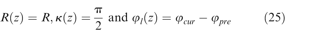
and

For Arc 1
and

Substituting equations (26) and (28) into equations (11) and (14), the undeformed cutting thickness and the cutting forces can be calculated. Different with the peripheral milling with cylinder end mill, it should be noted that the CWEs need to be identified using numerical method due to the complexity of cutting process. Here, the SAM presented in Ju et al. 38 is employed. Additionally, due to the representative of the following cutting (non-first cutting), here only following case is considered. And cutting parameters are as follows: spindle speed is 5000 r/min, feed per tooth is 0.05 mm, depth of cut is 4 mm, and step over is 3 mm. In cutting tests, a cemented carbide ball end mill with two flutes, 10 mm diameter, 35° helix angle is used, and the workpiece material is aluminum alloy. The cutting force coefficients are shown in Table 1. Four cases (Case_A ∼ Case_D as shown in Table 2) with different lead and tilt angles are included here. The lead and tilt angles are, respectively, fixed as 10° for these four cases.
Comparisons of CWEs and cutting forces evaluated by analytical and experimental methods.
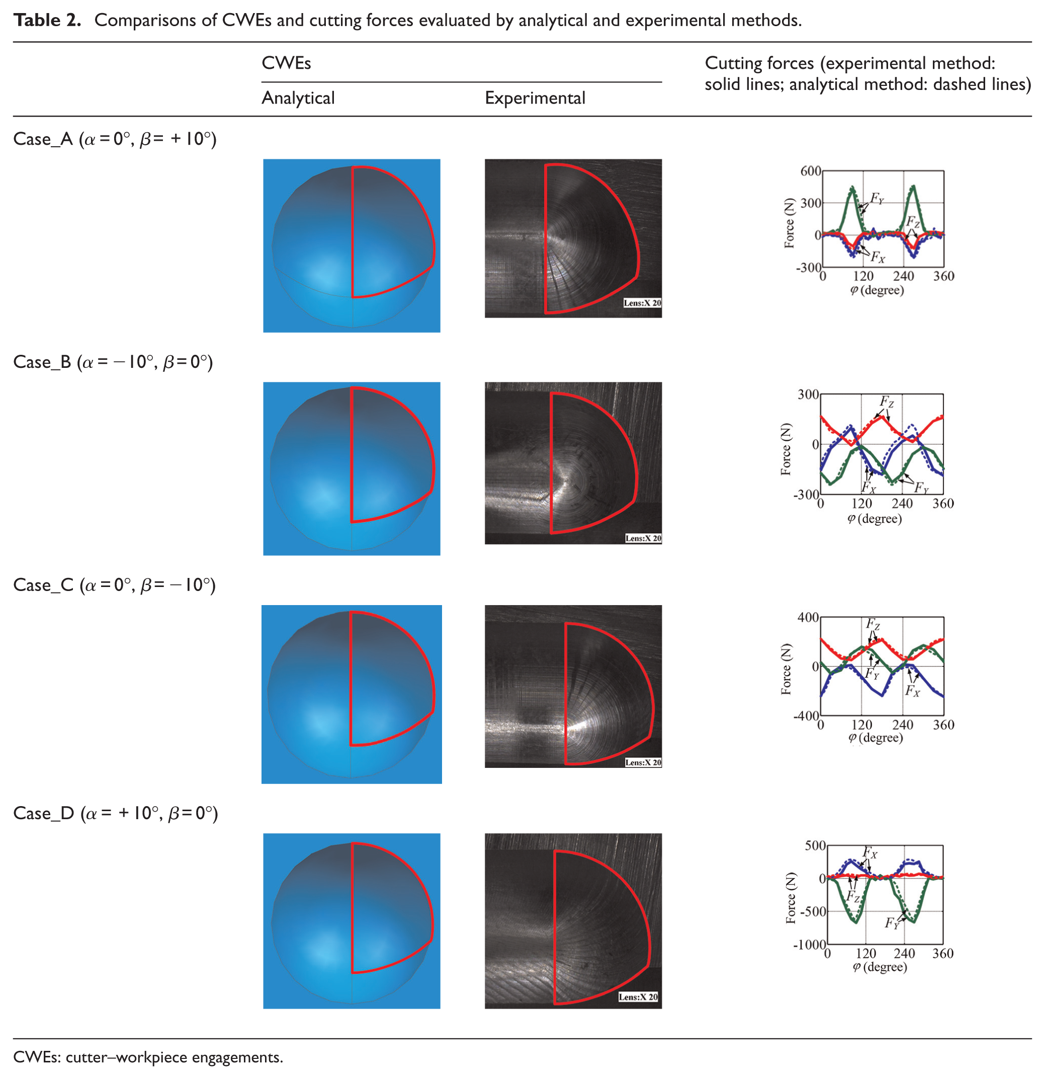
CWEs: cutter–workpiece engagements.
Table 2 shows the results (CWEs and cutting forces) obtained through analytical method presented here and experimental tests for four cases. Solid lines express the measured data, and dashed lines express the calculated data. These results with good agreement can verify the efficiency and accuracy of the model presented in this article.
Although only two examples are presented to illustrate the flexibility of the method proposed, the method can also be used for the arbitrary mills, which can be considered as revolution of an arbitrary section curve around the tool axis, resulting in a volumetric tool envelope. Noted that the arbitrary section curve is divided into lines and arcs, and equations (5), (6), (9), and (10) express the geometric relationships for each line and each arc. Equation (11) is used to evaluate the undeformed chip thickness, and equation (14) represents the element cutting forces.
Application in impeller machining
From the description in above section, there are three essential contents need to be cared to predict the cutting forces using the cutting force model presented previously, they are geometry of generalized milling, undeformed chip thickness, and cutting and edge force coefficients. The first one can be presented using generalized milling model, equations (4)–(9). The second one is evaluated using equations (10) and (11). And the last one can be determined using the mechanics of milling method. 26 CWE is identified using SAM presented in Ju et al. 38
To further illustrate the effectiveness of the model presented, a case study of an integrated impeller part milling using five-axis machine tool is an example to evaluate the cutting forces. The cutting experiment is performed on computer numerical control (CNC) machining center DMU-70V, the maximum spindle speed of which is 18,000 r/min, and the numerical control system of which is Heidenhain TNC 426. The machine tool have three translation axes (x, y, and z axes) which are achieved through spindle, and two rotating axes (b and c axes) which are achieved through worktable. Three solid carbide cutters corresponding to the HSK 63 Tool Holders are selected to perform the rough machining operation, semi-finish, and finish machining operations. The geometries of cutters used in experiments are listed in Table 3.
Cutter geometries used in experiments.
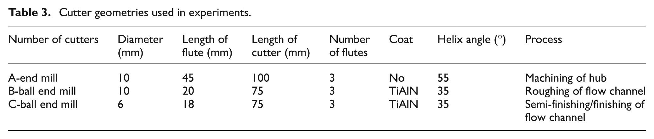
The cylinder workpiece with 130 mm of diameter is clamped on worktable through four-jaw chuck. The workpiece material is a 7050 aluminum alloy. Point and down milling operation is used from the middle to sides of flow channel. The impeller model has seven vanes and six flow channels. The bottom diameter of impeller is 130 mm, and the height is 62 mm. The minimum thickness of vane is 3 mm. The minimum space distance of flow channel is approximately 7.5 mm, and the maximum depth of vane is approximately 33 mm, so the overhang length of cutter needs to be larger than 33 mm. The surface of vane is of non-uniform rational b-spline (NURBS) shape. Therefore, the lead and tilt angles change obviously during cutting process. In this case, traditional cutting force model cannot be used to precisely catch and obtain instantaneous cutting force information. Simulated tool path is generated using the impeller module integrated in the commercial CAM software Hypermill®. The post-processing program is also transformed and inputted into CNC machining center through this module.
Take the rough machining process of one flow channel with B-ball end mill as an example, in which there are total 11-layer tool paths. The feed speed is 4000 mm/min, and spindle speed is 7000 r/min. The first-layer and fifth-layer tool path are analyzed here. The first-layer tool path contains 15-time cuttings, and the fifth-layer contains only 13-time cuttings due to the narrower space closing the bottom of impeller flow channel. To illustrate the effectiveness of the developed method, the first-, sixth-, and seventh-time cuttings of the first-layer tool path are chosen to predict the cutting force for the first cut case, which are indicated by 1-1, 1-6, and 1-7 as shown in Figure 6(a)–(c), respectively. And the first-, sixth- and seventh-time cuttings of the fifth-layer tool path are selected to explain the following cut case, which are indicated by 5-1, 5-6 and 5-7 as shown in Figure 6(d)–(f), respectively. It should be noted that for each cutting, both the lead and tilt angles vary with time. Additionally, there are 43 cutting position points for each cutting in the first-layer tool path, and 40 cutting position points for each cutting in the fifth-layer tool path, as show in Figure 6. With loss of generality, the 10th, 21st, and 32nd cutting position points for the first-layer tool path and the 10th, 20th, and 30th cutting position points for the fifth-layer tool path are selected to perform the further analysis. Therefore, total 18 cutting position points are analyzed here. It is obvious that only 1-1 and 5-1 are the first cutting cases, and 1-6, 1-7, 5-6, and 5-7 are the following cutting cases.
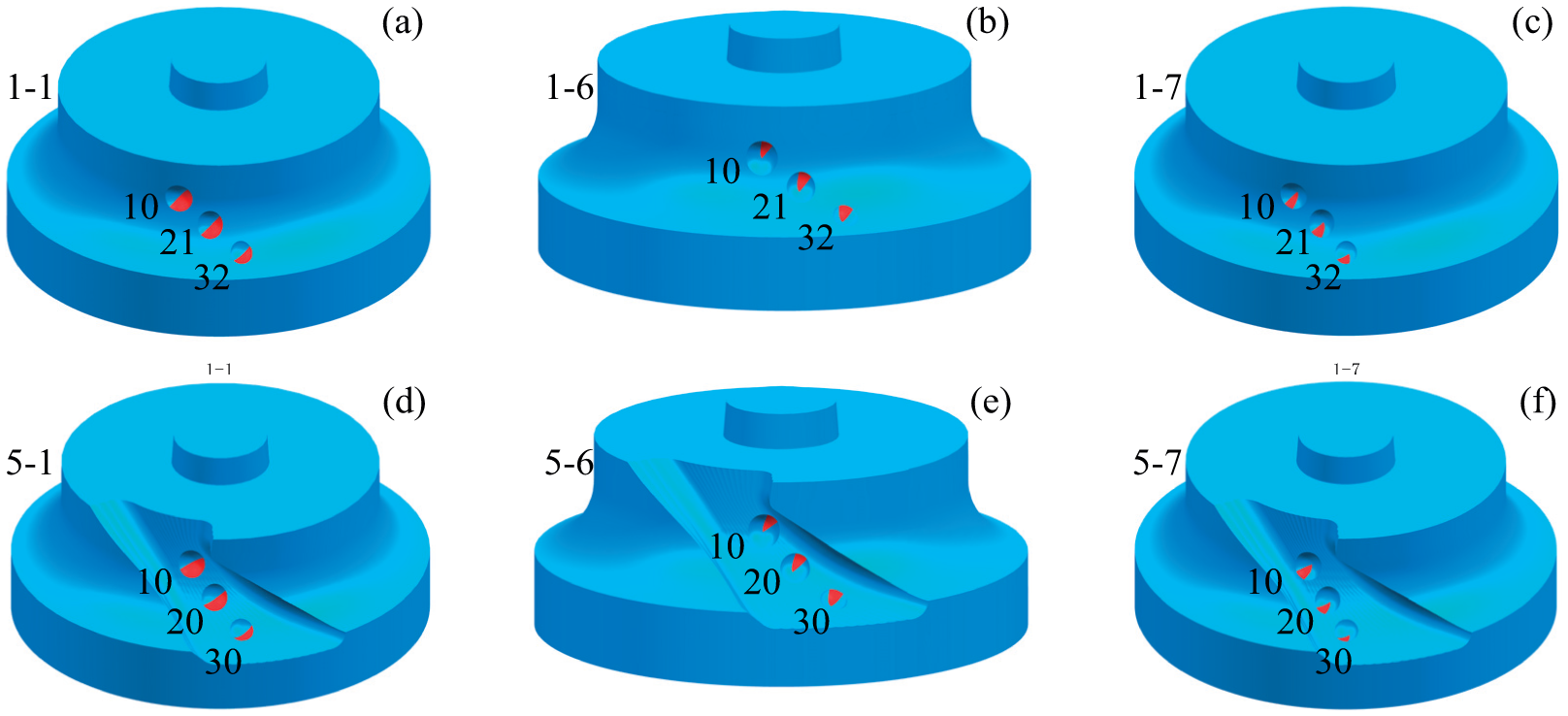
Eighteen cutting position points for two different layer tool paths; (a), (b) and (c): the first-, sixth-, and seventh-time cuttings of the first-layer tool path, respectively; (d), (e) and (f): the first-, sixth-, and seventh-time cuttings of the fifth-layer tool path, respectively.
Figure 7 shows the lead and tilt angles for six cutting processes (1-1, 1-6, 1-7, 5-1, 5-6, and 5-7). Blue dashed lines express the lead angles and red solid lines express the tilt angles. Figures (a)–(c) are the first-, sixth-, and seventh-time cutting for the first-layer tool path, respectively, and figures (d)–(f) are the first-, sixth-, and seventh-time cutting for the fifth-layer tool path, respectively. From Figure 7, it can be seen that in the third-time cuttings of the first-layer tool path, the lead and tilt angles are very close and approximate constants, which indicates that cutter forms simple space swept regions. Nevertheless, the lead and tilt angles have significant differences and change much for third-time cuttings for the fifth-layer tool path, which indicates the space swept regions of cutter is very complex. That is, the cutting forces for cases (a)–(c) can be predicted using literatures reported, while cannot do for cases (d)–(f).
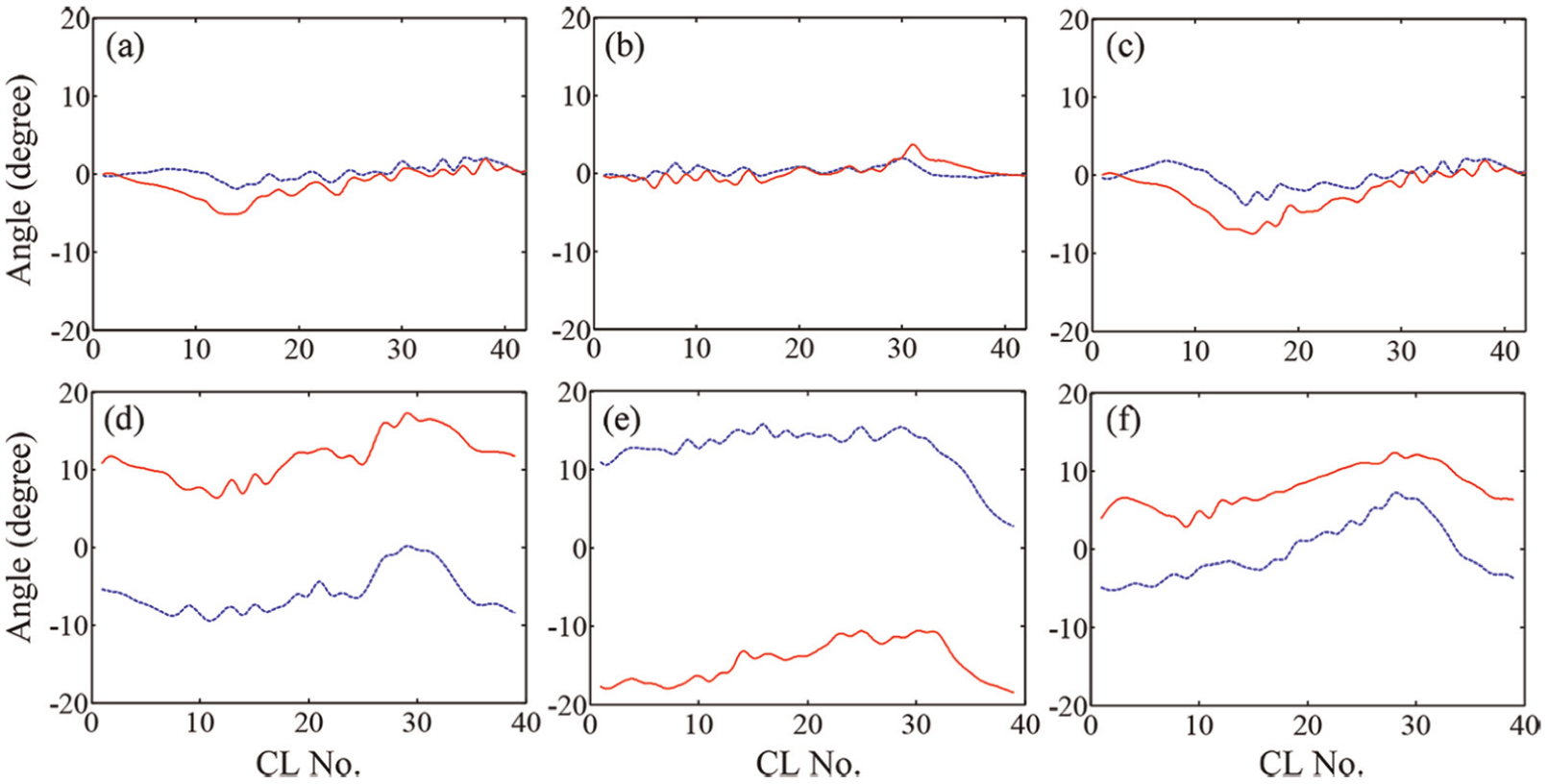
Lead (blue dashed lines) and tilt (red solid lines) angles for six cutting processes; (a), (b) and (c): the first-, sixth-, and seventh-time cuttings of the first-layer tool path, respectively; (d), (e) and (f): the first-, sixth-, and seventh-time cuttings of the fifth-layer tool path, respectively.
Figure 8 shows >the CWE information of nine cutting position points for the first-layer tool path, which is identified through SAM presented in Ju et al. 38 Figure 8(a)–(c) is the CWE data of the 10th, 21st, and 32nd position points for the first-time cutting (1-1), Figure 8(d)–(f) is the CWE data of the 10th, 21st, and 32nd position points for the sixth-time cutting (1-6), and Figure 8(g)–(i) is the CWE data of the 10th, 21st, and 32nd position points for the seventh-time cutting (1-7), respectively. It should be noted that here the nine cutting position points for the first-layer tool path are taken as an example, and the results for the fifth-layer tool path also can be obtained using the similar approach.
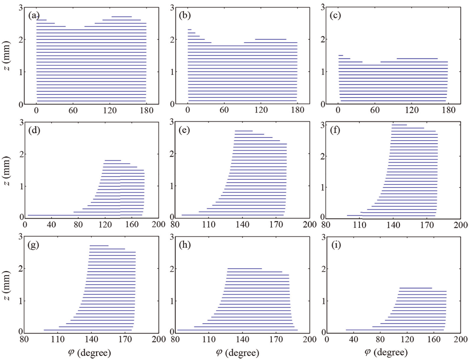
CWE information of nine cutting position points for the first-layer tool path; (a), (b) and (c): 10th, 21st and 32nd position points for the first-time cutting, respectively; (d), (e) and (f): 10th, 21st and 32nd position points for the sixth-time cutting, respectively; (g), (h) and (i): 10th, 21st and 32nd position points for the seventh-time cutting, respectively.
Similar with analysis presented in above section, substituting equations (26) and (28) into equation (11), the undeformed cutting thickness can be calculated. Corresponding to Figure 8, Figure 9 shows the undeformed chip thicknesses of 9 cutting position points for the first-layer tool path, which are evaluated through undeformed chip thickness model presented previously. The cases of diagrams (a)–(i) are the same with ones in Figure 8. It should be noted that all the information of CWEs and undeformed chip thicknesses are given in TCS coordinate frame in order to easily evaluate the cutting forces.
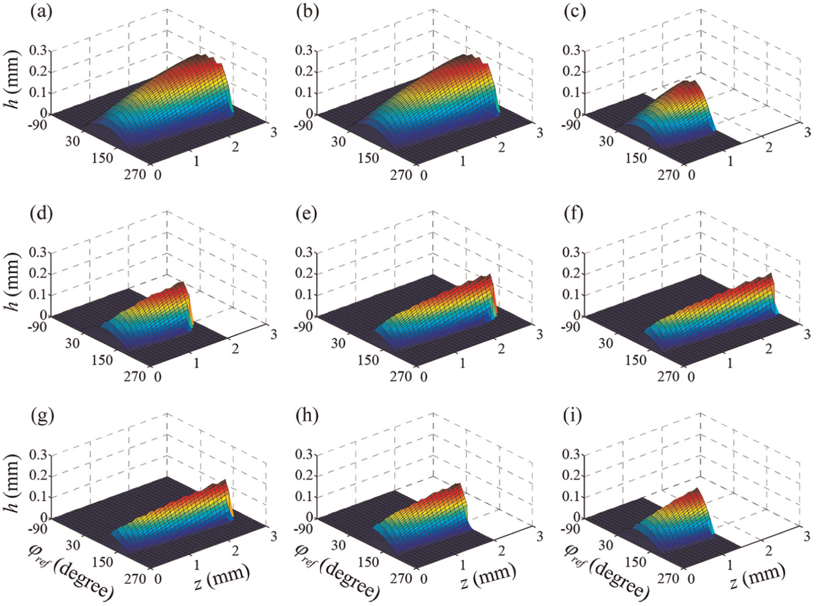
Undeformed chip thicknesses of nine cutting position points for the first-layer tool path; (a), (b) and (c): 10th, 21st and 32nd position points for the first-time cutting, respectively; (d), (e) and (f): 10th, 21st and 32nd position points for the sixth-time cutting, respectively; (g), (h) and (i): 10th, 21st and 32nd position points for the seventh-time cutting, respectively.
Figure 10 shows the instantaneous cutting forces of 9 cutting position points for the first-layer tool path, which are evaluated through equations (19) and (20). The cutting coefficients are as shown in Table 1.The solid lines indicate the cutting forces in GCS, and dashed lines indicate the cutting forces in TCS. And blue lines present the cutting force in x (X) direction, green lines present the cutting forces in y (Y) direction, and red lines present the cutting forces in z (Z) direction. The cases of figures (a)–(i) are also the same with ones in Figure 8.
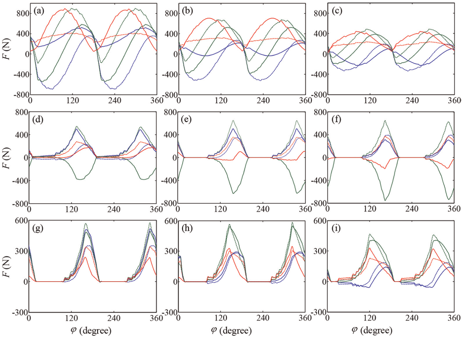
Instantaneous cutting forces of nine cutting position points for the first-layer tool path; (a), (b) and (c): 10th, 21st and 32nd position points for the first-time cutting, respectively; (d), (e) and (f): 10th, 21st and 32nd position points for the sixth-time cutting, respectively; (g), (h) and (i): 10th, 21st and 32nd position points for the seventh-time cutting, respectively.
From Figure 10, it can be seen that, first, the cutting forces change rapidly, which are dependent of tool path, cutter geometry, and cutting parameters. Second, for the same cutting cases (e.g. 1-1, Figure 10(a)–(c)), cutting forces in three cutting position points (10, 21, and 32) have the similar shape and oscillation period, except for different magnitudes. The reason is that lead and tilt angles do not change obviously, as shown in Figure 7. The advantage of the cutting force information is to be easy to predict and optimize the cutting process. Third, the cutting forces in the first-time cutting cases (1-1 and 5-1, figures (a)–(c)) are not zero in the whole one revolution of cutter (2π rad), which indicate that the cutter edges engage the workpiece in the one revolution. This is in agreement with the results of CWEs and undeformed cutting thickness, as shown in figures (a)–(c) in Figures 8 and 9. The cutting forces in the following cutting cases (1-6, 1-7, 5-6, and 5-7, figures (d)–(i)) are zero in some specific immersion angles in one revolution of cutter, which indicates that the cutter does not cutting workpiece at this time. These results are also consistent with those of CWEs and undeformed cutting thickness, as shown in figures (d)–(i) in Figures 8 and 9, respectively. Additionally, it can be found that there are differences between the cutting forces in GCS (in X, Y, and Z directions) and in TCS (in x, y, and z directions), especially for the 5-6 cutting case (Figure 10(d)–(f)), where the cutting forces are in the opposite directions. These results are dependent of two transform matrices used in equation (20),
It should be emphasized that the calculated cutting force results (as shown in Figure 10) represent the data at one fixed time point, and the experimental cutting force data are not measured in milling impeller process based the following reasons: (1) the CWEs identified and extracted using the SAM or other methods presented in the literatures published can only describe the instantaneous (at one fixed time point) engagement between cutter and workpiece for multi-axis milling (e.g. five-axis milling impeller). At the next time point, the CWEs vary, which is dependent of the cutter path. Therefore, cutting forces calculated based on the CWEs really represent the force information at that time point. If the overall force profile referring to one cutter path is required, all CWE data along to this cutter path are necessary. Obviously, it is impossible or impractical, or the amount of CWE data is very large. (2) Cutting forces are generally measured using the dynamometer (e.g. Kistler-type 9257B used in this article), which only permits the small sample piece being clamped. For the larger component, such as impeller, it is out of work. Certainly, there is another type of dynamometer, which can be fixed on the spindle of machine tool. In this case, the requirement for component is not necessary to be considered. However, for complex component, for example, impeller with relatively narrow flow channel, the interference between spindle-holder-tool with dynamometer and workpiece easily occurs, unless the longer cutter is used. Therefore, it is severely difficult to compare the cutting forces predicted with those measured for impeller five-axis milling. However, the method presented here can be verified through the simplified cutting tests, such as the multi-axis milling with constant tilt angles (section “Validation II: multi-axis milling with ball end mill”). This methodology is generally applied in many articles which focused on this item.
For multi-axis milling impeller, the rigidity of the blade is weaker and torsion resistance of the blade profile is very large. Thus, the thin-walled component milling, such as turbine blades and multi-frame monolithic components, is still a challenging problem due to the weak rigidity, time-varying modal parameter, and complex excitations (cutting forces). 41 Some articles have conducted the optimization of cutting parameters (optimal feed direction, 31 optimal cutter posture, 32 and tool path optimization33,34) for multi-axis milling process. And such generalized cutting force model knowledge presented in the article will help better understand and model multi-axis milling process, improving their machining stability and machining surface accuracy.
Conclusion
In this article, a generalized cutting force model for the fast and precise prediction of cutting forces with generalized milling cutter is presented. The developed model includes the generalized cutter geometry model, CWE model, and undeformed chip thickness model. The following conclusions can be summarized:
A generalized cutter geometry model is proposed through being regarded as a revolution of an arbitrary section curve composed of variable lines and curves around tool axis.
The undeformed chip thickness is calculated with respect to pre-defined TCS, which is transformed from FCN by lead and tilt angles.
A typical case study, rough machining process of aero-engine impeller is taken as an example to verify the availability of the model. In this case study, the CWE information, undeformed chip thickness, and cutting forces are evaluated in detail for 18 cutting position points in two-layer cutting process, which contains the two cutting cases (the first and the following cutting cases).
In the model presented, the tool path file and SAM are required to identify the CWE information. And it can be extended to an arbitrary generalized milling tool in multi-axis milling process as well as three-axis milling process and two-and-a-half-axis milling process.
Footnotes
Declaration of conflicting interests
The author(s) declared no potential conflicts of interest with respect to the research, authorship, and/or publication of this article.
Funding
The author(s) disclosed receipt of the following financial support for the research, authorship, and/or publication of this article: This work was supported by the National Natural Science Foundation of China (Grant No. 51575319), the Young Scholars Program of Shandong University (Grant No. 2015WLJH31), and Major National Science and Technology Project (Grant No. 2014ZX04012-014). This work was also supported by the Tai Shan Scholar Foundation (Grant No. TS20130922).