
Abstract
Electrolyte electrical conductivity plays a vital role as a process parameter during electrochemical macromachining as well as micromachining, especially during anode shape prediction and tool design. Electrolyte electrical conductivity during electrochemical machining varies due to generation of gas bubbles at the tool and workpiece surfaces, sludge due to the dissolution of workpiece material, and heat due to the flow of electric current in the circuit. The electrolyte becomes a multiphase system. A mathematical model to predict the electrolyte electrical conductivity in the multiphase system is presented in this article. An experimental study has also been carried out to validate the proposed model. This model has been applied to study the variation in electrolyte electrical conductivity along the electrolyte flow direction during electrochemical micromachining by measuring change in workpiece thickness. Optimum input machining parameters are also presented at which the change in electrolyte conductivity is negligible in the machining zone.
Introduction
Electrochemical machining (ECM) is an advanced machining process (AMP) for electrically conducting materials. It has many advantages over other AMPs such as higher material removal rate (MRR), no recast layer, and no thermal residual stresses. ECM process works on the principle of anodic (workpiece) dissolution, and its machining performance is independent of workpiece hardness. The machining accuracy and precision can be controlled by various process parameters such as voltage, feed rate, inter-electrode gap (IEG), and type and concentration of electrolyte. 1 Electrolyte electrical conductivity plays an important role in macro- and microscale ECM in general 2 and during anode (workpiece) shape prediction and tool (cathode) design in particular 3 (now onwards, both electrochemical (EC) micromachining and EC macromachining are included in the term ECM for this article). However, electrolyte electrical conductivity (now onwards, named as electrolyte conductivity) during ECM varies along the electrolyte flow direction in the machining zone due to various reactions taking place in the system, for example, sludge formation due to workpiece dissolution, generation of gas bubbles at tool and workpiece surface due to chemical reactions, and change in electrolyte temperature due to heat generation. Hence, it is important to study the change taking place in the electrolyte conductivity in the machining zone which in turn affects the machining accuracy and performance of the process as a whole.
There have been many studies to understand the effect of different phases (liquid, solid, gas) in a continuum on the electrical conductivity of the system. Maxwell 4 proposed a model for low-concentration dispersions of uniform spheres
where
Rayleigh’s 5 model assumed uniform sized spheres arranged in a simple cubic array and Weiner’s 6 model considered very low concentration of spherical dispersion. But Meredith and Tobias 7 considered dispersions of uniform spheres arranged in cubic lattice for their model of electrolyte conductivity. Yianatos et al. 8 proposed a model for non-conductive dispersed phase, one for dilute phase and another for high-concentration phase. Bruggeman 9 extended Maxwell’s 4 model for large-sized spheres of dispersion phase
Weissberg’s 10 model considered dispersion of uniform as well as non-uniform spheres, while a model considering spheroid shaped dispersion was proposed by Fricke. 11
In real life, many times one may not have regular shaped dispersion, hence De la Rue and Tobias 12 proposed an empirical expression for irregular shaped dispersions. Prager’s 13 model was based on generalized diffusion, for a suspension of solid particles, in terms of statistical parameters for a random geometry. In Böttchers 14 model, dispersion system was assumed to be a close mixture of two kinds of spherical particles disperse phase and dispersion medium. Achwal and Stepanek 15 proposed an empirical model using 6-mm Raschig rings and 6-mm ceramic cylinders. Beaovich and Watson’s 16 model was developed using 4- to 6-mm alumina and Plexiglass beads. Kato et al. 17 worked on 0.4 to 2.2-mm glass beads for their model.
To consider the effect of gas phase and temperature, Hopenfeld and Cole 18 and Thorpe and Zerkle 19 independently proposed the following equation

where
Thus, there have been various models for electrical conductivity in three phase dispersions. However, there has been no study which has either used the above-developed models or proposed a new model(s), to study the effect of volume fraction of sludge and gas, as well as temperature (all varying at the same time) on the electrolyte conductivity during ECM (both as macro- and microlevel). The variation of electrolyte conductivity in micromachining and microtexturing plays an important role.20,21 Electrolyte conductivity variation is important not only in ECM and electrochemical micromachining (ECMM) but also in hybrid ECM and ECMM processes, namely, ultrasonically assisted EC micro drilling and travelling wire EC spark machining. If electrolyte conductivity cannot be evaluated accurately, then the predicted optimum machining conditions will not give the desired results.22–24
Mathematical modelling
During ECM, as the electrolyte flows from the inlet towards the outlet, rise in the temperature of electrolyte (due to current flow in the circuit), evolution of hydrogen gas bubbles at cathode and oxygen gas bubbles at anode, and sludge formation at anode start taking place in machining zone. 1 To evaluate accurate IEG in the machining zone, knowledge of electrolyte conductivity is a pre-requisite. This article deals with the evaluation of effective electrolyte conductivity along the electrolyte flow direction during ECM. Hence, to understand the effect of variation in different input parameters on the electrolyte conductivity during ECM, a mathematical model is developed. Furthermore, a comprehensive empirical relationship is also proposed to predict the electrolyte conductivity with varying volume fraction of sludge and bubbles and varying temperature in the machining zone.
Modelling of electrolyte conductivity in multiphase system
For modelling electrolyte conductivity, Maxwell’s 4 and Bruggeman’s 9 models are extended to multiphase system with the following assumptions:
The solution is dilute enough such that the presence of one dispersed phase does not affect the electric field around the other one.
The shape of the dispersed phase is spherical and very small in size.
Electric field is uniform throughout the space.
Laplace’s equation in spherical co-ordinate system can be written as follows
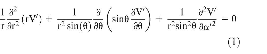
where V′ is the electric potential, r is the distance of a point from the origin, α′ is the angle of the projection of the line joining origin and point on X–Y plane with x-axis, and
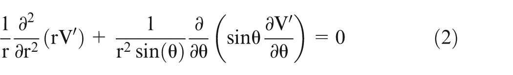
For a potential field with Azimuthal symmetry (i.e. rotational symmetry) about the z-axis, V′ does not vary with α′. Hence,
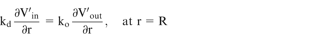
On applying the boundary conditions for a sphere of radius R, the following conditions are obtained:
The potential at the surface of the sphere calculated from

No surface charge is present on the surface, hence
The electric field at a distance

On solving equation (2) and considering ‘n’ number of spheres, the potential can be given by
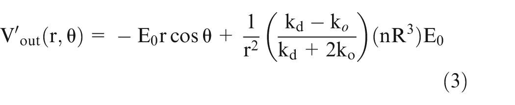
where
On extending this model to multiphase system based on the same approach as in Maxwell equation given above and considering
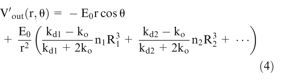
Consider a large sphere containing medium with radius ‘y’ and conductivity
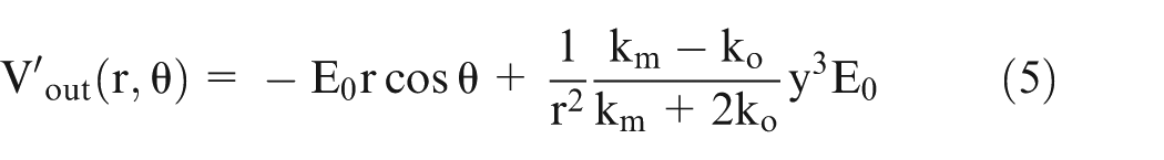
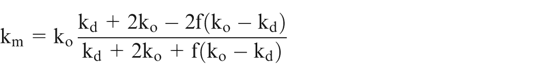
Equate equation (4) with equation (5) and simplify it to obtain the following equation
Here,
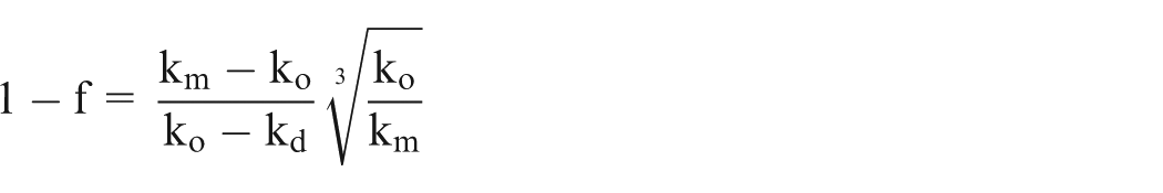
In Bruggeman’s approach 9 for random dispersion of spherical particles with a wide range of size, it is assumed that if a relatively larger particle is added to the solution which already has much smaller particles, then the disturbance due to the presence of smaller particles will be negligible
Similarly,
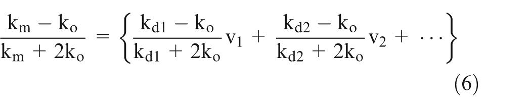
where
It can also be written as
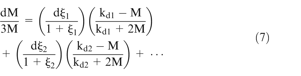
At
Equation (7) can be used in case of alloy as workpiece material because various constituent materials of the alloy form different types of sludge during anodic dissolution. Although the equation is derived in spherical co-ordinate system, it can be used for any shape of the system provided the shape of the dispersed particle is spherical. In this work, pure metal is used as workpiece, hence bubbles and only one kind of sludge will be produced.
The electrical conductivity of gases can be taken as zero for the voltages used in ECM process. The type of sludge depends on the workpiece material used. The electrical conductivity of sludge particles is very small as compared to the electrical conductivity of electrolyte. This equation can be numerically solved by many methods; however, in this work, Ranga–Kutta method is used to solve it.
It is found 25 that the effective conductivity of electrolyte is decreasing almost linearly with an increase in the sludge volume fraction and bubble’s volume fraction. However, if the sludge formed is electrically conductive, then the effective conductivity of the electrolyte would increase with an increase in sludge volume fraction provided bubble’s volume fraction remains constant.
Assuming that the relationship of variation in electrical conductivity with temperature is very well established, the following generalized equation (8) is proposed to evaluate effective conductivity accounting for temperature, gas void fraction, and sludge volume fraction
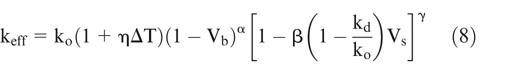
where
η, α, β, and γ in equation (8) can also be evaluated from the pilot experiments for specific cases. This equation is equally applicable for EC macromachining as well as EC micromachining. However, the numerical values of changes in ΔT, Vb, and Vs in case of EC micromachining are likely to be different from those in EC macromachining. 25
Electrolyte conductivity variation
Consider the schematic diagram (Figure 1) of the setup for ECM. Both tool and workpiece are assumed to be planer in geometry. Following assumptions are made while deriving the relationship for electrolyte conductivity:
Hydrogen gas bubbles produced during ECM behave as the ideal gas.
Oxygen gas production is assumed to be too small for realistic consideration.
Initially, IEG is assumed to be same everywhere along the electrolyte flow direction.
Ohm’s law is followed in the IEG during ECM.
Volume change of gas due to temperature change during ECM is negligible.
Heat capacity and temperature coefficient of electrolyte do not vary significantly due to the presence of bubbles and sludge.
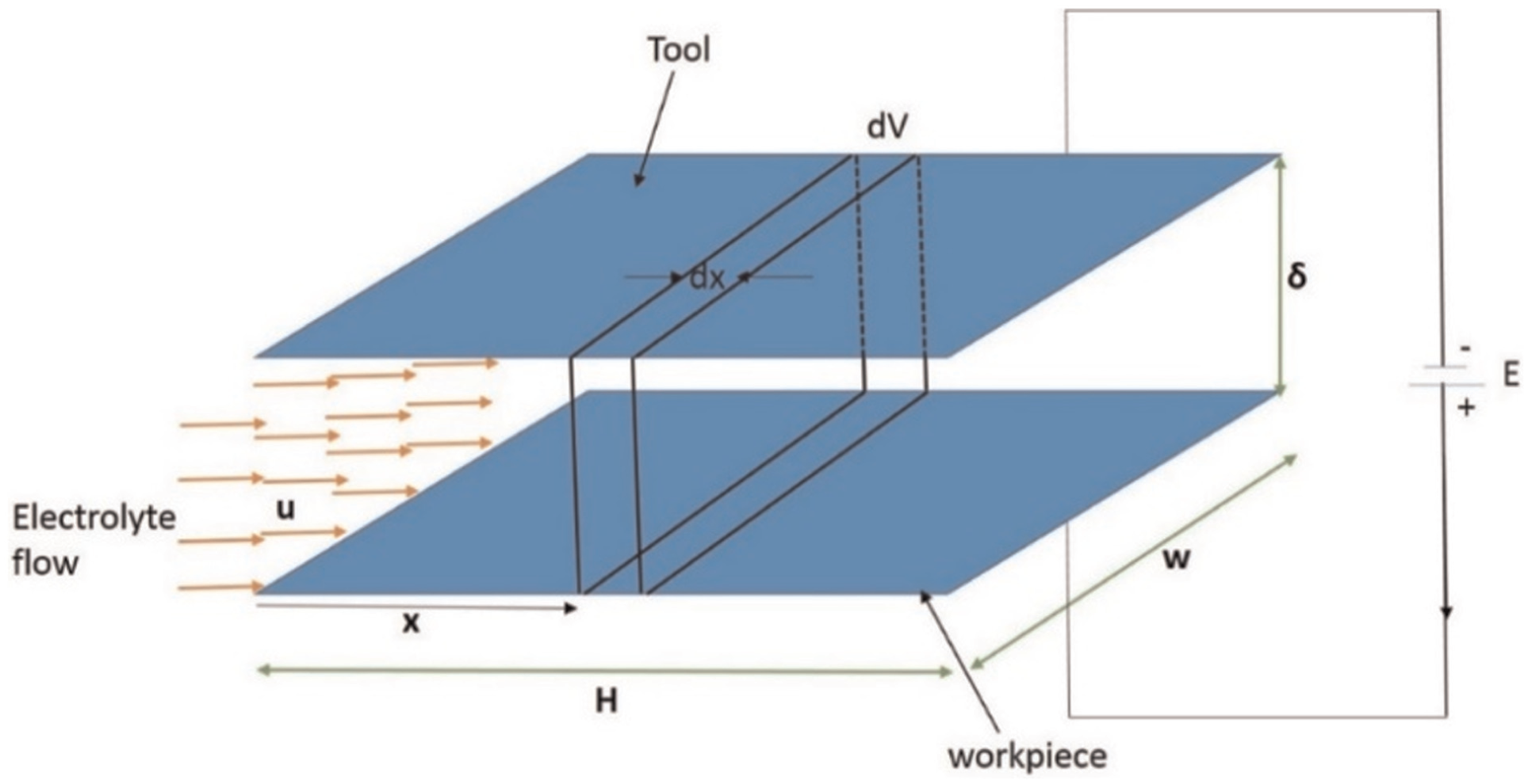
Schematic diagram of electrochemical machining.
In acidic medium, hydrogen gas is evolved at the cathode. Using ideal gas equation and Faraday’s laws of electrolysis, it can be written as
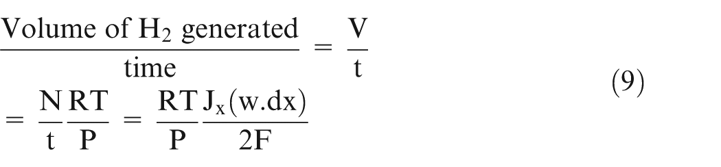
where P is the pressure, V is the volume, N is the number of moles, R is the gas constant, T is the temperature, w is the width of the workpiece, t is the machining time, and F is Faraday’s constant.
Equation (9) gives the volume of gas added in the volume ‘dV’ as shown in Figure 1. The gas exiting the volume ‘dV’ is more than the gas volume entering because there is gas generation in this small volume ‘dV’ due to chemical reaction at anode and cathode. It can also be written as
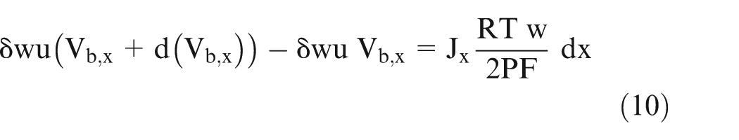
where
Here, the term on the left hand side (LHS) represents the difference between the volume of exiting gas and the entering gas, and the right hand side (RHS) represents the volume of the gas generated in volume ‘dV’.
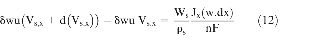
At the anode, sludge is generated as follows and it can be written as equation (11)
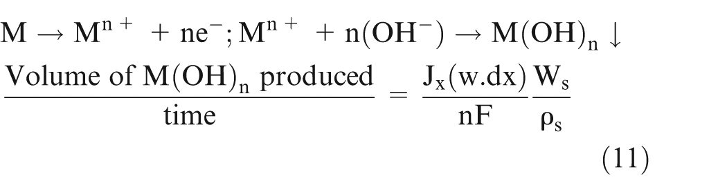
where
Equation (11) gives the volume of sludge added in the volume ‘dV’ (Figure 1). It can also be written as mass conservation equation. Here, the term on the LHS represents the difference between the amount of sludge exiting and entering the volume ‘dV’, and the RHS represents the volume of sludge generated in volume ‘dV’
where
Neglecting the effect of temperature (in above expression,
If ‘E’ is the potential difference across the electrodes, then using Ohm’s law and putting the value of
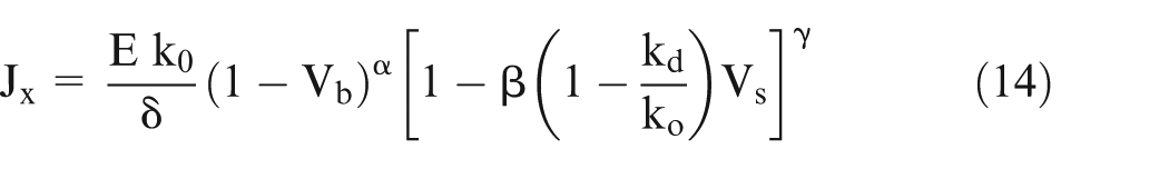
Putting the value of
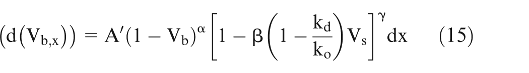
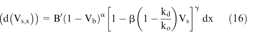
where
Thus, the values of A′ and B′ can be calculated from the values of input process parameters.
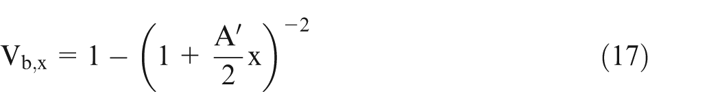
Equations (15) and (16) can be solved numerically by varying x from 0 to x,
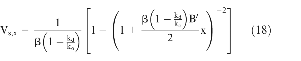
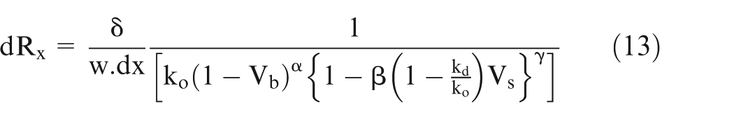
The effective conductivity of electrolyte can be calculated using parallel resistance approach. In this approach, the resistance of small volume is calculated and then taking them as parallel resistances, the total resistance has been calculated.1,3 The resistance of the small volumes is calculated using equation (13). Now, the effective conductivity is calculated as follows.
Equation (13) gives the value of
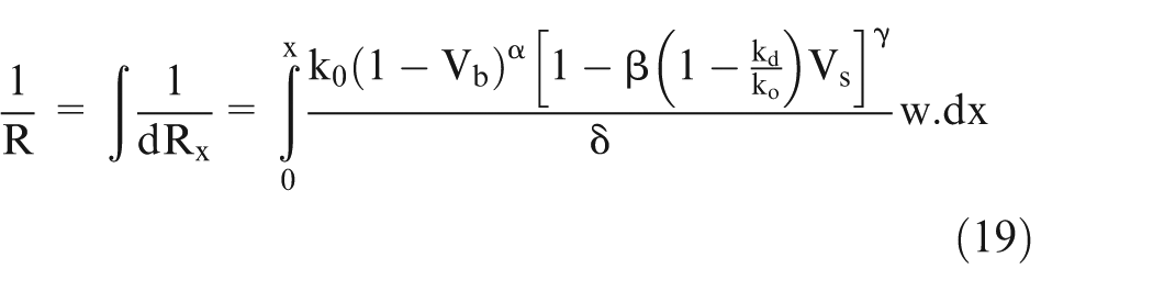
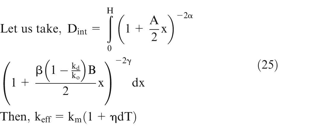
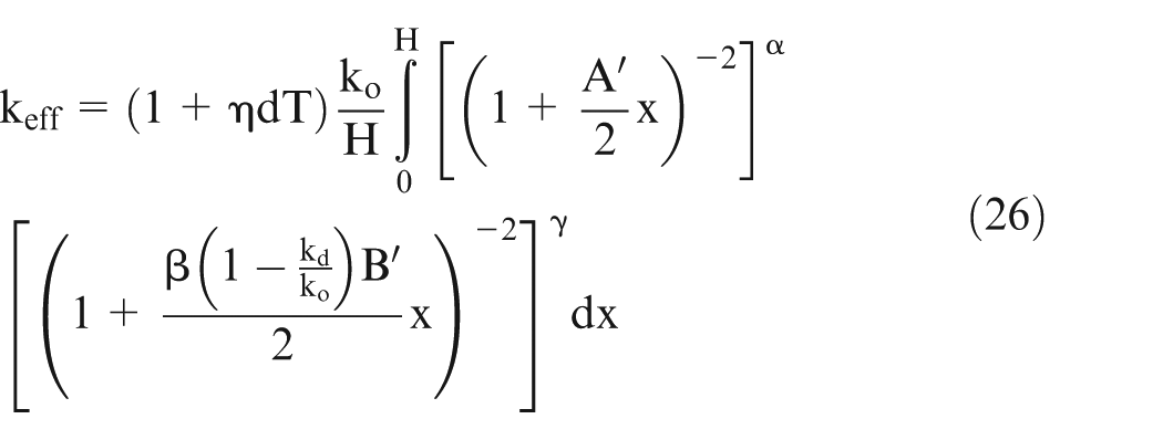
Let effective conductivity be ‘km’ and H be the length of the workpiece, then it can be shown 25 that
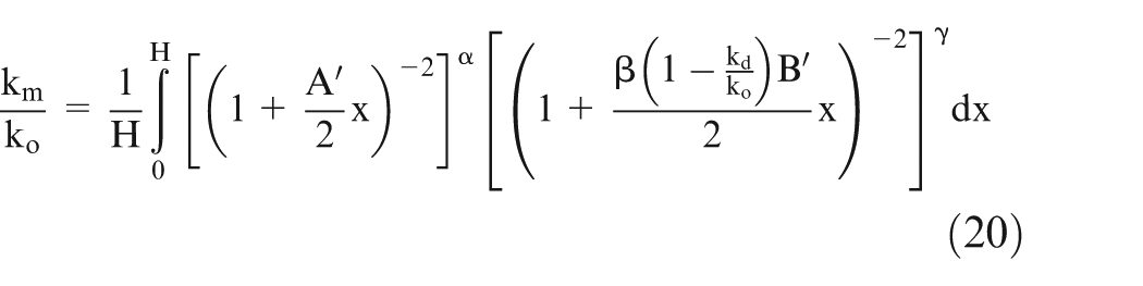
Assume
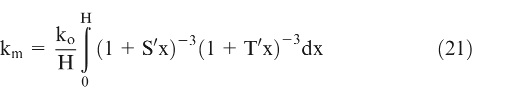
Equation (21) can be solved numerically using the values of
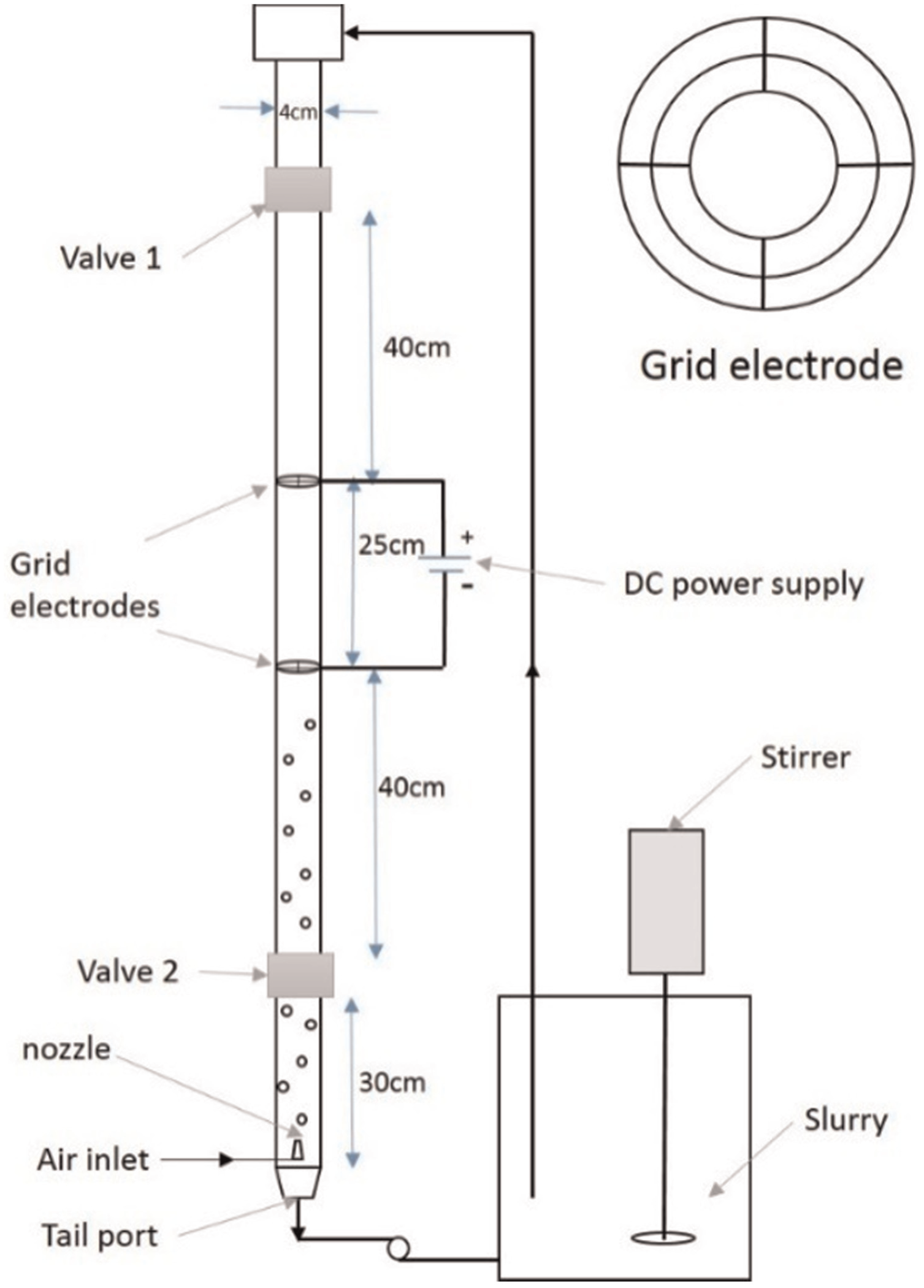
Schematic diagram of the experimental setup for multiphase conductivity measurement.
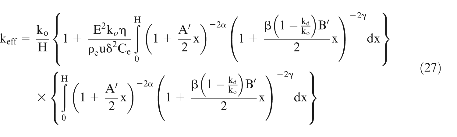
Heat generated in the volume
Using above equations and Ohm’s law, it can be shown
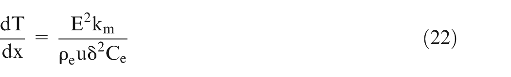
Putting the value of ‘km’ in equation (22) and simplification will give
It is known that the electrical conductivity is directly proportional to
where ‘km’ represents the electrical conductivity of electrolyte which includes the effect of gas bubbles and sludge.
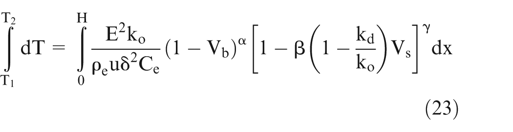
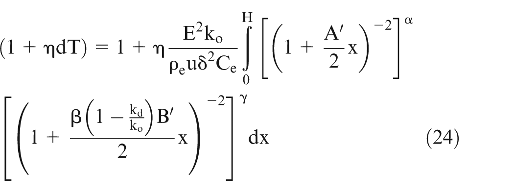
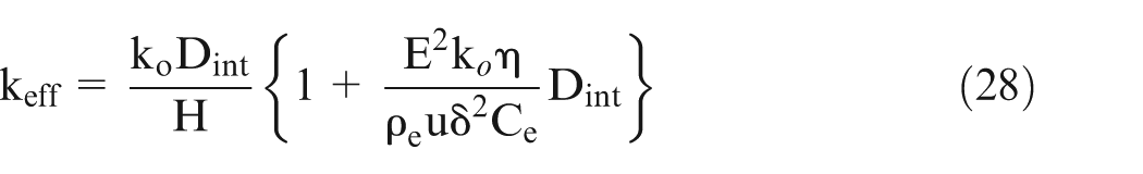
Using above derivations, it can be shown
Substitute the value of
Model validation experiments
The conductivity changes along the electrolyte flow direction but it is difficult to calculate. Hence, an indirect methodology is used to verify the proposed mathematical model. The thickness change (Figure 1) is directly related to the effective electrolyte conductivity (equation (28)), hence a change in electrolyte conductivity is correlated to the change in thickness at different points along the x-axis. Thus, the electrolyte conductivity change can be indirectly experimentally verified.
Considering zero feed rate of the tool, the linear MRR (MRRl) is given 1 by equation (29)
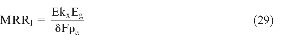
where
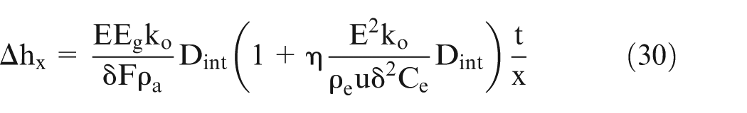
Substituting the value of kx and multiplying MRRl by machining time t”, it can be shown
Experimental setup and procedure
Two sets of experiments were conducted to validate the proposed electrolyte conductivity model. Figure 2 shows a setup used to measure electrolyte conductivity in a multiphase system. ‘Isolating technique’ was used to measure the conductivity of the electrolyte. 8 A column of 4-cm diameter and 150-cm height with two valves was used to enclose a section where the electrolyte conductivity was measured. The dimensions of the valves were chosen in such a way that the inner diameters of the valves and column were equal in order to minimize the disturbance in the hydrodynamics of the system. The electrodes made of copper in the grid form (Figure 2) were used to measure the conductivity and to minimize the disturbance to the flow. Very fine needles (diameter = 100 μm) were used as nozzle connected to the compressed air supply. The volume flow rate was monitored by the pressure gauge connected to the supply line.
During the experiments, solid phase (SiC or Alumina powder) was mixed with the electrolyte and glycerol, and it was well stirred. Glycerol was used as a frothing agent to reduce surface tension of the slurry in order to stabilize the bubbles formed. The slurry formed was then pumped to the uppermost point in the column, and it was allowed to flow by gravity inside the column. Over flow was avoided by controlling flow rate of the slurry, ensuring that whole liquid would eventually leave through the tail port and back to the container for recirculation. The gas flow was controlled by a knob operated valve which was connected to a compressed air supply system. The system was allowed to remain in this position for some time in order to achieve a steady state flow. Five different locations were marked along the length of the workpiece using a ‘co-ordinate measuring machine’ (CMM) where its thickness was measured.
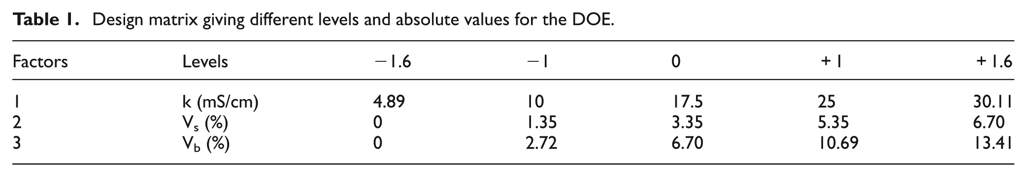
Direct current (DC) voltage was applied across the electrodes, and voltage and current readings were recorded. The voltage was kept low to achieve low current density at the electrodes in order to avoid polarization effect. When the current reading stabilized, both the valves were closed simultaneously, thus isolating three-phase samples from the rest of the system. The volume fraction of gas phase was obtained by measuring volume of air accumulated in the upper section of the column below valve1 and dividing it by the total volume (1350 mL) assuming that it is uniformly distributed. Central composite design was used to plan the experiments. Table 1 shows various levels of different factors and their absolute values. In this table, k is electrolyte conductivity. Vs and Vb are volume fraction of sludge and bubbles, respectively.
Design matrix giving different levels and absolute values for the DOE.
The second set of experiments was aimed to study the thickness reduction in the workpiece along the electrolyte flow direction during ECM. In this work, Hyper 10 (Multi Process Micro Machine Tool supplied by Sinergy Nano Systems, India) was used to carry out ECM experiments. The experimental setup involves flat workpiece and flat copper tool (Figure 1) in order to keep the electrolyte flow laminar and maintain a uniform IEG.
Containment was designed to make the flow of the electrolyte strictly in the IEG. Electrolyte velocity was controlled by the valve attached to the electrolyte flow pipe. Prior to the experiments, the thickness of the workpiece and tool were measured at five different points. At the start of the experiment, IEG = 1 mm was maintained using a computer numeric control (CNC) machine. Temperature of the electrolyte and its electrical conductivity at the inlet were recorded. Each experiment was conducted for a certain period of time. After the experiment was over, the workpiece was taken out and the thickness was again measured at the same five marked positions using the CMM. The change in the thickness was calculated for further analysis.
Results and discussions
Effect of temperature, void fraction, and sludge on the electrolyte conductivity using the proposed model has been studied. Furthermore, the experimental results have been compared with the results obtained from the proposed model for electrolyte conductivity.
Effect of temperature on the electrolyte conductivity
The variation of electrolyte conductivity with temperature has been well studied; however, it has been studied again in this work to give more credibility to the developed model. By plotting
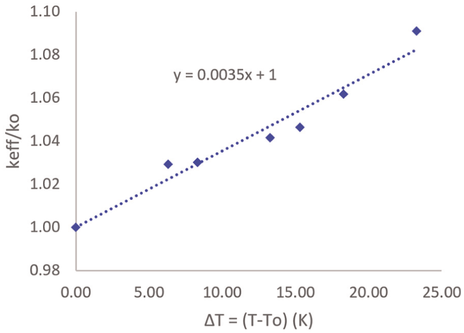
Variation of electrolyte conductivity ratio with temperature.
Effect of solid and gas phases on the electrolyte conductivity
In these experiments, pure electrolyte was pumped into the column. The conductivity of pure electrolyte at different concentrations was measured at different values of bubbles volume fraction. Theoretical value of conductivity was calculated using this equation
Thus, the electrical conductivity decreases with an increase in both the volume fractions of gas bubbles and the sludge. The variation in the experimental results does not fully coincide with the variation in the model results. This deviation varies from 0.02% to 2.99%. There can be various reasons for this. These experiments were conducted when only one parameter was varied at a time. The model assumes very small bubble’s size such that it does not disturb the electric field after a certain distance. However, during the experiments, the bubble’s size was much larger (in mm range) at high pressure. This could have led to more reduction in the electrolyte conductivity than the values predicted by the model. 25
The experiments were designed using central composite design by varying both bubble volume fraction and sludge volume fraction. From the experimental results, following polynomial equation for the effective electrolyte conductivity was obtained
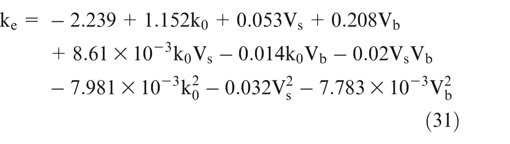
Experimental results in Figs 4 & 5 have been calculated using Eq. (31), which is derived from the experimental data. Theoretical results are evaluated using numeric solutions of Eq. (28). Figure 4(a) shows the variation of electrolyte conductivity with volume fraction of bubbles for different volume fractions of sludge contents. The conductivity value decreases with an increase in volume fraction of bubbles. The electrolyte conductivity further decreases as the sludge fraction is increased for a particular value of volume fraction of bubbles (Figure 4(a)). The reduction observed was considerable. For an increase in volume fraction of sludge for 2%, 5%, and 7% for volume fraction of bubbles at 20%, the reduction in electrolyte conductivity was 30.48%, 45.26%, and 57.97%, respectively, compared to the k value at 0% volume fraction of bubbles.
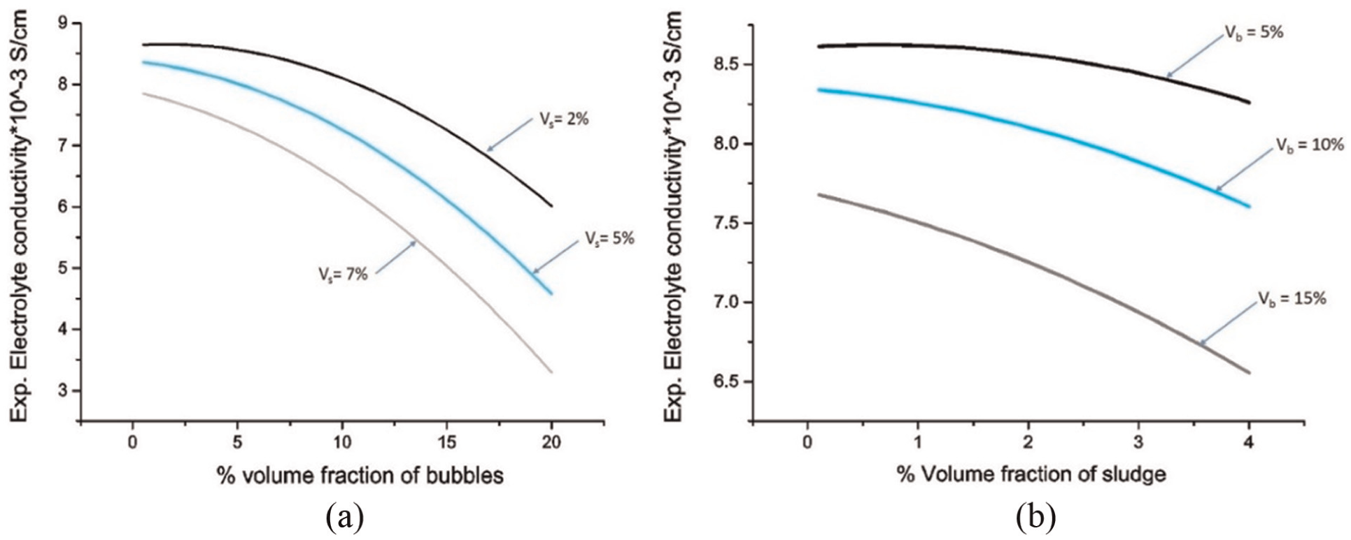
(a) Variation of electrolyte conductivity with bubbles percent volume fraction and (b) variation of electrolyte conductivity with sludge percent volume fraction.
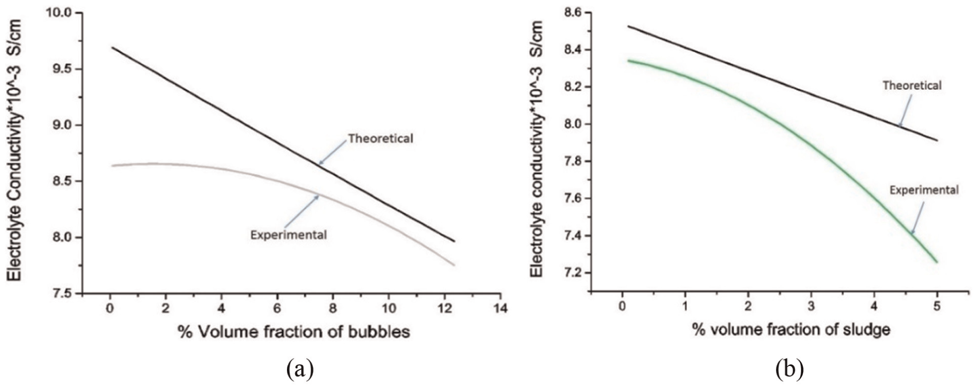
Relationship between conductivity values obtained from experimental model and theoretical values for varying volume fraction of (a) bubbles and (b) sludge.
Figure 4(b) shows the change in electrolyte conductivity with volume fraction of sludge for different values of volume fraction of bubbles. The conductivity of electrolyte decreases with an increase in sludge volume fraction. The volume fraction of solid particles varied from 0% to 4% for different volume fractions of bubbles (5%, 10%, and 15%).
The experimental and theoretical values of electrolyte conductivity are compared in Figure 5(a) and (b). Although, the electrolyte conductivity decreases both in theoretical model prediction and in experimental results. However, the experimental values of electrolyte conductivity deviate from the theoretical values. In Figure 5(a), the experimental values deviate from 2.67% to 10.84% of theoretical values of electrolyte conductivity. Figure 5(b) compares the experimental and theoretical values of electrolyte conductivity versus solid phase (sludge) content. The deviation in the two values ranges from 2.17% to 8.29%. There can be several reasons for this deviation. The bubble’s size was taken to be very small while developing the model; however, during the experiments, the bubble’s size was relatively high. The details have already been discussed in the preceding section. The electrode polarization during experimentation might be another reason for higher reduction in electrolyte conductivity than the expected one. The polarization of electrodes was minimized by having very low current density. The deviation of the experimental values was within 10.26%. Hence, the model developed can be considered in reasonably good agreement with the experimental results.
Reduction in the workpiece thickness during ECM
The electrolyte conductivity varies along the electrolyte flow direction in ECM. A change in the electrolyte conductivity due to a change in temperature, % concentration of bubbles and % concentration of sludge particles, changes IEG. In other words, for this case, it changes linear MRR. Hence, a change in thickness of the workpiece (Δh) along the electrolyte flow direction takes place. Figure 6(a) compares theoretically predicted Δh with the experimental values of Δh along the electrolyte flow direction. Table 2 shows the values of the initial input parameters. The value of electrolyte conductivity was chosen very low in order to make the effects of gas bubbles, sludge particles, and heat more visible.
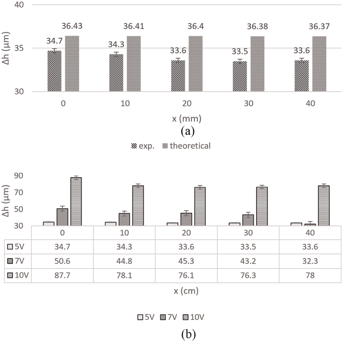
(a) Comparison between experimental and theoretical values of reduction in thickness of workpiece at 5 V along the electrolyte flow direction and (b) experimental values of reduction in thickness of workpiece along electrolyte flow direction at different voltages.
Values of input parameters.
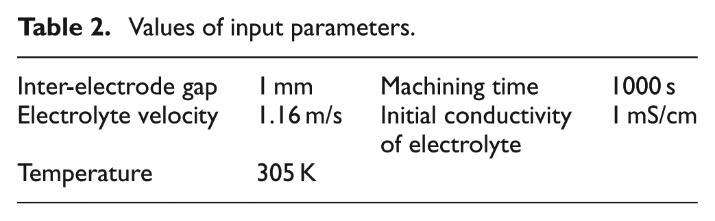
Figure 6(b) compares the reduction in thickness of the workpiece experimentally observed and theoretically calculated for different applied voltages. In general, the change in thickness value (Δh) decreases along the electrolyte flow direction. In other words, the thickness of the workpiece increases along the electrolyte flow direction, implying that the material removal is maximum at the electrolyte inlet point and minimum at the electrolyte exit point. Linear MRR is directly proportional to the electrolyte conductivity (equation (29)), and it is decreasing along the electrolyte flow direction. However, there has been some difference between the theoretically predicted value and the experimental observations. There can be several reasons for the deviation. The flow of electrolyte is assumed to be laminar, but during the experiments there might be some turbulence, which could in turn affect the sludge and bubbles distribution in the electrolyte. As mentioned earlier, several heat sources generating heat and absorbing heat were also neglected. Furthermore, the theoretical values are greater than the experimental values (Figure 6). The reason for this could be inefficient flushing of sludge. During the experiments, the sludge was not fully flushed out due to large length of the workpiece (50 mm) and relatively low electrolyte velocity. This would mean accumulation of reaction products (dissolved metal) on the workpiece surface, which in turn could have prevented further machining, thus resulting in lower values of thickness change than the predicted ones.
Constant electrolyte conductivity in the machining zone during ECM
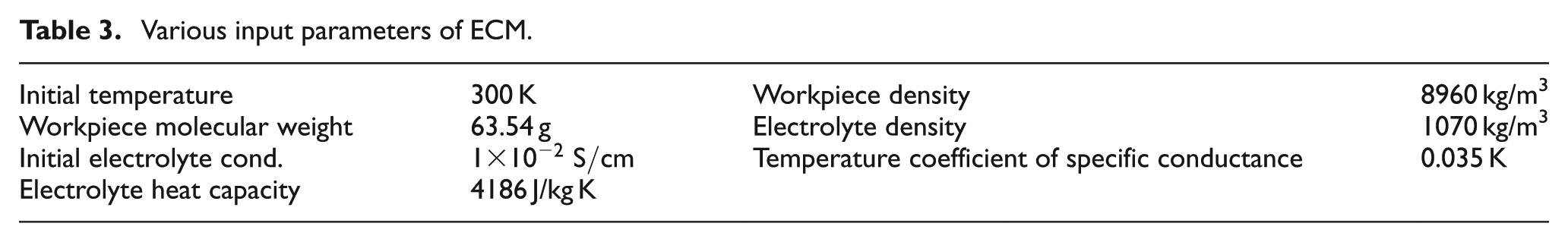
It is found 25 that the electrolyte conductivity does not vary much along the electrolyte flow direction if the IEG and electrolyte flow velocity are kept high, definitely at the cost of low MRR. However, in case of voltage, the value lies between 10 and 15 V where the effect of sludge and bubbles on electrolyte conductivity is equal and opposite to that of heat generation. The cumulative effect of heat, sludge, and bubbles is also shown in Figure 7. Now, the question arises: whether it is possible to have the machining conditions at which the electrolyte conductivity remains almost constant throughout the machining zone during ECM? Some numerical experiments were conducted (input parameters (Table 3)) for which the results are discussed in the following paragraphs.
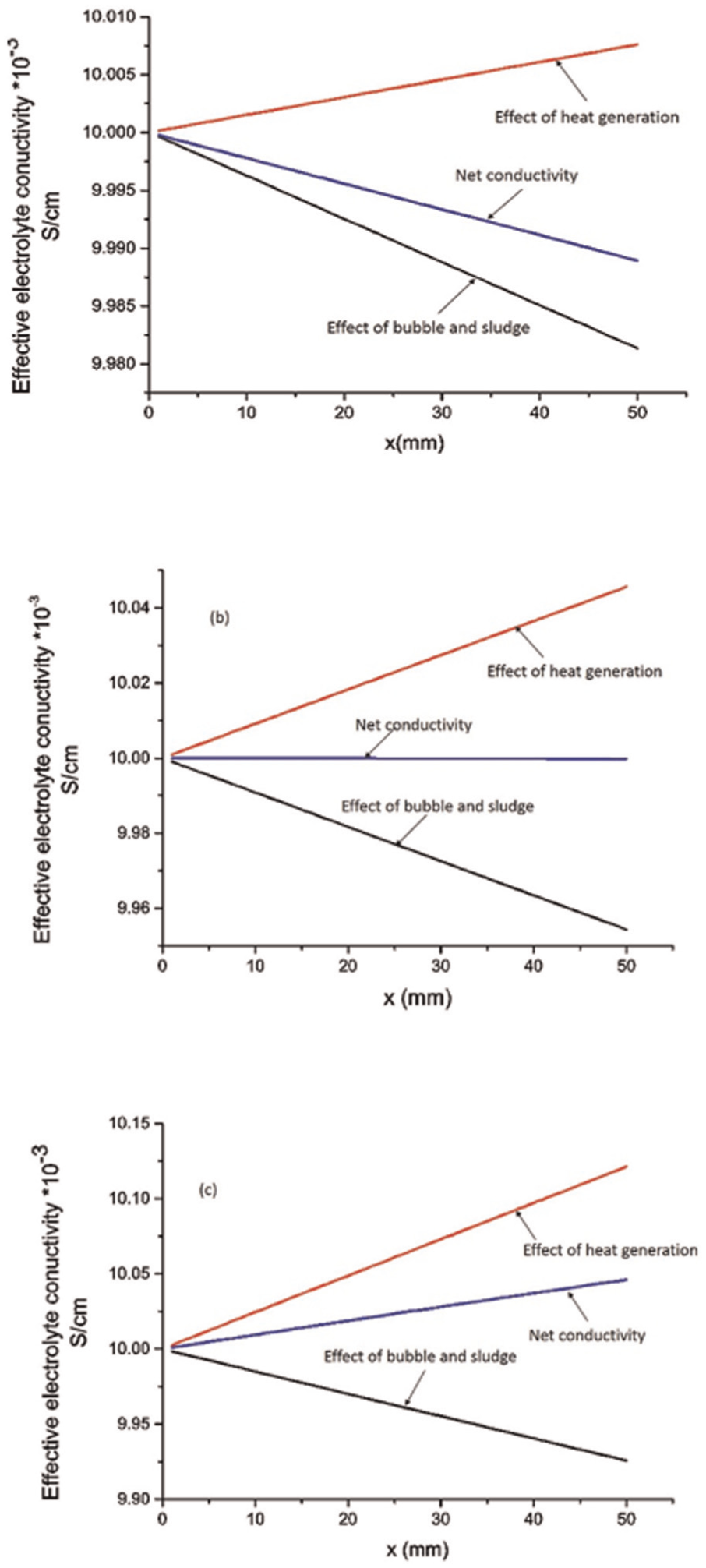
Theoretical relationship for the variation in effective conductivity along the electrolyte flow direction at different input conditions: (a) V = 5 V, IEG = 800 μm, u = 20 m/s; (b) V = 12.25 V, IEG = 800 μm, u = 20 m/s; and (c) V = 20 V, IEG = 800 μm, u = 20 m/s.
Various input parameters of ECM.
In Figure 7(a), the voltage is low, and the effect of sludge and bubbles is dominating the electrolyte conductivity, leading to a net decrease in electrolyte conductivity along the electrolyte flow direction. On increasing the voltage, a point comes when the two opposing effects cancel each other, keeping the electrolyte conductivity value almost constant. In this case, at applied voltage = 12.25 V, the electrolyte conductivity becomes constant along the electrolyte flow direction (Figure 7(b)). However, if the voltage is further increased, the effect of heat generation becomes more dominant than the effect of bubbles and sludge, resulting in overall increase in electrolyte conductivity along the electrolyte flow direction (Figure 7(c)). Here, it is to be noted that the electrolyte conductivity decreases with an increase in sludge volume fraction. However, if the sludge is electrically conductive, the presented results would be quite different.
Conclusion
In this work, the effect of sludge, gas bubbles, and heat on the electrolyte conductivity during ECM has been studied. The conclusions drawn from this work are as follows:
The proposed comprehensive model for the prediction of electrolyte conductivity for the given temperature, volume fraction of bubbles, and volume fraction of sludge are validated and found to agree well with the experimental results.
The reduction in electrolyte conductivity due to the presence of sludge and gas generation can be compensated by the increase in temperature caused due to heat generation during ECM. It is possible to have machining conditions to give almost constant electrolyte conductivity in the machining zone during ECM. This will help in accurate tool design and anode profile prediction for ECM.
During ECM, if the IEG is very small (<200 μm), the electrolyte conductivity reduces by more than 20% at 10 V. Hence, at small IEGs, the effect of bubbles and sludge seems to dominate the effect of heat generation, leading to a net reduction in electrolyte electrical conductivity.
Footnotes
Appendix 1
Acknowledgements
Authors sincerely acknowledge and thank for the help of Mr Divyansh Patel and Mr Leeladhar Nagdev, PhD scholars in Mechanical Engineering Department at IIT Kanpur, during different phases of this work and in the preparation of this manuscript.
Declaration of conflicting interests
The author(s) declared no potential conflicts of interest with respect to the research, authorship, and/or publication of this article.
Funding
The author(s) received no financial support for the research, authorship, and/or publication of this article.