Tool strain–based wear estimation in micro turning using Bayesian networks

Abstract

Estimation of tool wear in micro turning is important as it enhances the process fidelity and the surface quality of the job. In this work, a simple process is demonstrated that estimates the tool wear from strain data near the cutting edge of the tool tip for micro turning operations. The tool strain for tool with six different wear lengths, collected using fiber Bragg grating sensor, was preprocessed to generate a probability distribution. The strain and tool wear data were used as the training dataset. This training dataset was subjected to maximum likelihood estimation algorithm to obtain the conditional probability distribution table required for the functioning of a suitable Bayesian network. The Bayesian network was tested for estimation of tool wear using strain data as priors for three different experiments. The maximum error in tool wear estimation using this procedure was ∼6 µm.

Introduction

Estimation of tool wear in micro machining operations, as compared to conventional scale machining, proves to be a daunting task due to varying process physics, cutting mechanism and miniature sizes of tools.^1,2 In contact-based micro machining processes such as micro turning, micro milling and micro drilling, tool wear is influenced by a number of factors such as type of tool, tool morphology, tool strain, machining conditions and work materials. ³ Unlike conventional scale processes where machining primarily occurs by cutting at the tool edge, micro-scale material removal processes involve three different mechanisms, namely, cutting, slipping and plowing that makes the tool–work interaction complex and therefore drawing proper inference regarding tool wear using machine parameters becomes a difficult task. ⁴

Among all the contact-based micro material removal processes, micro turning has gained significant popularity and utility due to its capability of generating ultra smooth surfaces which finds wide application in fabrication of optical components, aerospace industries and biomedical implants. Tool wear in micro turning reduces the surface integrity of the finished products and leads to higher machining stress which causes inaccurate machining due to tool holder deflection that proves harmful for the machine.^5,6 Furthermore, unexpected tool wear requires frequent alteration of the tool which demands untimely machine shutdown, thereby affecting the supply chain for the finished product. Therefore, a process that estimates tool wear dynamically using micro turning is of utter necessity, such that the aforesaid problems are alleviated and proper efficiency of the micro turning operation is achieved.

Several reports for tool wear estimation in micro cutting operations^7,8 can be found in the literature, and correlation between tool wear and cutting force in diamond turning is very recently reported. ⁹ However, the process for estimation of tool wear specifically for micro tuning operations is not yet available. The surface finish of the product in micro turning is of more importance than the other micro material removal procedures which are generally affected by tool strain caused by cutting edge de-shaping as a result of tool wear. Keeping the above in mind, in this work an approach for wear estimation in micro turning is demonstrated. In the existing literature, different sensors combined with signal processing algorithms are used for measurement of physical parameters for tool wear estimation. Malekian et al. ¹⁰ proposed the use of accelerometers, force and acoustic emission sensors on various locations of the machine along with a neuro-fuzzy approach to determine the state of the tool. The proposed method efficiently estimates the tool wear; however, it needs a long training time for the neuro-fuzzy engine to work accurately. Neural network–based estimation method for tool wear from cutting force signals procured using dynamometer was proposed by Tansel et al. ¹¹ In this method, the training was computationally intensive and it took 151 s to train the neural network as claimed in the reference paper. Very recently, a self-organizing map (SOM)-based algorithm was used on acoustic signals for tool wear monitoring in micro cutting operations. ¹² In this work, class mean scatter criteria were used to combat the system variations and the SOM was used to eliminate the effects of noise. Thus, in this work, two different algorithms were fused to classify the tool wear accurately.

In all of the above approaches, the sensors were placed away from the cutting zone which needs some signal preprocessing for noise removal, thereby making the systems computationally expensive. Various tool wear estimation techniques using theoretical analysis and numerical simulation technologies are depicted in Yen et al. ¹³ However, mere simulations cannot ensure the accuracy of estimated tool wear especially when the tool nose radius is in micron scale because of different process physics in micro cutting. A strategy to estimate tool wear in conventional diamond face-turning was attempted in Scheffer and Heyns, ¹⁴ where an accelerometer and a piezoelectric strain sensor placed close to the cutting tool was used to measure vibration and tool strain, respectively. Although the tool strain was the only relevant tool wear indicator that could be measured closest to the cutting zone for conventional turning as mentioned in the reference paper, use of piezoelectric strain sensor in micro turning is difficult owing to limited footprint of tool near the cutting edge. Strain measurement in micro turning near to the cutting edge demands sensor with footprint in the range of few hundred microns. Fiber Bragg grating (FBG) sensor bears a very limited footprint (typically in few hundred microns). Use of FBG sensors for measurement of temperature, strain, acceleration and so on is well established.^15,16 These facts have inspired us to use FBG sensor for measurement of tool strain in micro turning in our experiments.

Signal processing approaches for estimation of tool wear from the measured data have been attempted using neural networks, ¹⁷ SOMs, ¹⁸ adaptive resonance theory (ART) ¹⁹ and Bayesian networks. ²⁰ A neural network lack semantic interpretability and let the user to consider the system as a black box which renders the signal processing to be complex. SOMs require necessary and sufficient data in order to develop meaningful clusters which may not be universally possible in tool wear estimation. Few of the ART models have drawbacks which involve outputs influenced by the order of training dataset. A Bayesian network, on the other hand, proves to be highly advantageous for estimation of tool wear and may therefore be considered superior to other known methods. Some of its advantages include optimal decision making capability, robustness to parameter changes, semantic interpretability, flexible applicability and ability to interpret parameters from missing data. ²¹ Therefore, we chose Bayesian network for this work.

In this work, the tool strain data measured using FBG sensor and the wear measured from microscope images of the tool for the particular set of experiments were normalized to generate a training dataset. The training dataset was used to obtain the conditional probability distribution table (CPT) for a Bayesian network using maximum likelihood estimation (MLE) algorithm. The trained Bayesian network was supplied with tool strain data for experiments with different tool wear to estimate the tool wear values.

This article is divided into five sections. The “Methodology” section explains the detailed method of tool wear estimation. The “Results” section demonstrates the output of the Bayesian network in tool wear estimation. The inferences collected from the experiments and their significance are stated in the “Discussion” section. This article is finally concluded in the “Conclusion” section.

Methodology

In our work, variation in strain measured near to the cutting edge of the tool tip (ε) using FBG sensor was used for estimation of tool wear. Six tools with different wear lengths were used for micro turning of a mild steel rod (standard: IS 2062, grade: Fe 410WB) with fixed machining parameters. Experiments were conducted eight times for each tool with same machining parameters, rendering us with 48 strain datasets. The difference in strain value between the consecutive samples (Δε) for each dataset was computed. These strain difference datasets (Δε) serve as training set for the Bayesian network. Four bin normalized histograms with equal bin size were generated for each of these strain difference datasets. Each bin denotes the number of normalized strain difference data lying in the range of the bin limits (0–0.25, 0.25–0.5, 0.5–0.75 and 0.75–1). The variance of data for each bin was computed for 48 datasets. Two bins with highest variance were considered for further data processing. The tool wear was measured from microscope images for each of the six tools. The strain difference data along with the tool wear were considered features for further training and signal processing. A learning matrix was generated which contained the magnitude of two bins with highest variances and the tool wear length. The training dataset was subjected to MLE algorithm to generate a CPT (conditional probability table) for the Bayesian networks. This completes the learning paradigm of the proposed Bayesian network. The Bayesian network was fed with strain difference data for three other tools (test tools) with different tool wear as priors to estimate the wear length. The estimated wear length was then compared with the measured wear length to find the possible errors in estimation. The methodology is depicted in Figure 1.

Figure 1.

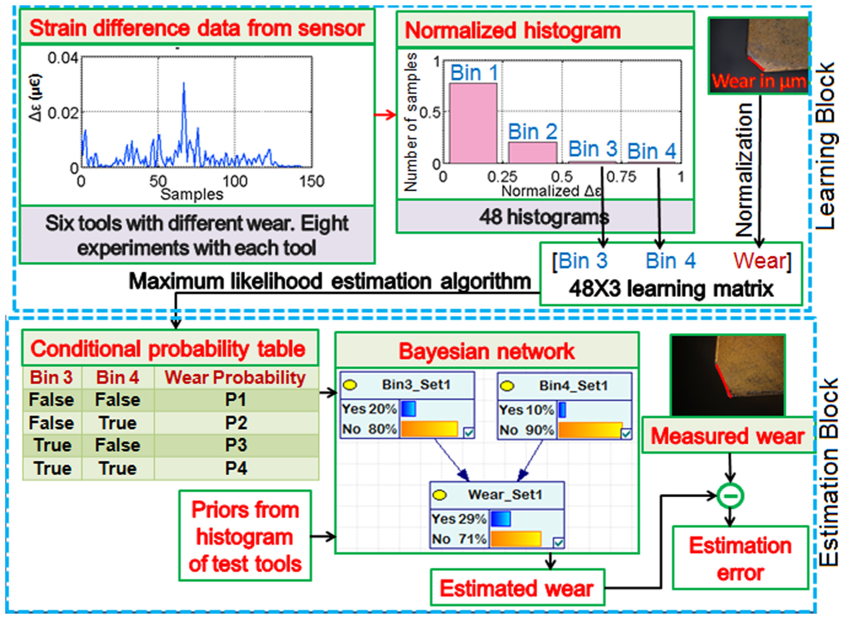
Methodology for tool wear estimation used in this work.

Before proceeding further, each of the blocks for strain data collection and estimation algorithms are explained in detail in the subsequent subsections.

Strain measurement using FBG sensor

In this work, the strain near to the cutting edge of the tool tip was measured using a FBG sensor. A FBG sensor works on the principle of Fresnel’s diffraction. It consists of an optical fiber with spatial modulation of refractive index. ²² This modulation causes a specific wavelength of broadband light incident on the gratings to get reflected back. Variations in temperature or strain result in the shift in wavelength of reflected light. The wavelength shift is measured using an interrogation circuitry to get the values of strain and temperature. FBG sensors possess cross sensitivity to strain and temperature. Elimination of cross sensitivity can be conducted by various methods, the use of two FBGs of different strain and temperature sensitivities being the simplest. This paradigm was used to measure strain and temperature in this research.

The elimination of cross sensitivity effect for temperature near to the cutting edge of the tool tip was conducted using a standard FBG-based temperature probe (Micron optics OS4210). Unlike miniature-sized temperature probes, FBG-based standard strain sensors are larger and difficult to be accommodated near the tool tip. The problem was alleviated using a Germanium-doped bare FBG sensor fabricated in-house pre-calibrated using a standard FBG strain sensor (OS3110) and temperature sensor (OS4210). The strain sensitivity of OS3100 and the temperature sensitivity of OS4210 are 1.4 pm/µε and 10 pm/°C, respectively. The fabricated FBG operates at 1517 nm nominal wavelength. The strain and temperature sensitivities for the fabricated FBG were found to be 1.137 pm/µε and 11.347 pm/°C, respectively. The sensors were attached rigidly in the tool notch using Araldite adhesive. NI-based FBG interrogator (PXIe 4844) was used for National Instruments sensor interrogation. The interrogator measures the shift in nominal wavelength for the FBG sensors. Strain values were obtained from the wavelength shifts of the FBG sensors using equations (1) and (2). ²³ The strain value obtained in a sample was subtracted from the next sample to get Δε (difference in strain between the samples) values as in equation (3)

$$\frac{\Delta {\lambda }_{B1}}{{\lambda }_{B1}}=C_{T1}\Delta T$$

(1)

$$\frac{\Delta {\lambda }_{B2}}{{\lambda }_{B2}}=C_{s2}\epsilon +C_{T2}\Delta T$$

(2)

$$\Delta \epsilon ={\epsilon }_{i+1}-{\epsilon }_i$$

(3)

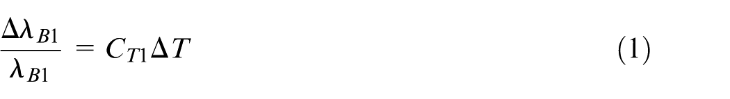
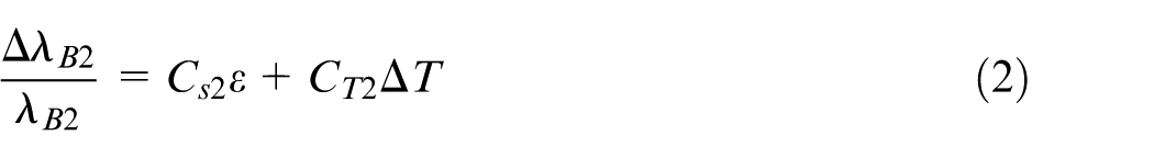
The subscript 1 represents the FBG temperature sensor (OS4210) and the subscript 2 represents the bare FBG sensor which has both strain and temperature sensitivities. λ_B is the nominal wavelength, Δλ_B is the shift in nominal wavelength, C_T and C_s are temperature and strain sensitivities, ε and ΔT are the strain and temperature, respectively. The subscript i denotes the ith sample.

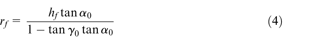
The experimental setup consists of a three-axis system for micro turning operations. Three-axis linear translation stages supplied by Holmarc company (Model number MTS90115-2) driven by stepper motors was used in this work. A homemade driver-controller system was designed for driving the setup. The spindle used in the system was able to rotate at a maximum speed of 7000 r/min. The tool used for machining was a cemented carbide turning insert procured from Sandvik Coromant (Part No. MAFL3010 1025). The tool has a notch near the cutting edge where the FBG sensors were rigidly attached. Micro turning operations were conducted for mild steel rod (standard: IS 2062, grade: Fe 410WB) with 50 mm/min feed rate, 100 µm depth of cut and 2000 r/min as spindle speed. Experiments were conducted for tools with six different wear lengths, the wear lengths being artificially generated by grinding the cutting edge of the tool tip. Artificial tool wear generation for wear study is well established as it saves experimentation time and is claimed to be an accurate and effective method in earlier research. ²⁴ To obtain natural wear pattern on the cutting edge of the tool, grinding was carefully conducted so as to satisfy the primary relation between rake angle (γ₀), clearance angle (α₀), length of flank wear (h_f) and radial wear length (r_f) as in equation (4) and Figure 2

$$r_f=\frac{h_f\tan {\alpha }_0}{1-\tan {\gamma }_0\tan {\alpha }_0}$$

(4)

Figure 2.

Conventions for determination of wear length.

In our experiments, the rake angle of the tool was 0° and the clearance angle was 9°. So, equation (4) can be rewritten as equation (5)

$$h_f=6.31r_f$$

(5)

For each tool, the experiments were conducted eight times, thus rendering 48 datasets in total. The experimental setup is shown in Figure 3.

Figure 3.

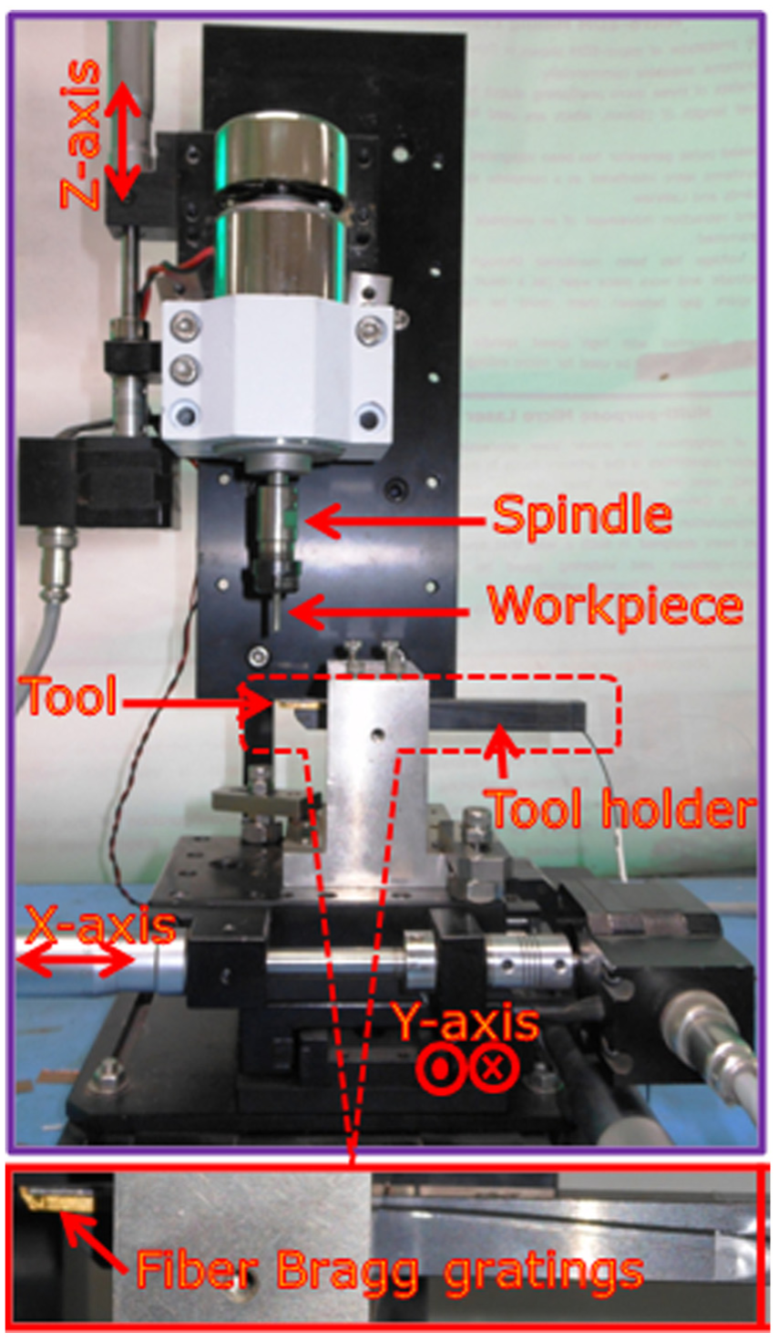
Experimental setup for measurement of strain using FBG sensors in micro turning.

Feature extraction and signal processing

The difference in strain signals versus number of samples (Δε) for 48 sets was subjected to feature extraction. Each of the signals was normalized to their maximum values and a normalized histogram with four bins (distribution range) was constructed in MATLAB. The X-axis of the histogram shows the magnitude of Δε normalized to the maximum strain value of each set, whereas the Y-axis shows the normalized number of samples lying in the particular bin. A total of 48 histograms each with four bins were thus generated. The variance of each bin for 48 sets was calculated. The two bins with highest variances were taken as strain feature. The wear lengths of six tools used in our experiments were measured from tool tip images captured under Olympus BX 51M microscope and its allied software. To keep the measurements consistent every time, a tool holder was developed for placement of tool at the same location under the microscope. The setup for tool wear measurement is shown in Figure 4. The wear length served as a feature for training dataset. A 48 × 3 matrix was thus generated as training dataset (T) as in equation (6)

$$T=\left[\begin{array}{ccc}\hfill \mathrm{Bin}3\hfill & \hfill \mathrm{Bin}4\hfill & \hfill \mathrm{Wear}\hfill \end{array}\right]$$

(6)

Figure 4.

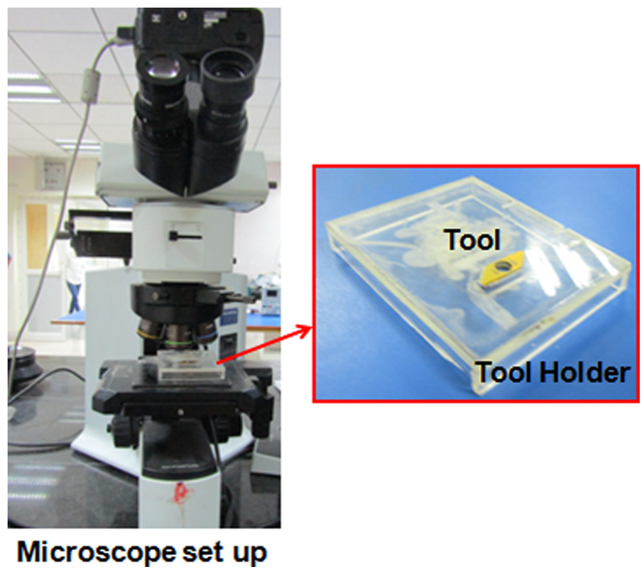
Setup for tool wear measurement.

Bayesian network training and development

A Bayesian network is a probabilistic model that represents a number of random variables and their conditional dependencies using a directed acyclic graph (DAG). The network finds the posterior probability distribution from prior probability distribution and likelihood. ²⁵ The likelihood is a set of conditional probability distributions that defines the dependency between the priors and posteriors and is represented in form of a conditional probability distribution table (CPT). In our experiments, the classified signals (magnitude of two selected bins of the histogram) and the tool wear were considered as the priors and posteriors, respectively. The relationship between them was governed by a CPT. In general, the CPT is generated through appropriate guidance from a well-versed expert in the respective domain of interest. However, in micro turning, no expert can define the relationship between strain variables and the tool wear due to huge uncertainties in nature of strain data and miniature size of tool that are difficult to be visualized. This demands an automated system for generation of CPT from the training dataset depicted in the previous subsection.

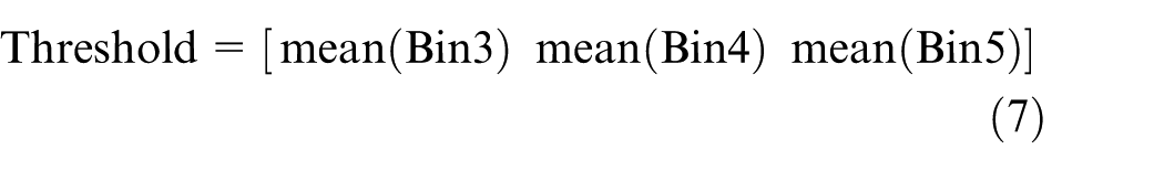
Generation of CPT from training dataset was conducted using MLE algorithm employing Bayesian network toolbox in MATLAB. MLE paradigm was preferred over other methods for CPT generation as the approach is simple, unbiased and the paradigm achieves smallest possible variance among any unbiased estimator. ²⁶ The training dataset was discretized by setting mean of the training dataset as a threshold as in equation (7)

$$\mathrm{Threshold}=[\mathrm{mean}(\mathrm{Bin}3)\mathrm{mean}(\mathrm{Bin}4)\mathrm{mean}(\mathrm{Bin}5)]$$

(7)

After thresholding of the discrete training dataset, it consisted of arrays of “0” and “1.” The maximum likelihood for a discrete dataset was calculated using equation (8) ²⁷

$$\Theta =\frac{P_1}{P_1+P_0}$$

(8)

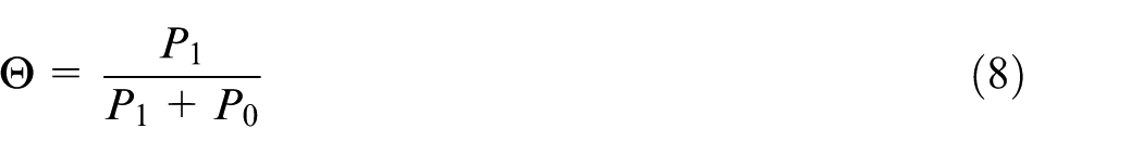
where P₁ denotes the number of data for which the posterior is true given its priors, P₀ denotes the number of data for which posterior is false for given set of priors and Θ is the maximum likelihood. A CPT is obtained in this process.

Tool wear estimation

The Bayesian network fused with calculated CPT was used to estimate the tool wear for experiments with tool of three different wear lengths. The strain near to the cutting edge of tool tip was measured for the test tools for same machining parameters as during training and similar histograms were generated for test strain data. The data value of “Bin 3” and “Bin 4” were priors for the Bayesian network. The Bayesian network estimated the posteriors (tool wear) using the Bayes theorem given in equation (9) ²⁸

$$\begin{array}{c}\multicolumn{1}{c}{P[\mathrm{Wear}=\mathrm{yes}]=\sum _{\mathrm{Bin}3,\mathrm{Bin}4}P[\mathrm{Wear}=\mathrm{yes},\mathrm{Bin}3,\mathrm{Bin}4]}\\ \multicolumn{1}{c}{=P(\mathrm{Wear}|\mathrm{Bin}3,\mathrm{Bin}4)\times P(\mathrm{Bin}3,\mathrm{Bin}4)}\\ \multicolumn{1}{c}{+P(\mathrm{Wear}|\mathrm{Bin}3,\overline{\mathrm{Bin}4})\times P(\mathrm{Bin}3,\overline{\mathrm{Bin}4})}\\ \multicolumn{1}{c}{+P(\mathrm{Wear}|\overline{\mathrm{Bin}3},\mathrm{Bin}4)\times P(\overline{\mathrm{Bin}3},\mathrm{Bin}4)}\\ \multicolumn{1}{c}{+P(\mathrm{Wear}|\overline{\mathrm{Bin}3},\overline{\mathrm{Bin}4})\times P(\overline{\mathrm{Bin}3},\overline{\mathrm{Bin}4})}\end{array}$$

(9)

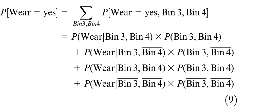
In equation (7), P(Wear| Bin 3, Bin 4) denotes the wear probability subject to Bin 3 and Bin 4 being true and this is obtained from the CPT. The term P(Bin 3, Bin 4) denotes the priors. All other terms carries the similar meaning. P [Wear = yes] denotes the estimated probability of tool wear. The estimated tool wear was compared with measured tool wear for the tools using microscope images and software as followed in previous sections.

Results

The six different tool wear lengths obtained from tool images using microscope for Bayesian network training are shown in Figure 5.

Figure 5.

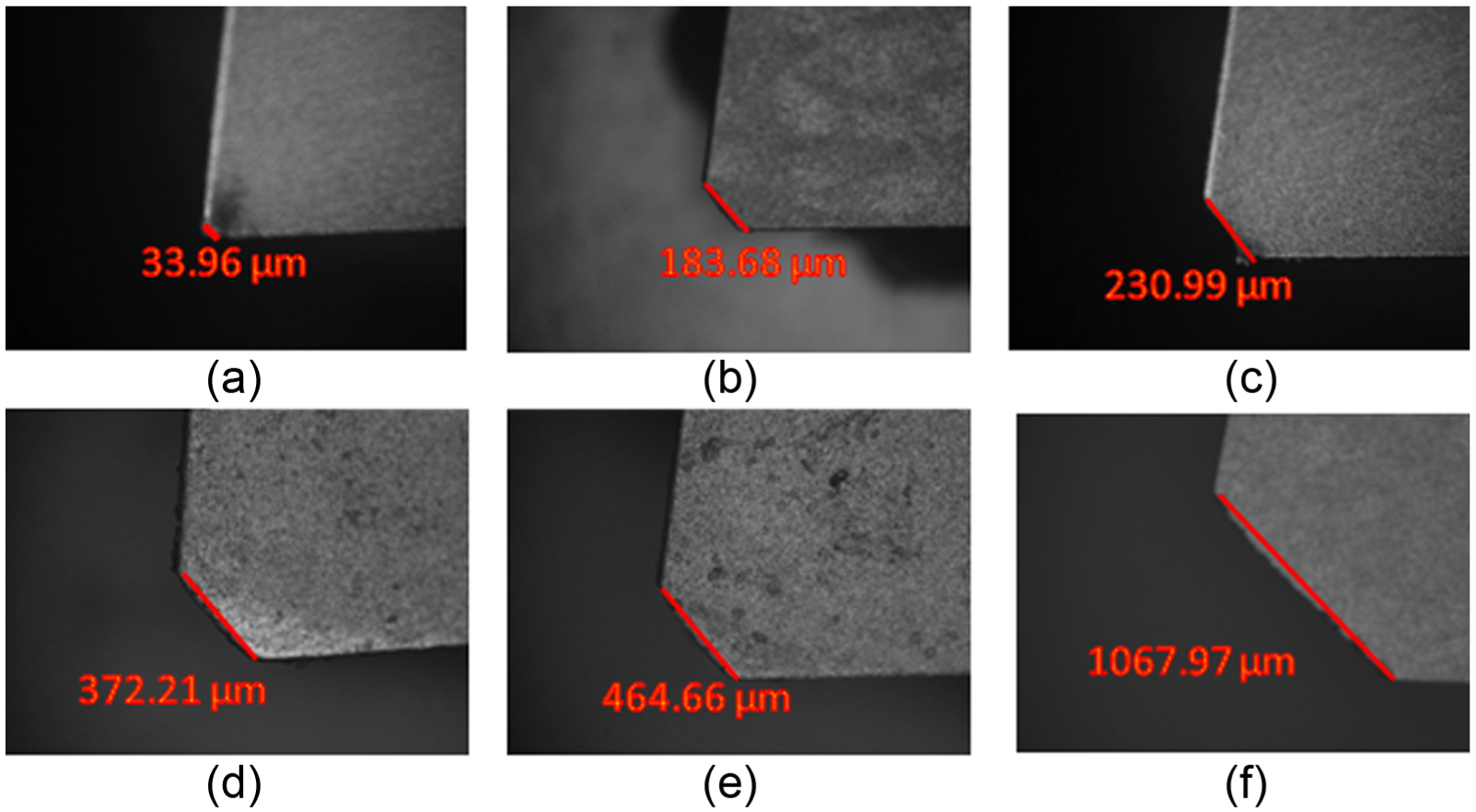
Tool wear length using microscope image for six different wear lengths used in Bayesian network training. Wear lengths are found as (a) 33.96 μm, (b) 183.68 μm, (c) 230.99 μm, (d) 372.21 μm, (e) 464.66 μm, (f) 1067.97 μm.

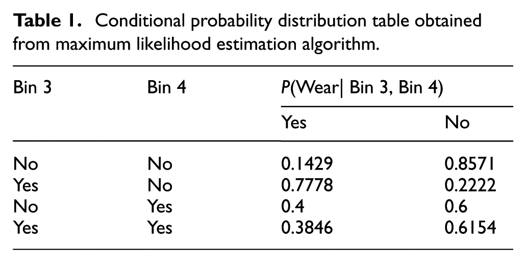
The generated Bayesian network involving priors as test data and the CPT is shown in Figure 6. The Bayesian network estimated the wear as a percentage of maximum wear length. The maximum wear was obtained as 1067.97 µm as in Figure 5. The estimated wear is shown in Figure 7. The generated CPT is shown in Table 1.

Figure 6.

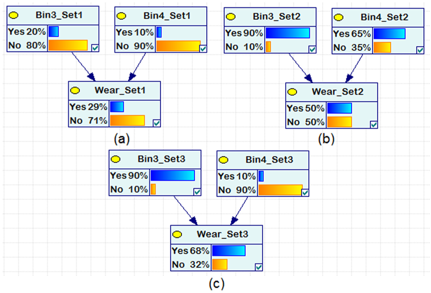
Bayesian network for three different experimental tests of tool wear using (a) Test tool 1, (b) Test tool 2, and (c) Test tool 3.

Figure 7.

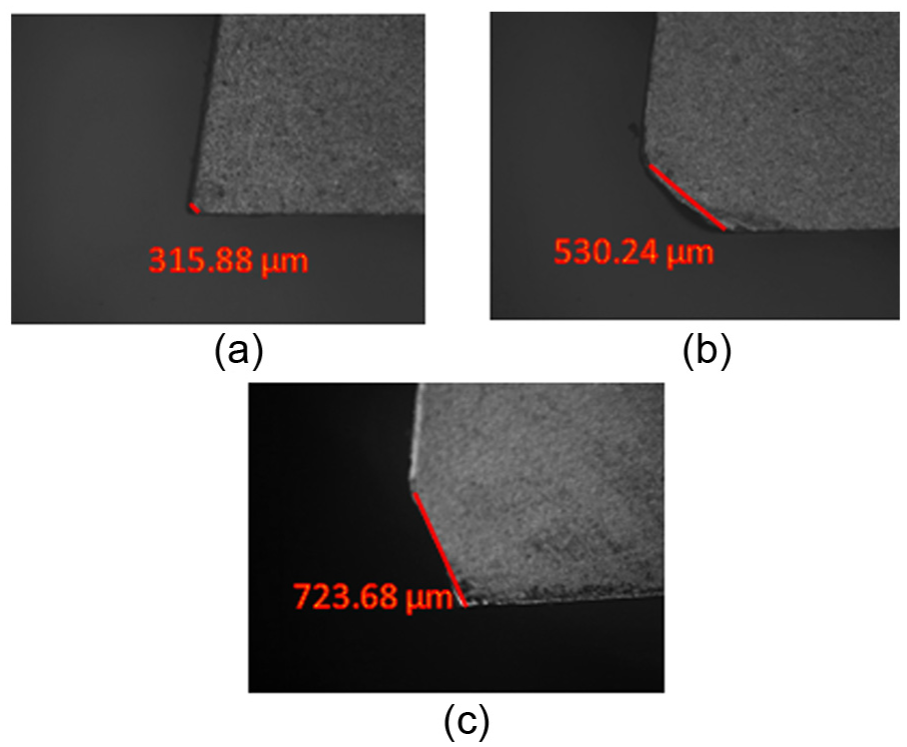
Tool wear images observed under microscope for (a) test tool 1, (b) test tool 2, and (c) test tool 3.

Table 1.

Conditional probability distribution table obtained from maximum likelihood estimation algorithm.

Bin 3	Bin 4	P(Wear| Bin 3, Bin 4)
		Yes	No
No	No	0.1429	0.8571
Yes	No	0.7778	0.2222
No	Yes	0.4	0.6
Yes	Yes	0.3846	0.6154

The measured tool wear for the three tools for which the estimation was conducted is shown in Figure 7.

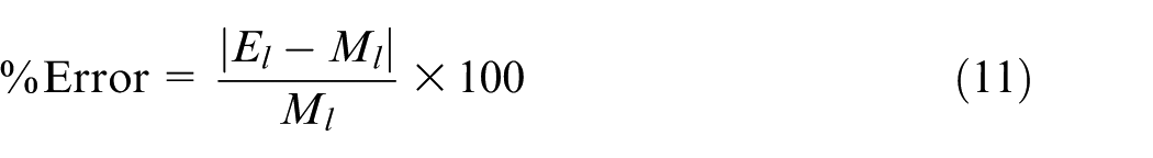
The estimation error in tool wear for the test tools is presented in Figure 8. The estimation error was calculated from estimated wear length (E_l) and measured wear length (M_l) using equations (10) and (11)

$$\mathrm{Error}=|E_l-M_l|$$

(10)

$$\%\mathrm{Error}=\frac{|E_l-M_l|}{M_l}\times 100$$

(11)

Figure 8.

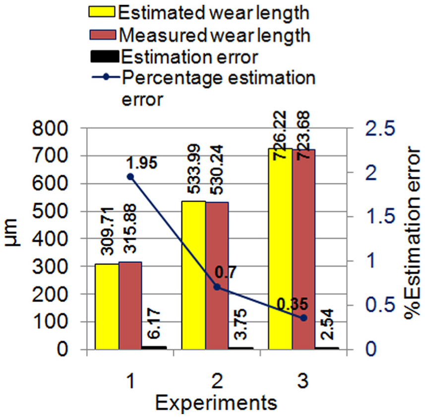
Estimation errors in tool wear for the test tools.

Discussion

The following facts could be inferred from the experiments and the results:

1. Due to factors like miniature footprint, zero interference from other signals and high sensitivity of FBG sensor, it is suitable for strain measurement near to the cutting edge of the tool tip during micro machining operations. The strain measurements were almost free from noise signals due to nearness of the sensor to the cutting zone which would not be the case if other sensors with larger footprint were used. This was the primary reason that the Bayesian network–based proposed method for wear estimation did not require any specific noise filtering paradigms which are commonly used in other wear estimation methods, thereby decreasing the computational load in the estimation job.

2. The number of strain difference signals in Bin 3 and Bin 4 was prominent indicator of tool wear in the conducted experiments. In Figure 6(a), the signal probabilities in Bin 3 and Bin 4 were 20% and 10%, respectively, whereas in Figure 6(b), the probabilities were 90% and 65%, respectively. The estimated wear increased from 29% to 50% due to this difference. On the other hand, in Figure 6(b), the signal probabilities in Bin 3 and Bin 4 were 90% and 65%, respectively, whereas in Figure 6(c), the probabilities were 90% and 10%, respectively. The estimated wear increased from 50% to 68% due to this variation. Thus, increase in probability of Bin 3 and decrease in probability of Bin 4 increases the estimated wear probability.

3. The MLE algorithm was efficient in training the Bayesian network used in our experiments. The generated CPT (Table 1) along with the priors fed to the Bayesian network was capable of detecting the tool wear from strain data with high accuracy. This was due to the robustness of MLE algorithm to small strain signal variations which occurs in experimental process.

4. The maximum estimation error was ∼6 µm which is much lesser than 75 µm reported in reference paper. ²⁹ The percentage error is less than 2% (Figure 8) which shows that the approach is accurate for tool wear estimation in micro turning.

5. The estimation error reduces with the increase in tool wear length to be estimated (Figure 8). For the tool with estimated wear length of 309.71 µm, the estimation error was 1.95%, whereas for the tool with estimated wear length of 726.22 µm, the estimation error was 0.35%. This might be due to higher measurement errors which creep into measurements when the tool wear length is small.

Conclusion

Estimation of tool wear in micro machining operations is a prime requirement in industrial machining centers especially those involved in batch production of various micro parts. In this work, a simple, robust and computationally inexpensive estimation system is proposed for micro turning which uses the strain data procured near to the cutting edge of tool tip measured using FBG sensor to estimate tool wear.

Unlike other delicate and sophisticated sensors, FBG sensors have miniature footprint, are able to operate in adverse conditions and are immune to noise. Hence, such sensors are apt for shop floor applications. The Bayesian network–based estimation system is accurate and requires simple learning strategy for its operation. The MLE algorithm is efficient in CPT calculation. Unlike other applications of Bayesian networks where expert advice is essential for generation of conditional probability distribution, the paradigm suggested in this work is self-sufficient in generation of neighborhood from pre-recorded data.

The suggested paradigm does not require data filtering steps as the strain is captured very near to the cutting edge due to the use of FBG sensor and hence the data are free from unnecessary perturbation and noise. This makes the paradigm computationally inexpensive. The maximum inaccuracy in estimation of tool wear from the strain data was limited to 2% which ensured the applicability of the process in wear estimation.