Sage Journals: Discover world-class research

Abstract

In order to increase the machining accuracy of slow tool servo turning of complex optical surface, the optimal design for tool path was studied. A comprehensive tool path generation strategy was proposed to optimize the tool path for machining complex surfaces. A new algorithm was designed for tool nose radius compensation which had less calculation error. Hermite segment interpolation was analyzed based on integrated multi-axes controller, and a new interpolation method referred to as triangle rotary method was put forward and was compared with the area method and three-point method. The machining simulation indicated that the triangle rotary method was significant in error reduction. The interpolation error of toric surface was reduced to 0.0015 µm from 0.06 µm and sinusoidal array surface’s interpolation error decreases to 0.37 µm from 1.5 µm. Finally, a toric surface was machined using optimum tool path generation method to evaluate the proposed tool path generation method.

Keywords

Complex optical surfaces slow tool servo tool path generation Hermite segment interpolation tool compensation

Introduction

Complex optical surfaces can be used in optical systems to acquire high-quality image, improve the performances, decrease the expense and reduce the size of the system. Ultra-precision machining of the complex optical surfaces has become very important in recent years because of the increased use of complex optical surfaces in many fields such as optics, medicine, and fiber telecommunication and life science.¹

At present, the machining methods for complex surfaces have been developed greatly in industrial and academic fields such as micro-milling, fly-cutting, fast tool servo (FTS) and slow tool servo (STS). Among these technologies, STS is widely utilized for machining many different types of freeform surfaces due to its advantages of high surface accuracy and high machining efficiency. A lot of research was carried out such as the machining experiments of new or complex surface, new lath structure and new application areas. Besides, machining parameters, control system algorithm and tool–workpiece vibration have significant effects on the tool wear and machining accuracy, so relevant research for STS/FTS was also studied.^2
–4

Tool path generation (TPG) method has a direct impact on the surface accuracy for STS/FTS, so relative researches were carried out in recent years. Neo et al.⁵ proposed an attractive solution with an integration of Visual Basic for Application programming interface into SolidWorks to generate spiral tool trajectory for STS/FTS turning of freeform surfaces. According to the surface scallop height, Liu et al.⁶ described a changing feed-rate tool path for FTS, which is a creative idea for TPG for STS/FTS. Zhang et al.⁷ used coordinate transformation to produce the tool path of off-axis aspheric mirrors and reduced the ratio of sag height to diameter. Keong et al.⁸ described a novel FTS diamond turning method with layered tool trajectories to extend the limited stroke length without modifying an existing FTS system. Although there are many different types of TPG methods, the main route of the TPG can be summarized as the following three steps: cutting contact points (CCPs) discretization, tool geometry compensation and the interpolation among discrete cutting location points (CLPs).

Reasonable CCP discretization method is the basis of TPG. For three-axes turning freeform surfaces, spiral tool path is the most typical method.⁹ Both equal angle discretization method and equal arc length discretization method can be used to create discrete rotation points during TPG for STS turning.^10

–13 But the papers did not systematically studied the weakness of the two discretization methods and proposed the solution method. For tool geometry compensation, Fang et al.¹⁴ used the vector mathematics method to compensate tool geometry, including the tool radius compensation and rake angle compensation, but the compensation algorithm is relatively complex. Guan¹ provided the X-stable method to compensate tool radius; however, he did not do the experiment to prove it. According to the X-stable method, Wang¹⁵ proposed an algorithm to compensate the tool nose radius. Because the spline interpolation is used, the algorithm has relatively large calculation error. Hu et al.¹⁶ used non-uniform rational B-spline (NURBS) interpolation to improve the surface accuracy of the freeform surface, but did not dealt with the interpolation among discrete CLPs. Zhang et al.¹⁷ evaluated B-spline interpolation method, and B-spline does not pass specified interpolation nodes on the cutting location trajectory, so that the B-spline interpolation leads to relatively larger interpolation error. Guan¹ and Wang et al.¹⁸ proposed Hermite interpolation method, but it cannot ensure the interpolation path two-order continuous.

In this article, the TPG method for STS turning was systematically studied. This method comprises the determination of CCPs, compensation of the tool geometry, analysis of the entrance parameter algorithm of position–velocity–time (PVT) mode, machining simulation study and validation of the actual machine.

STS turning technology

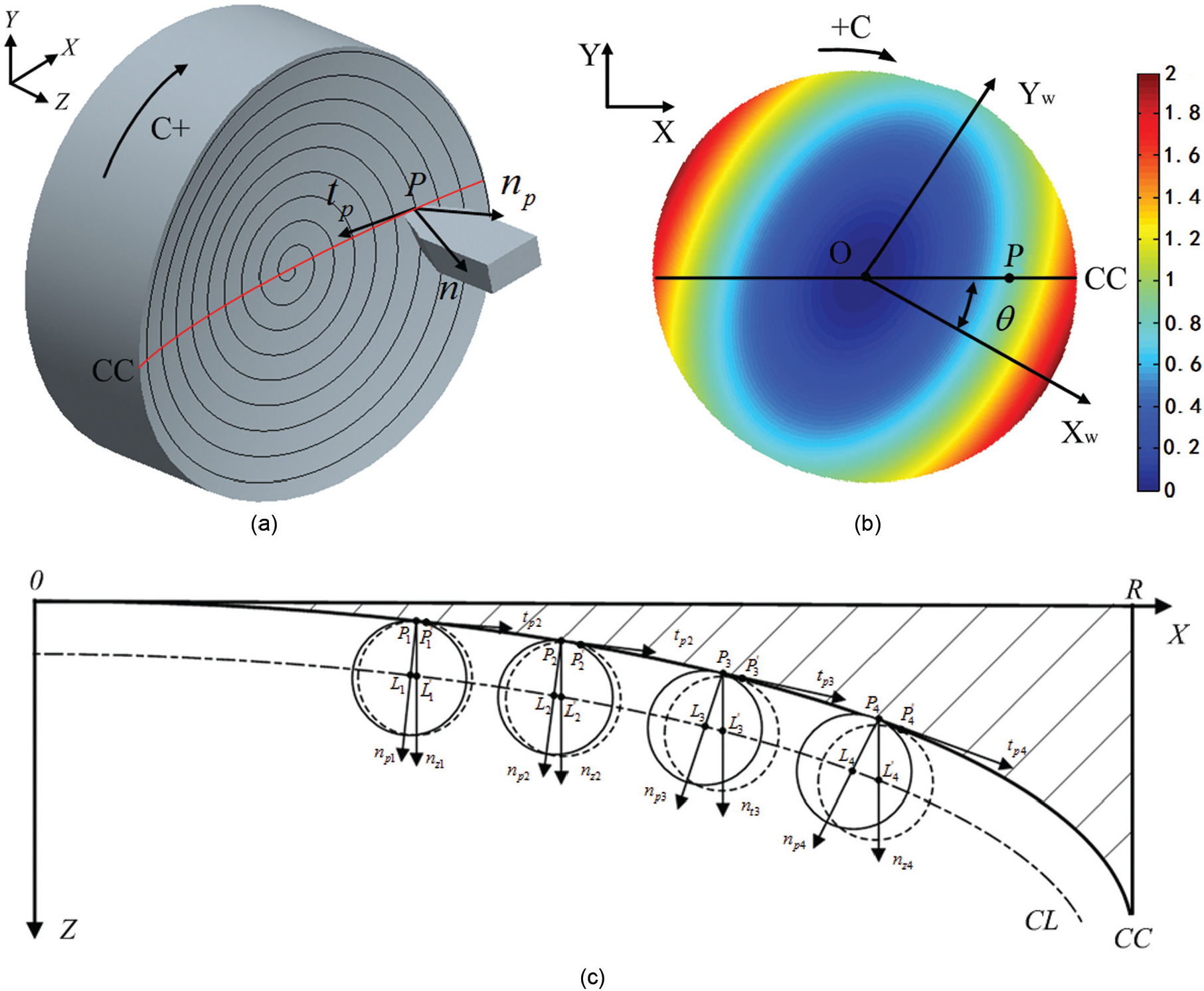
The STS turning technology is a precision turning method with high accuracy and high efficiency. Figure 1(a) shows the schematic diagram of the mechanical system setup of STS turning used in this study, which has a linear X-axis, a linear Z-axis and a rotary C-axis. The complex surface can be machined by controlling the X-axis, the Z-axis and the C-axis simultaneously. The schematic diagram for control system setup of the STS turning is shown in Figure 1(b). Because the motion accuracy of the Z-axis has most important influence on the machining error, Z-axis has both position feedback and speed feedback to ensure its motion accuracy. The numerical control (NC) program includes the information of the CLPs. According to the NC program, the integrated multi-axes controller (IMAC) performs an interpolation computation between two neighboring points and controls the three axes of the setup to generate the complex surfaces.

Figure 1.

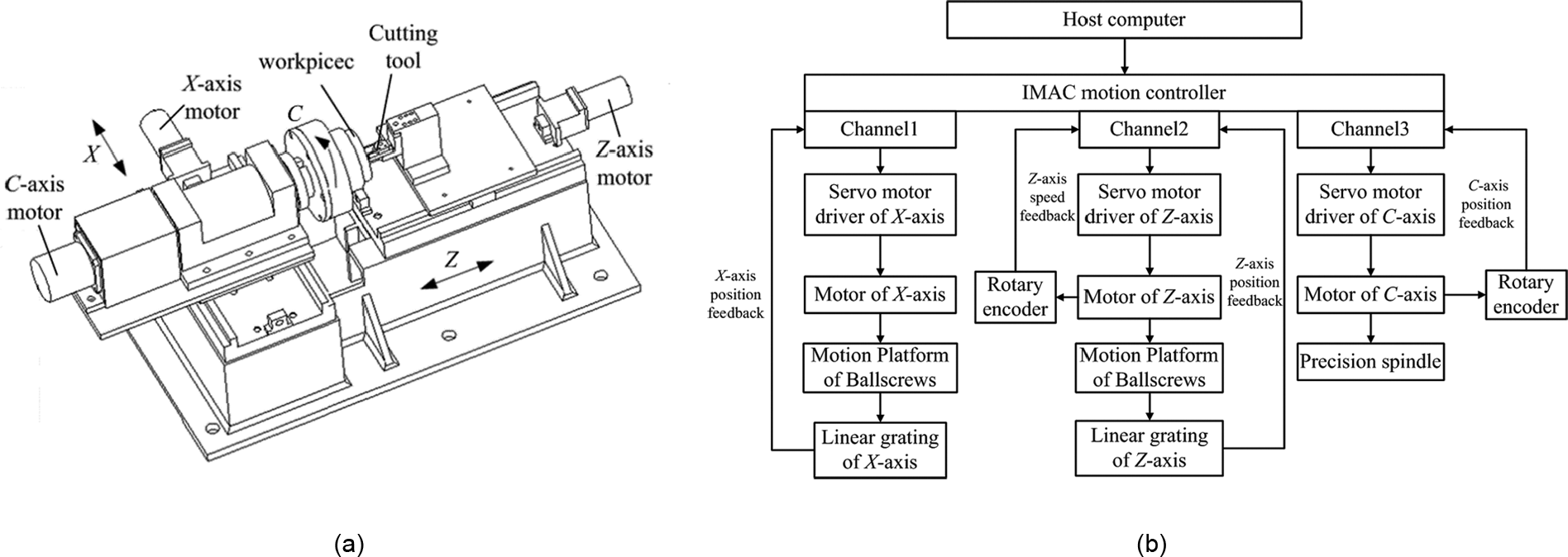
Schematic diagram of STS turning for complex surfaces: (a) mechanical system and (b) control system.

TPG

The TPG for turning complex surfaces mainly consists of mathematical expression of the complex surfaces, CLPs optimization and turning trajectory interpolation. Figure 2 is the schematic diagram of the TPG for turning complex surfaces. First, the complex surfaces should be expressed by scalar equation or parameter vector equation in polar coordinates or Cartesian coordinates. The CLPs optimized planning includes two steps: first, calculating the CCPs on the complex surface and then calculating the CLPs using the tool geometry compensation principles. There are three methods to discrete CCPs and two methods for compensating the tool geometry error. The discretization methods include the equal angle discretization method, the equal arc length discretization method and the integrated discretization method. The tool geometry compensation method includes normal direction compensation and Z-direction compensation. The IMAC can provide SPLINE method and PVT method to interpolate trajectory.¹⁹ The SPLINE interpolation only needs the coordinate value of each axis and time interval between two adjacent CLPs to calculate the coordinate value of interpolation points. The PVT method needs to be provided velocity value of each CLP in addition. In order to acquire accurate cutting trajectory, three entrance parameter algorithms of the PVT method are analyzed: area method, three-point method and triangle rotary method; the triangle rotary method was put forward by the authors, which can create more accurate trajectory than the other methods. The verified NC program was exported finally.

Figure 2.

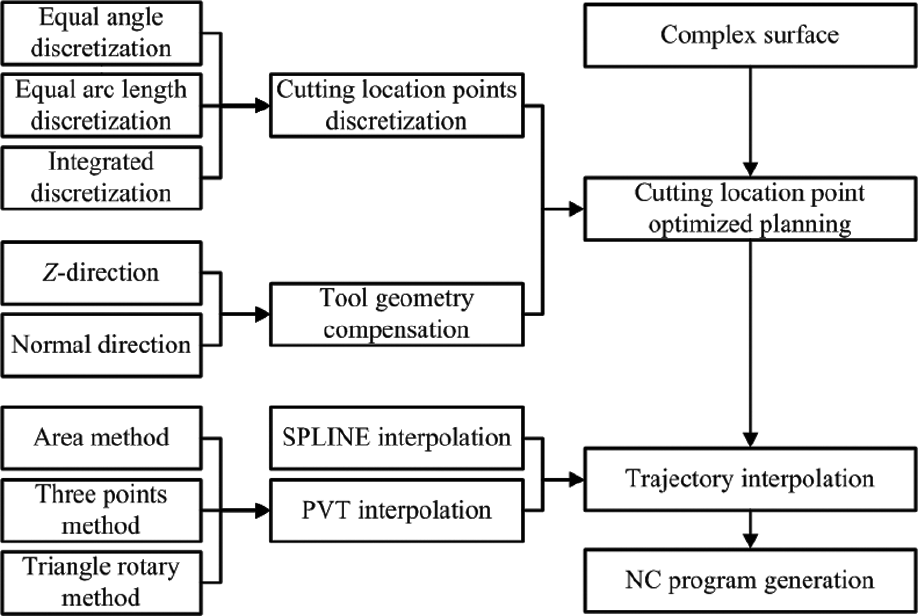
Schematic diagram for STS tool path generation.

CCP generation

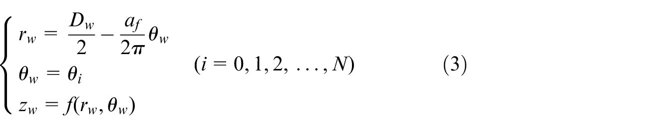
The CCPs are the position point on the workpiece’s surface, which contacts the diamond tool. The tool contact path represents the tangential trajectory between the diamond tool and the machined surface. Nowadays, the cutting tool path planning methods mainly contains equal parametric line method, equal section method, equal spacing method and equal residual height method.¹⁵ The C-axis is the rotating axis, so the equal spacing method is the better option. In this case, the CCPs trajectory is uniformly distributed, which involves less calculation and possesses high machining efficiency. The CCPs trajectory is described in Cartesian coordinates as follows

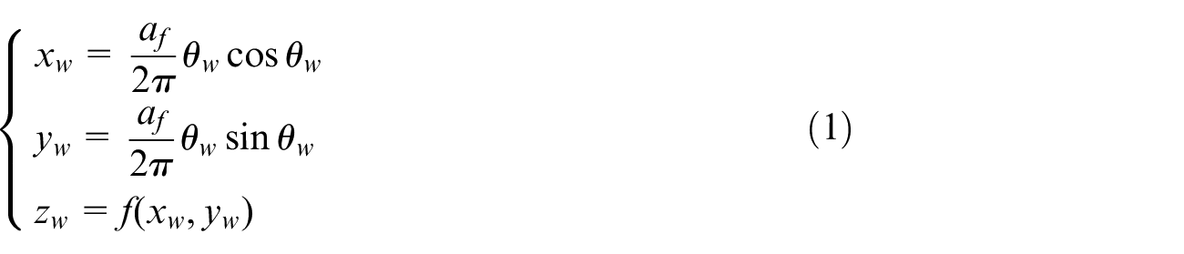
{\begin{matrix} x_{w} = \frac{a_{f}}{2 π} θ_{w} \cos θ_{w} \\ y_{w} = \frac{a_{f}}{2 π} θ_{w} \sin θ_{w} \\ z_{w} = f (x_{w}, y_{w}) \end{matrix}

(1)

where a_f is the feed rate of X-axis, θ_w is the angle between X-axis and the line from the CCPs to the workpiece center and z_w = f (x_w, y_w) is the mathematical description of complex surface.

IMAC NC system can only process the movement between designated points, so the CCPs trajectory must be described. The tool contact path can be discretized by different methods, such as equal angle discretization, equal arc length discretization and integrated discretization.

Equal angle discretization method

As it is shown in Figure 3(a), equal angle discretization method means that the angle Δθ between adjacent CCPs is equal. The CCPs trajectory after equal angle discretization is as follows

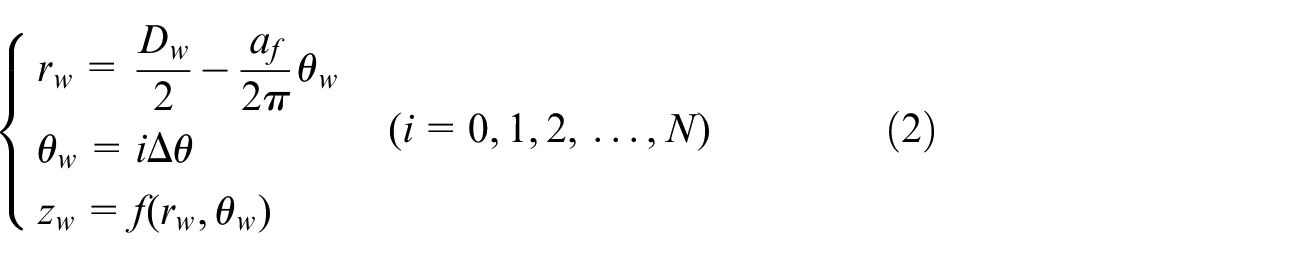
{\begin{matrix} r_{w} = \frac{D_{w}}{2} - \frac{a_{f}}{2 π} θ_{w} \\ θ_{w} = i Δ θ \\ z_{w} = f (r_{w}, θ_{w}) \end{matrix} (i = 0, 1, 2, \dots, N)

(2)

where (r_w, θ_w, z_w) is the three-dimensional (3D) contour coordinate value of complex surface in cylindrical coordinate system, D_w is the diameter of workpiece, z_w = f(r_w, θ_w) is the cylindrical coordinate function of complex surface, r_w is the distance between CCP and center of workpiece, θ_w is the angle which start counting from the “cut in point,” and Δθ is the increase in angle between adjacent points.

Figure 3.

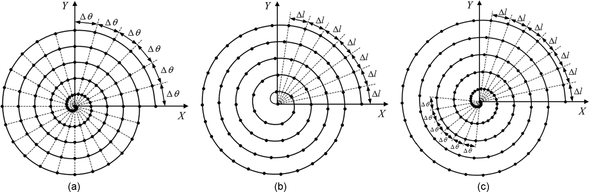
Schematic diagram of different discretization method: (a) equal angle discretization method, (b) equal arc length discretization method and (c) integrated discretization method.

The advantages of the equal angle discretization are the simple calculation and easy to evaluate. But the trajectory points close to the central region are too dense, and the points of the outer trajectory are relatively sparse. So, when the size of workpiece is larger, the discrete angle must be very small in order to decrease the discrete error. However, if the discretization angle is very small, the NC program becomes very large, which increases IMAC’s computation work.

Equal arc length method

As it is shown in Figure 3(b), equal arc length discretization means that the arc length between adjacent points is equal. The CCPs trajectory after fixed arc length discretization is as follows

{\begin{matrix} r_{w} = \frac{D_{w}}{2} - \frac{a_{f}}{2 π} θ_{w} \\ θ_{w} = θ_{i} \\ z_{w} = f (r_{w}, θ_{w}) \end{matrix} (i = 0, 1, 2, \dots, N)

(3)

where θ_i can be calculated by the equal arc length Δl and adjacent θ_i₋₁ as follows¹

\begin{matrix} Δ l = \int_{θ_{i - 1}}^{θ_{i}} \frac{a_{f}}{2 π} \sqrt{1 + θ^{2}} d θ \\ = \frac{a_{f}}{4 π} {[θ \sqrt{1 + θ^{2}} + \ln (θ + \sqrt{1 + θ^{2}})] |}_{θ_{i - 1}}^{θ_{i}} \\ (i = 0, 1, 2, \dots, N) \end{matrix}

(4)

where θ_w is the angle which starts counting from the “cut in point.”

But the calculation of the equal arc length discretization is more complicated than the equal angle discretization method. In addition, in this method, the CCPs near the center of workpiece become very sparse and the machining trajectory’s curvature in the center of the workpiece becomes large, which causes increase in the discretization error.

Integrated discretization method

Integrated discretization is a synthesis method of the above two discretization methods. As it is shown in Figure 3(c), outer trajectory is discretized by equal arc length method, when the discrete angle of two adjacent points is larger than specified maximum discrete angle, the inner trajectory is changed into equal angle discretization method. Integrated discretization not only avoids the program becoming large but also ensures the discrete error in acceptable range.

According to the above analysis, if the discretization angle θ_d is fixed and supposing the radius of workpiece is R_w, the arc length L_outside between two adjacent CCPs of the most outside trajectory approximately equals to R_w·θ_d, namely, L_outside is proportional to the workpiece’s radius R_w. So, assuming the workpiece’s size is small, L_outside is small, and in this condition, the interpolation error can be ensured relatively small. If the workpiece’s size is small, equal angle discretization method is the better choice because of the simple calculation of the equal angle discretization method and easy evaluation. But if the size of workpiece is large, L_outside is correspondingly large, which increases the workpiece’s interpolation error. Equal arc length discretization method has the significant weakness that the CCP near the center of workpiece becomes very sparse, which can lead to the interpolation error relatively large in the inner circle of workpiece. If the size of workpiece is large, the integrated method is the better choice because the integrated discretization can avoid the large interpolation error in both inner and outer circles and get the minimum interpolation error.

Cutting tool geometry compensation

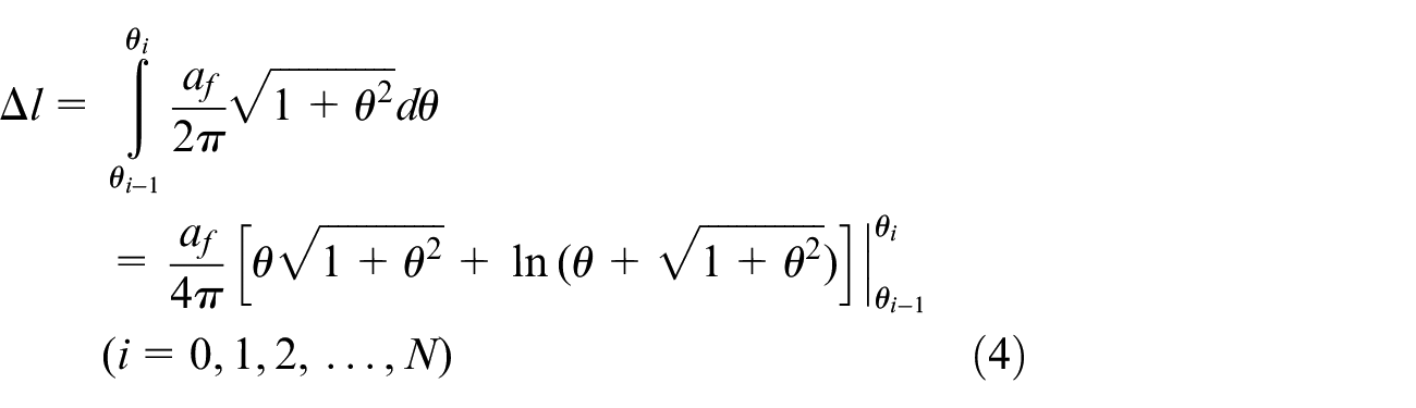
In STS turning process, the point on the tip of tool which contacts the machining surface is changing every time. The main objective of the machining process is to control the position of the tool relative to the workpiece. The NC program cannot control the movement of each axis with the tool contact point directly. It is necessary to compensate tool geometry on the basic of CCPs to generate CLPs. Assuming the tool rake angle is zero, tool geometry compensation means tool radius compensation. The schematic diagram of tool geometry is shown in Figure 4.

Figure 4.

Model of tool radius compensation: (a) 3D model, (b) plane model 1 and (c) plane model 2.

Figure 4(a) shows the condition of tool cutting workpiece’s surface. Where P is the CCP and curve CC is the intersection line between the XZ-plane and the complex surface. The vector n represents the normal vector of point P on the complex surface, vector n _p is the projection vector of vector n on the XZ-plane and vector t _p is the tangent vector of point P on the curve CC. The coordinate system of upper left corner in Figure 4(a) represents lathe coordinate system.

Figure 4(b) shows the XY-plane projection of Figure 4(a). The coordinate system shown in upper left corner in Figure 4(b) also represents lathe coordinate system. X_w-axis and Y_w-axis are the axes of workpiece coordinate. The mathematical expression of complex surfaces is based on this coordinate. Point O is the center point of workpiece and point P represents tool contact point. Line CC is same as in Figure 4(a), which is coincident with X-axis. C+ shows the direction of C-axis rotation and θ represents the angle between X_w-axis and line CC. The color shows the height of the surface.

Figure 4(c) shows the XZ-plane projection of Figure 4(a), and there are four different CLPs to explain the tool radius compensation. R_t is the radius of the tool. Curve CC is the trajectory connected by the CLPs on XZ-plane, and CL is the trajectory connected by the CLPs on XZ-plane. There are two methods to compensate the tool radius error, which are normal direction method and Z-direction method. The first step of the both methods is to get the equation of curve CC. Assume that the equation of the complex surface is z = f(x, y) and y = kx, where k = tanθ and θ is the angle between line CC and X-axis. So, equation z = f(x, y) can be transferred to z = φ(x, k). The equation of curve CC can be calculated as follows

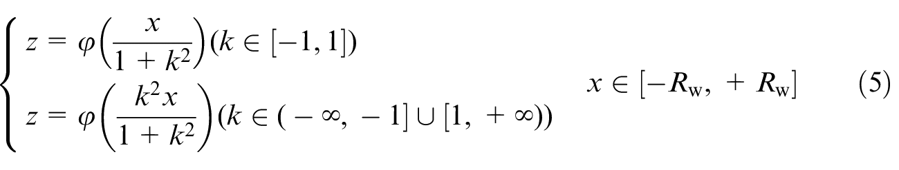
{\begin{matrix} z = φ (\frac{x}{1 + k^{2}}) (k \in [- 1, 1]) \\ z = φ (\frac{k^{2} x}{1 + k^{2}}) (k \in (- \infty, - 1] \cup [1, + \infty)) \end{matrix} x \in [- R_{w}, + R_{w}] (5)

(5)

where R_w represents the diameter of the workpiece. After getting the equation of curve CC, it is easy to calculate the unit tangent vector t _p1 to t _p4 and unit normal vector n _p1 to n _p4 of CCP P₁ to P₄.

The normal direction compensation includes Z-direction compensation and X-direction compensation, and the normal compensation length can be described as

Δ n_{i} = R_{t} \cdot n_{p i} (i = 1, 2, \dots, n)

(6)

where i is the number of X-axis feed ring, if X-axis feed velocity is a_f, n = R_w/a_f. The projected length of Δ n _i in X-axis and Z-axis is the compensation length of tool radius in X-direction and Z-direction, respectively.

After getting a series of tool location points, the piecewise cubic spline interpolation can be used to get the equation of curve CL. And then, the points L_i′ (i = 1, 2, …, n) which have the same z coordinates value can be obtained. And the points L_i′ (i = 1, 2, …, n) are the compensation points for Z-direction compensation. Cubic spline interpolation was used in Z-direction, which will cause interpolation error.

The two tool radius compensation methods have advantages and disadvantages when used in different applications. The mass of X-axis sliding platform is relatively large, so the dynamic characteristics of X-axis are not very accurate. When the Z-direction compensation is used, the X-direction compensation is zero and the X-axis moves at a constant speed, which can decrease the dynamic following error of X-axis and increase the machining accuracy. Normal compensation can be divided into X-axis compensation and Z-axis compensation. X-axis compensation makes X-axis to move with a slight oscillation and inconsistent speed, which can increase the dynamic following error. Therefore, if the dynamic characteristics of X-axis are not very accurate, Z-direction compensation is the better choice. Moreover, normal compensation is the simple calculation with less calculation error, so the normal compensation is the most suitable for the lathe which have good dynamic characteristics. Besides, equal arc length discretization and integrated method have a large amount of calculations, so normal compensation is more suitable in these conditions, because of its simple design and less calculation error.

Interpolation for STS

The IMAC can interpolate the machining trajectory according to the tool location generated above. The interpolation method supported by IMAC includes LINEAR, CIRTLE, SPLINE and PVT.¹⁹ According to the feature of STS, SPLINE and PVT can be used for the interpolation of the machining trajectory. SPLINE interpolation curve do not pass through the interpolation nodes, which will result in a large interpolation error, so PVT is chosen as the interpolation method.

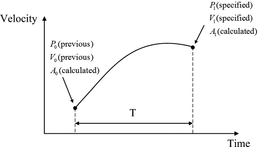
The essence of PVT mode is segment cubic Hermite interpolation, which can provide a method to direct control over the trajectory profile. As it is clear in Figure 5, in PVT mode, for each piece of movement, users should specify the end position or distance P₁, the end velocity V₁ and piece time T. From the specified parameters for the move piece, and the beginning position P₀ and velocity V₀, the IMAC computes the beginning acceleration A₀, end acceleration A₁ and the only third-order position trajectory path to meet the constraints.

Figure 5.

PVT interpolation diagram of servo axis segmentation.

In order to make servo axis pass exactly through the discrete CLPs with specified velocity and generate smooth trajectory, three entrance parameter algorithms of PVT were analyzed.

Area method

The scale coefficient c was introduced to represent velocity change rate in area method. The position increment could be expressed as¹

Δ P = P_{k + 1} - P_{k} = v_{k} h_{k} + c (v_{k + 1} - v_{k}) h_{k}

(7)

where $c \in [0, 1]$ .

For a specified time interval h_k, the endpoint velocity for each segment could be computed using equation (7). Different second-order velocity curves were combined to get an approximate velocity curve that can control the arbitrary contour path, which passes exactly through point P_k₊₁ with a continuous velocity.

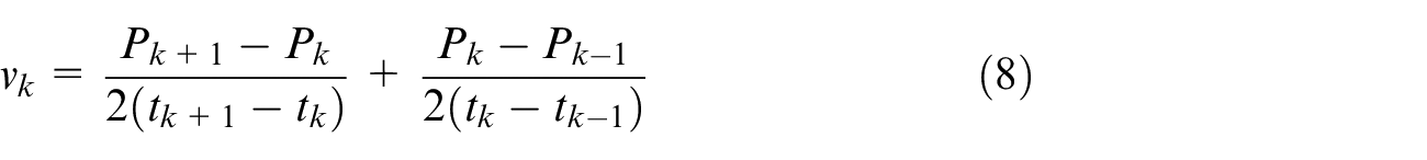
Three-point method

According to the above method, that is, (P_k₊₁, t_k₊₁), (P_k, t_k) and (P_k₋₁, t_k₋₁), the velocity at point k could be computed as¹⁸

v_{k} = \frac{P_{k + 1} - P_{k}}{2 (t_{k + 1} - t_{k})} + \frac{P_{k} - P_{k - 1}}{2 (t_{k} - t_{k - 1})}

(8)

Triangle rotary method

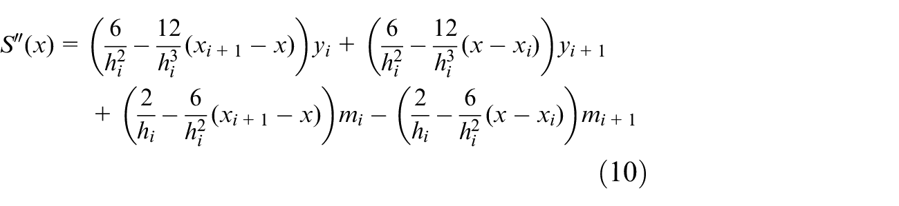
The same disadvantages of above two interpolation methods are they can only ensure the velocity of each cutting tool location point is continuous, but cannot guarantee the acceleration of each interpolation node is continuous, which will increase the interpolation error. In order to overcome above disadvantage, a new method referred to as triangle rotary method was put forward. This method can ensure that the equation of all axes is second-order continuous, that is, acceleration continuous. This transforms the segment Hermite interpolation to segment spline interpolation. First, considering the equation of segment cubic Hermite interpolation, the cubic Hermite interpolation polynomial for segment [x_i, x_i₊₁] can be described as²⁰

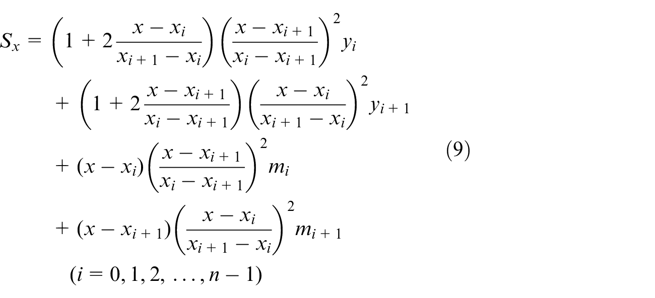
\begin{matrix} S_{x} = (1 + 2 \frac{x - x_{i}}{x_{i + 1} - x_{i}}) {(\frac{x - x_{i + 1}}{x_{i} - x_{i + 1}})}^{2} y_{i} \\ + (1 + 2 \frac{x - x_{i + 1}}{x_{i} - x_{i + 1}}) {(\frac{x - x_{i}}{x_{i + 1} - x_{i}})}^{2} y_{i + 1} \\ + (x - x_{i}) {(\frac{x - x_{i + 1}}{x_{i} - x_{i + 1}})}^{2} m_{i} \\ + (x - x_{i + 1}) {(\frac{x - x_{i}}{x_{i + 1} - x_{i}})}^{2} m_{i + 1} \\ (i = 0, 1, 2, \dots, n - 1) \end{matrix}

(9)

where i is the number of interpolation nodes, the total number of interpolation nodes is n + 1. m_i means the derivatives of x_i and y_i are the function value of x_i, and S_x is the interpolation function value of x for the segment [x_i, x_i₊₁].

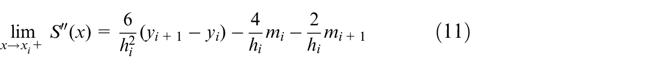
By calculating the two-order derivative of the above equation, the velocity of each segment could be expressed as

\begin{matrix} S ″ (x) = (\frac{6}{h_{i}^{2}} - \frac{12}{h_{i}^{3}} (x_{i + 1} - x)) y_{i} + (\frac{6}{h_{i}^{2}} - \frac{12}{h_{i}^{3}} (x - x_{i})) y_{i + 1} \\ + (\frac{2}{h_{i}} - \frac{6}{h_{i}^{2}} (x_{i + 1} - x)) m_{i} - (\frac{2}{h_{i}} - \frac{6}{h_{i}^{2}} (x - x_{i})) m_{i + 1} \end{matrix}

(10)

where h_i = x_i₊₁ − x_i; for x_i, the following formula can be obtained

lim_{x \to x_{i}^{+}} S ″ (x) = \frac{6}{h_{i}^{2}} (y_{i + 1} - y_{i}) - \frac{4}{h_{i}} m_{i} - \frac{2}{h_{i}} m_{i + 1}

(11)

lim_{x \to x_{i}^{-}} S ″ - (x) = \frac{- 6}{h_{i - 1}^{2}} (y_{i} - y_{i - 1}) + \frac{2}{h_{i - 1}} m_{i - 1} - \frac{4}{h_{i - 1}} m_{i}

(12)

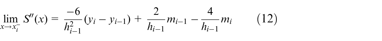
Letting

lim_{x \to x_{i}^{+}} S ″ (x) = lim_{x \to x_{i}^{-}} S ″ (x) (i = 1, 2, \dots, n - 1)

(13)

After consolidated and simplified the formulas (11)–(13), this formula was transformed to

λ_{i} m_{i - 1} + 2 m_{i} + μ_{i} m_{i + 1} = g_{i} (i = 2, 3, \dots, n - 1)

(14)

where

{\begin{matrix} λ_{i} = \frac{h_{i}}{h_{i} + h_{i + 1}} \\ μ_{i} = \frac{h_{i - 1}}{h_{i} + h_{i - 1}} = 1 - λ_{i} \\ g_{i} = 3 (λ_{i} \frac{y_{i} - y_{i - 1}}{h_{i - 1}} + μ_{i} \frac{y_{i + 1} - y_{i}}{h_{i}}) \end{matrix} (i = 1, 2, \dots, n - 1)

(15)

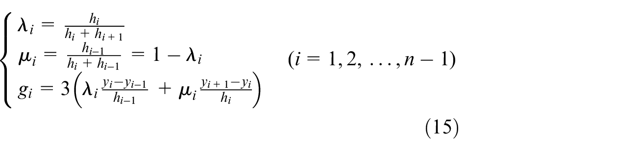
In total, there are m + 1 unknown numbers to solve, namely, m_i (i = 0, 1, 2, …, n), but only m − 1 equations were obtained above. So, introducing natural boundary conditions

{\begin{matrix} m_{0} = 0 \\ m_{n} = 0 \end{matrix}

(16)

The above m − 1 equations are transformed into matrix form as follows

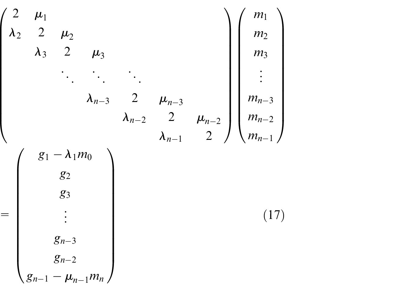
\begin{matrix} (\begin{matrix} 2 μ_{1} \\ λ_{2} 2 μ_{2} \\ λ_{3} 2 μ_{3} \\ ⋱ ⋱ ⋱ \\ λ_{n - 3} 2 μ_{n - 3} \\ λ_{n - 2} 2 μ_{n - 2} \\ λ_{n - 1} 2 \end{matrix}) (\begin{matrix} m_{1} \\ m_{2} \\ m_{3} \\ ⋮ \\ m_{n - 3} \\ m_{n - 2} \\ m_{n - 1} \end{matrix}) \\ = (\begin{matrix} g_{1} - λ_{1} m_{0} \\ g_{2} \\ g_{3} \\ ⋮ \\ g_{n - 3} \\ g_{n - 2} \\ g_{n - 1} - μ_{n - 1} m_{n} \end{matrix}) \end{matrix}

(17)

Equation (17) is a tri-diagonal matrix, and “chasing method” could be used to solve the m − 1 equations to get the entrance diameter of PVT method.

Machining simulation study

For STS turning, the C-axis rotates uniformly and the X-axis moves with a constant speed or only with slight oscillation. From this point of view, the overall TPG and its motion characteristics in Z-axis were simulated and analyzed during STS turning. The toric surface and sinusoidal surfaces are chosen as the simulation cases.

Toric surface

As it is shown in Figure 6, if the orthogonal arc (radius is R) rotates around the axis which is on the same plane with the orthogonal arc but do not through the circle center of the orthogonal arc (orthogonal arc radius R > the basic arc radius a), the complete toric surface can be achieved. Figure 6(a) represents the complete toric surface and Figure 6(b) represents toric surface spectacle lenses. The surface in Figure 6(b) corresponds to the surface in the red circle in Figure 6(a). Figure 7 shows a designed toric surface. Where X_wY_wZ_w represents the workpiece coordinate system axes, R is the radius of the orthogonal arc, a is the radius of basic arc, P is a point on the toric surface, r represents the distance between P and the origin of coordinates and θ represents the angle between the point P and positive direction of X_w-axis. The designed toric surface can be expressed as follows¹⁶

z = R + a - \sqrt{{(R + \sqrt{a^{2} - r^{2} \sin^{2} θ})}^{2} - r^{2} \cos^{2} θ}

(18)

Figure 6.

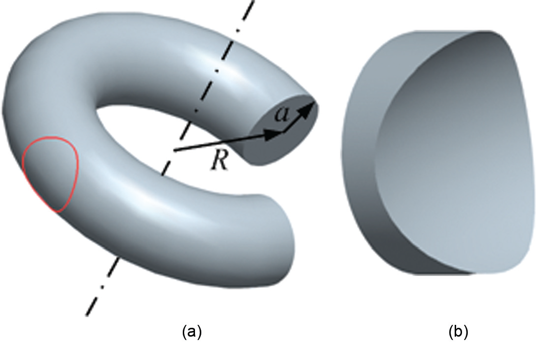
Diagram of toric surface: (a) complete toric surface and (b) toric surface spectacle lenses.

Figure 7.

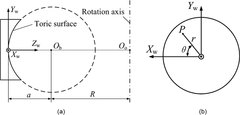
Designed toric surface: (a) Y_wZ_w plane and (b) X_wY_w plane.

The related parameters are defined in Table 1.

Table 1.

Parameters of machining toric surface simulation study.

Name of parameters	Radius of orthogonal arc, R (mm)	Radius of basic arc, a (mm)	Radius of workpiece, r (mm)	Discretization angle (°)
Parameter’s value	140	100	20	5
Name of parameters	Discretization arc length (mm)	The time between two nodes (ms)	Feed velocity (mm/s)	Tool radius (mm)
Parameter’s value	1	10	0.5	0.5

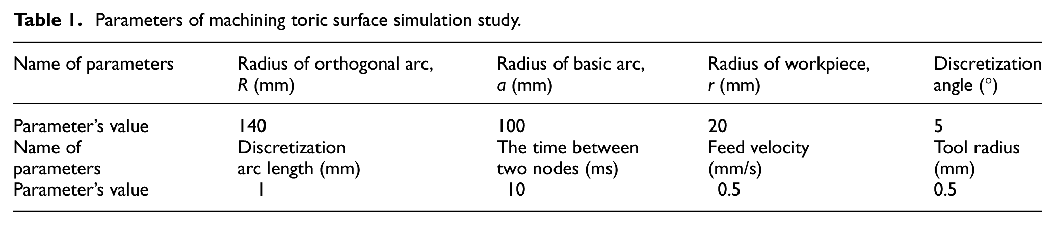
Figure 8 describes the designed toric surface and the tool path of toric surface discretized by integrated method. The Z-axis trajectory is demonstrated in Figure 9(a), which contains the CCPs’ trajectory and CLPs’ trajectory. As it is shown in Figure 9(b), discretization method was equal angle method, and the Z-axis and X-axis trajectories of outermost circle were different under different tool radius compensation. Figure 9(c) indicates that if the Z-direction compensation was chosen as the tool radius compensation method, the velocity of X-axis was constant when the equal angle method was used. And if the normal direction compensation was used, the X-axis moves with a slight oscillation, and the oscillation was not conducive to STS. Figure 10 shows the typical error variation rule for different discretization methods: the interpolation error was relatively large in outer circle of equal discretization and the interpolation error was relatively large in inner circle for equal arc length discretization. The integrated method can avoid the shortcomings of the above two kinds of discretization methods and get the minimum interpolation error.

Figure 8.

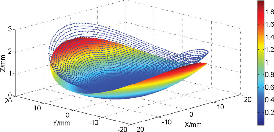
Designed surface and tool path of toric surface.

Figure 9.

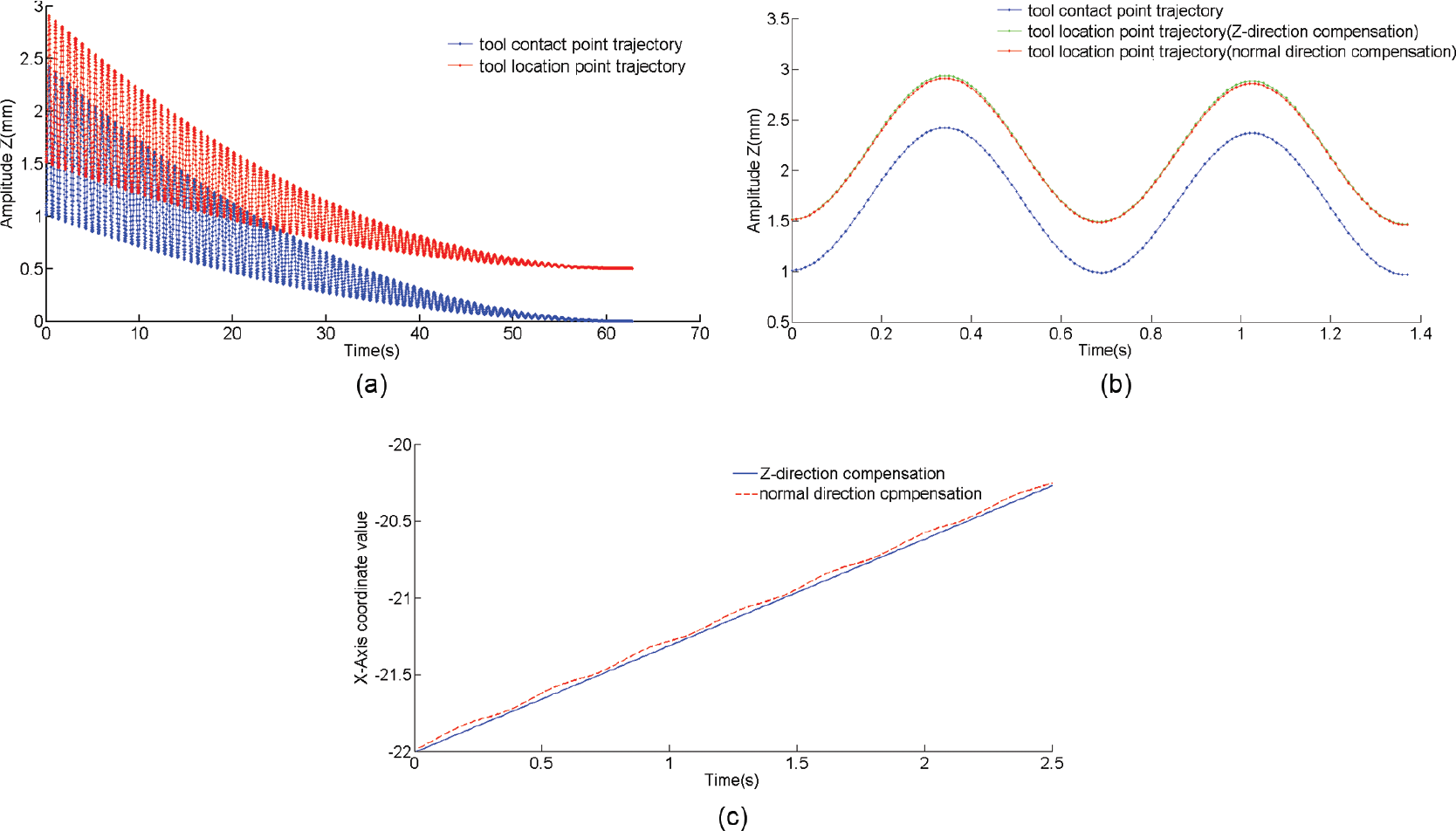
(a) Z-axis trajectory, (b) Z-axis trajectory of outmost circle and (c) X-axis trajectory of outermost three circles.

Figure 10.

The typical error variation rule for different discretization methods: (a) equal angle discretization method, (b)equal arc length discretization method and (c) integrated method.

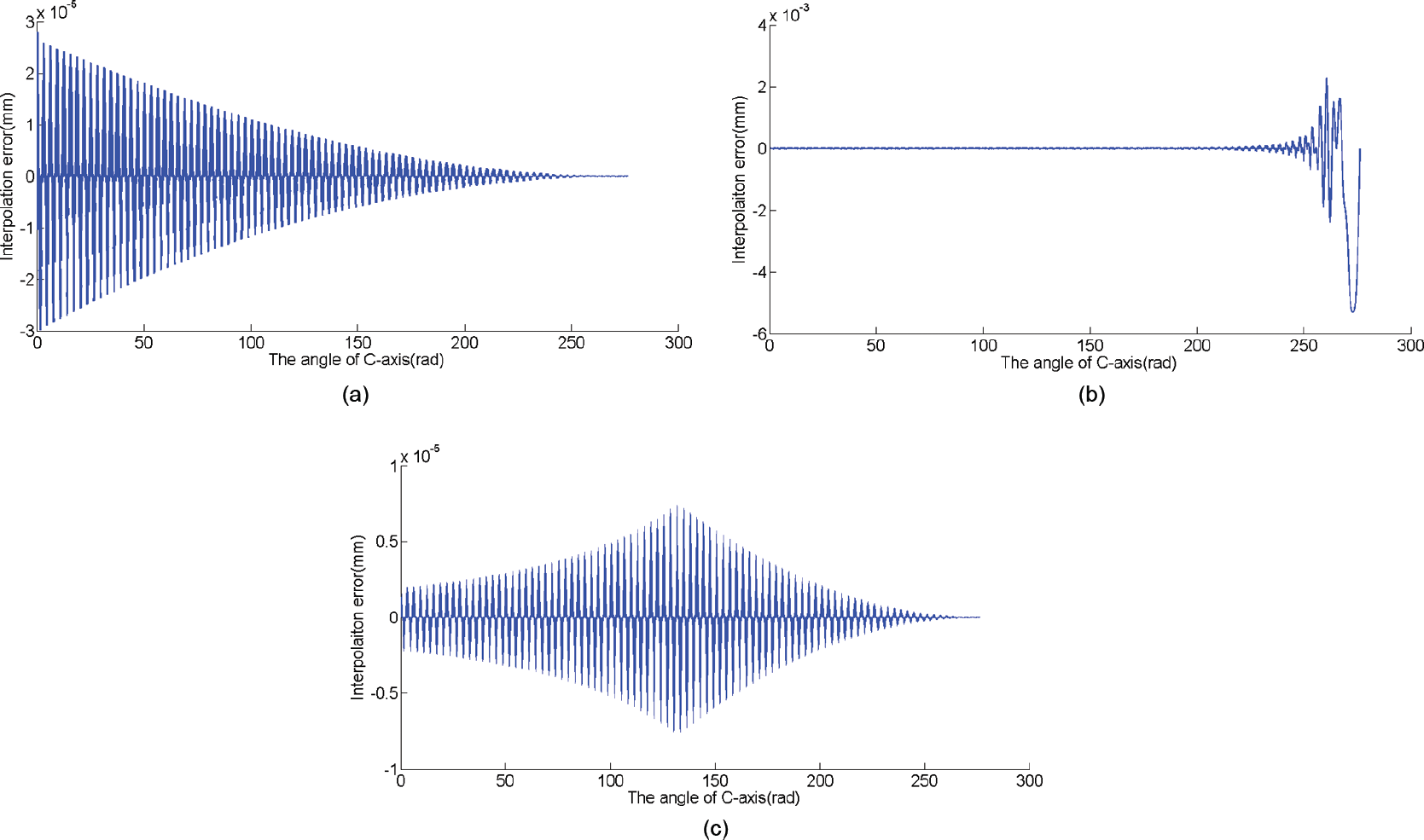
The velocity curve of Z-axis was different when using different methods to interpolation, as it is shown in Figure 11. Besides the area method (c = 1/2), other velocity curves were all very similar and smooth. Figure 12 shows the interpolation error of different algorithm for PVT; 1000 points from the “cutting in point” are analyzed. The maximum errors were summarized as follows: area method (c = 1/2) of 0.15 µm, (c = 2/3) of 0.3 µm, three-point method of 0.06 µm and triangle rotary method of 0.0015 µm. The simulation results indicated that triangle rotary method was the best algorithm, and three-point method was better than area method.

Figure 11.

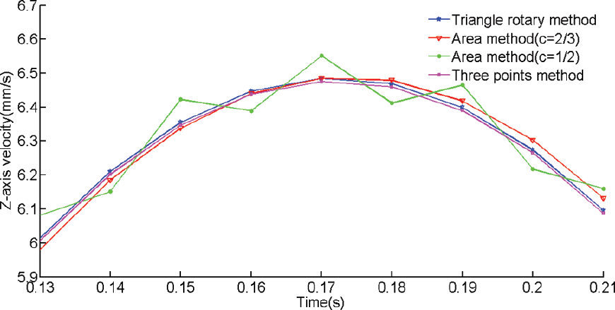
Z-axis velocity of different methods.

Figure 12.

The error of Z-axis for toric surface in different interpolation method: (a) area method, c = 1/2, (b) area method, c = 2/3, (c) three-point method and (d) triangle rotary method.

Sinusoidal array surface

The mathematical expression of sinusoidal array surface is given as follows¹

z = A \sin (\frac{2 π x}{ω}) \sin (\frac{2 π y}{ω})

(19)

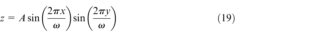
The related parameters are described in Table 2.

Table 2.

Parameters of machining sinusoidal array surface simulation study.

Name of parameters	Amplitude, A (mm)	Wave length, ω (mm)	Radius of workpiece, r (mm)	Discretization angle (°)
Parameter’s value	0.04	10	20	5
Name of parameters	Discretization arc length (mm)	The time between two nodes (ms)	Feed velocity (mm/s)	Tool radius (mm)
Parameter’s value	−	10	0.5	0.5

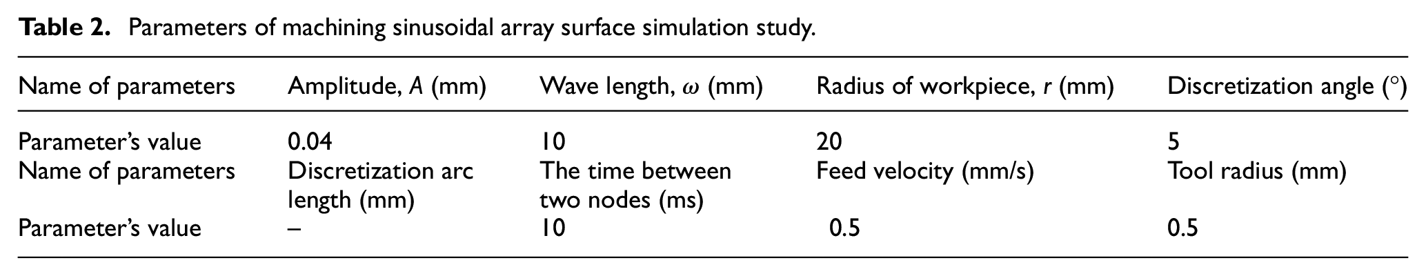
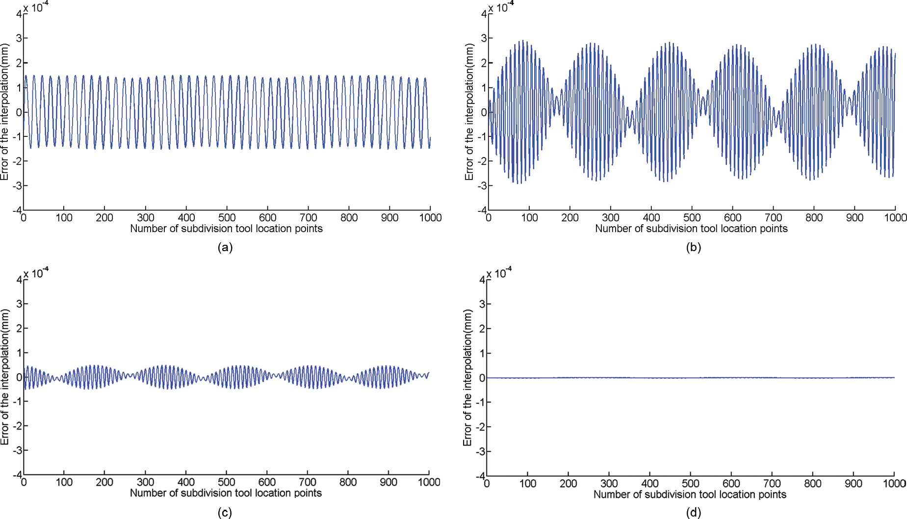
Figure 13 shows the designed surface and tool path of sinusoidal array surface discreted by equal angle method. Figure 14 shows the interpolation error of different algorithm for PVT; 1000 points from the “cutting in point” are analyzed. The maximum errors of these methods were area method (c = 1/2) of 1.5 µm, (c = 2/3) of 1.9 µm, three-point method of 1.8 µm and triangle rotary method of 0.37 µm. The simulation results indicated that triangle rotary method was the best algorithm, and three-point method was better than the area method.

Figure 13.

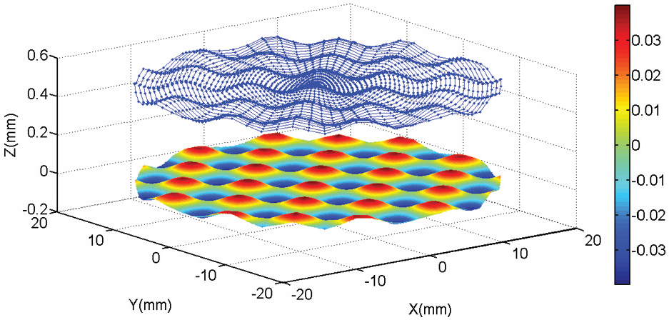
Designed surface and tool path of sinusoidal array surface.

Figure 14.

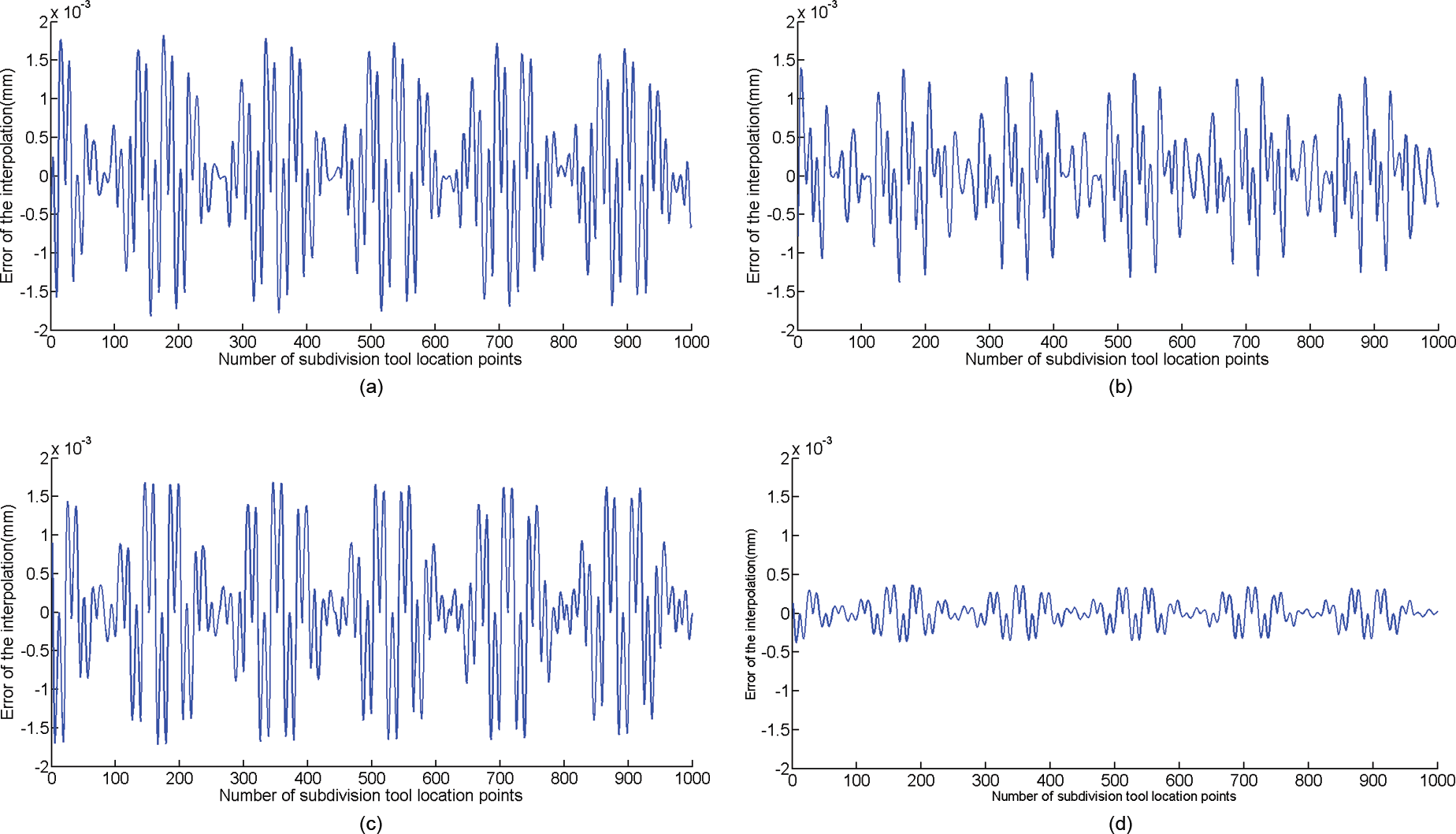
The error of Z-axis for sinusoidal array surface in different interpolation methods: (a) area method, c = 1/2, (b) area method, c = 2/3, (c) three-point method and (d) triangle rotary method.

Case study

According to the above analysis, the integrated method could be chosen as the discretization method when the workpiece’s size was large, and the equal angle method was a better discretization method for small workpieces. In order to ensure the velocity of the X-axis was constant and reduce following error, the Z-direction compensation was suitable for equal angle method discretization. For integrated method, the normal direction method was a better option, which was simple in calculation with less compensation error. The triangle rotary method was a better interpolation method than the area method and three-point method. So, the toric surface cases were machined by the two methods as given in Table 3.

Table 3.

Parameters of machining sinusoidal array surface simulation study.

	CLPs discretization method	Tool geometry compensation method	PVT interpolation method
Case A	Equal angle discretization	Z-direction	Triangle rotary method
Case B	Equal arc length discretization	Normal direction	Triangle rotary method

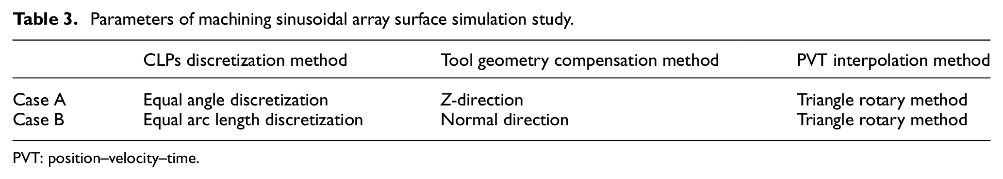
PVT: position–velocity–time.

The NC program for slow servo turning automatic generation program was written by C# language using the above-mentioned algorithm. For cases A and B, the material was polymeric methyl methacrylate (PMMA), the workpiece’s diameter was 40 mm, feed speed was 0.05 mm/r and the interpolation method was PVT interpolation method. For case A, the discretization angle was 5°. For case B, the discretization arc length was 1 mm and the discretization angle was 5°.

Figure 15 shows the machined workpieces. In order to evaluate the form accuracy of the machined toric surface workpieces, the toric surface was measured by MQ686 coordinate measuring machine. The form error is shown in Figure 16; the PV form error was about 0.0022 mm for case A and 0.0018 mm for case B, and root mean square (RMS) was about 0.0038 mm for the case A and 0.0034 mm for the case B. The surface roughness value was measured by a JB-4C instrument after dividing the machined lens surface into 12 aspects by the constant angle. The average value was used as the final roughness value, as shown in Figure 17, and the surface roughness of case A and case B was about 0.096 µm. The case study indicated that both the two TPG methods could be used to fabricate the complex surfaces by STS turning (Figures 16 and 17).

Figure 15.

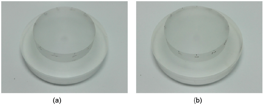
Machined result of toric surface: (a) case A and (b) case B.

Figure 16.

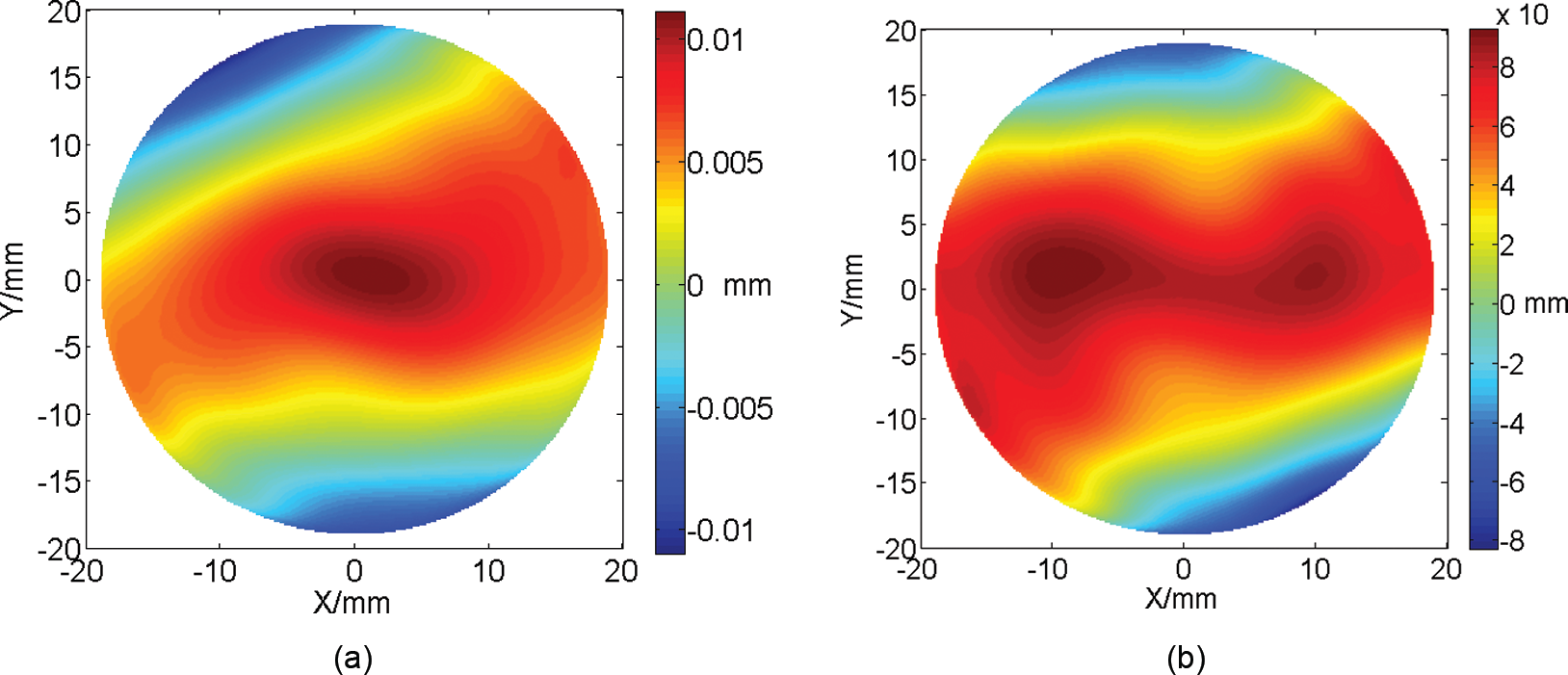
Plane form error of toric surface: (a) case A and (b) case B.

Figure 17.

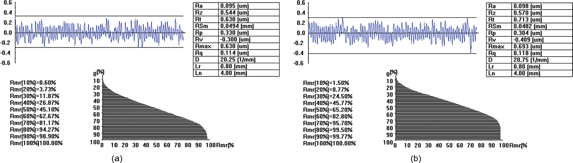
Surface roughness result of toric surface: (a) case A and (b) case B.

Conclusion

This article systematically studied the TPG for the STS turning of complex optical surfaces. Based on the result, the following conclusions can be drawn:

For large-size lenses, the integrated method could be chosen as the discretization method, and the equal angle method was a better discretization method for small workpieces. In order to ensure that the velocity of the X-axis was constant and reduce following error, the Z-direction compensation was suitable for equal angle discretization method. For equal arc length discretization method and integrated method, the normal direction method was a better option, which included simple calculation and zero interpolation error.

The PVT interpolation method can be used to machine optical complex surfaces; the core of the PVT interpolation was how to calculate the velocity (entrance parameters) of every contact tool point. A new interpolation method referred to as triangle rotary method was put forward and was compared with the area method and three-point method. The machining simulation of toric surface and sinusoidal array surface proved that the triangle rotary method can reduce the interpolation error obviously, which was the most feasible for the PVT interpolation.

For the large-sized workpieces, the recommended TPG methods were equal arc length cutting point discretization, normal tool radius compensation and triangle rotary method PVT interpolation. For small-sized workpiece, the recommended TPG methods were equal angle cutting point discretization, Z-direction tool radius compensation and triangle rotary method PVT interpolation. The experiment of the machining toric surfaces indicated that both the kinds of TPG methods could be used: the form error is about 0.002 mm and the surface roughness was about 0.096 µm in both methods.

Footnotes

Appendix 1 Declaration of conflicting interests

The author(s) declared no potential conflicts of interest with respect to the research, authorship and/or publication of this article.

Funding

The project was supported by Research and Innovation Project for College Graduates of Jiangsu Province (grant no. KYLX15_0565).

References

Guan

. Study on the technology of slow tool servo ultra-precision diamond turning for complex optical surface. PhD Thesis, National University of Defense Technology, Changsha, China, 2010.

Kwok

Cheung

Kong

. Analysis of surface generation in ultra-precision machining with a fast tool servo. Proc IMechE, Part B: J Engineering Manufacture 2009; 224: 1351–1367.

Tian

Yin

. Theoretical and experimental investigation on modeling of surface topography influenced by the tool-workpiece vibration in the cutting direction and feeding direction in single-point diamond turning. Int J Adv Manuf Tech. Epub ahead of print 27 January 2016. DOI: 10.1007/s00170-016-8363-4.

Zhou

Zhang

Huang

. Experimental study on the effects of feed rate and tool geometries on tool wear in diamond cutting of sinusoidal microstructured surfaces. Proc IMechE, Part B: J Engineering Manufacture 2010; 255: 172–183.

Neo

DWK

Kumar

Rahman

. CAx-technologies for hybrid fast tool/slow slide servo diamond turning of freeform surface. Proc IMechE, Part B: J Engineering Manufacture. Epub ahead of print 27 January 2016. DOI: 10.1177/0954405415625912.

Liu

Zhou

. A new tool path for optical freeform surface fast tool servo diamond turning. Proc IMechE, Part B: J Engineering Manufacture 2014; 228(12): 1721–1726.

Zhang

Fang

. Coordinate transformation machining of off-axis aspheric mirrors. Int J Adv Manuf Tech 2013; 67: 2217–2224.

Keong

Kumar

Rahman

. A novel method for layered tool path generation in the fast tool servo diamond turning of noncircular microstructural surfaces. Proc IMechE, Part B: J Engineering Manufacture 2012; 227: 210–219.

Kong

Cheung

. A theoretical and experimental investigation of design and slow tool servo machining of freeform progressive addition lenses (PALs) for optometric applications. Int J Adv Manuf Tech 2014; 72: 33–40.

10.

Tian

Yin

. Fast tool servo diamond turning of optical freeform surfaces for rear-view mirrors. Int J Adv Manuf Tech 2015; 80: 1759–1765.

11.

Zhou

Zhang

Chen

. Study on diamond cutting of nonrationally symmetric microstructured surfaces with fast tool servo. Mater Manuf Process 2010; 25: 488–494.

12.

Gong

Wang

Song

. Spiral tool path generation for diamond turning optical freeform surfaces of quasi-revolution. Comput Aided Design 2015; 59: 15–22.

13.

Hsu

Liu

Cheng

. Design, fabrication, and metrology of ultra-precision optical freeform surface for progressive addition lens with B-spline description. Int J Adv Manuf Tech 2012; 63: 225–233.

14.

Fang

Zhang

. Cylindrical coordinate machining of optical freeform surfaces. Opt Express 2008; 16: 7323–7329.

15.

Wang

. Research on the key technologies of slow tool servo turning for complex optical surface. PhD Thesis, Nanjing Agriculture University, Nanjing, China, 2014.

16.

. An accurate interpolator for FTS diamond turning of optical free-form surface. Int J Adv Manuf Tech 2014; 73: 635–638.

17.

Zhang

Fang

Wang

. Ultra-precision machining of sinusoidal surfaces using the cylindrical coordinate method. J Micromech Microeng 2009; 19: 1050–1055.

18.

Wang

. Tool path generation for slow tool servo turning of complex optical surfaces. Int J Adv Manuf Tech 2015; 79: 437–448.

19.

Turbo PMAC user manual, programmable multi axis controller. Delta Tau Data Systems, Inc., 2008, pp.278–294, http://www.deltatau.com

20.

Wang

. Numerical analysis. 5th ed.Beijing, China: Tsinghua University Press, 2008.

Tool path optimal design for slow tool servo turning of complex optical surface

Abstract

Keywords

Introduction

STS turning technology

TPG

CCP generation

Equal angle discretization method

Equal arc length method

Integrated discretization method

Cutting tool geometry compensation

Interpolation for STS

Area method

Three-point method

Triangle rotary method

Machining simulation study

Toric surface

Sinusoidal array surface

Case study

Conclusion

Footnotes

Appendix 1

Declaration of conflicting interests

Funding

References