An intelligent method to generate liaison graphs for truss structures

Abstract

Liaison graph is a necessary prerequisite of assembly sequence planning for mechanical products. Traditionally, it is generated via shape matching of joints among parts, but this strategy is invalid to truss structures because they lack patterns for shape matching. In this context, this article presents an intelligent method based on support vector machine to obtain liaison graphs of truss products automatically. This method defined three kinds of oriented bounding boxes to embody the relationships of the joints in truss structures. Based on them, a series of factors are deduced as training data for support vector machine. Furthermore, two algorithms are introduced to calculate oriented bounding boxes to facilitate the data extraction. By these processes, this method established the knowledge of joints and realized the intelligent construction of liaison graph without shape matching reasoning. To verify the effect of the method, an experimental implementation is presented. The results suggest that the proposed method could recognize most joint types and construct liaison graph automatically with sufficient sample training. The correct recognition rate is more than 85%. Comparing with back-propagation neural network, support vector machine is more accurate and stable in this case. As an alternative method, it could help the engineers to arrange the assembly plan for truss structures and other similar assemblies.

Introduction

To manufacture engineer, appropriate assembly sequence planning (ASP) could benefit product assembly in many aspects. ¹ However, ASP always demands liaison graph of products as a prerequisite ² which could not be generated directly from digital prototypes. Constructing such a liaison graph is a difficult, time-consuming work. To accelerate this process, many methods have been raised. However, these methods could not be used in truss structure effectively. Truss structures are important supporting bases which are widely used in mechanical products and architectures^3,4 and have been more and more complicated, which makes it difficult to plan assemblies. ⁵ In this context, this article presents an alternative method to recognize joint types in truss structures and then built liaison graphs consequently.

This article describes the method as follows. Section “Literature review” is a review of relative works. In section “The general liaison graph generating strategy for truss structure,” we analyze the characteristics of parts and joints and then extract a series of factors to embody these characteristics. Then, we introduce a machine learning method to bridge the joint types and the factors. To facilitate the calculation procedure, two approximate algorithms are presented in section “Fast algorithms for GB and RB solving.” In section “Case verification,” the whole method is tested and discussed with a case study.

Literature review

The ASP issue was raised in 1990 ⁶ and could be generated via computer soon. ⁷ However, as a necessary prerequisite for the ASP, the generation of liaison graph is not studied sufficiently. A common way is to model the liaison graph manually, such as constraint relationship and geometry relationship inputting method defined by Zhao et al. ⁸ and rule-based question–answer method proposed by Favi and Germani. ⁹ A manual liaison graph could express the assembly state precisely. But it is imaginable that this strategy might not be suitable to mass, complex assembly product. To generate liaison graphs from digital prototypes automatically, researchers have developed many methods which are mainly based on the shape matching reasoning. With surface relationships on the parts similar with b-rep representation, Case and Harun ¹⁰ define and extract assembly features to establish a liaison graph. Linn and Liu ¹¹ construct shape matching relationship via coplanar elements such as points, lines and surfaces. Sung et al. ¹² generate the liaison graph by detecting the adjacent surface features of two parts on the joint area. Kim et al. ¹³ propose their liaison graph generation method by detecting corresponding motion pair between parts. Hazarika et al. ¹⁴ generate liaison graph via predefined precedence relations existed in parts.

These studies have realized joint type detection with shape matching reasoning and then built liaison graphs consequently for many products with joints like screw connection or press fit because of their typical shape patterns. However, joint types of truss structures have different tolerance requirements and impact the assembly quality, respectively,^15–18 but do not have sufficient shape patterns. Figure 1 shows a digital truss model and the corresponding liaison graph. It could be seen that parts in these structures are only simple steel tubes and plate parts. The contact features between these parts are just flat surfaces. In these situations, the applicability of the aforementioned methods is reasonably limited and more effective method is demanded.

Figure 1.

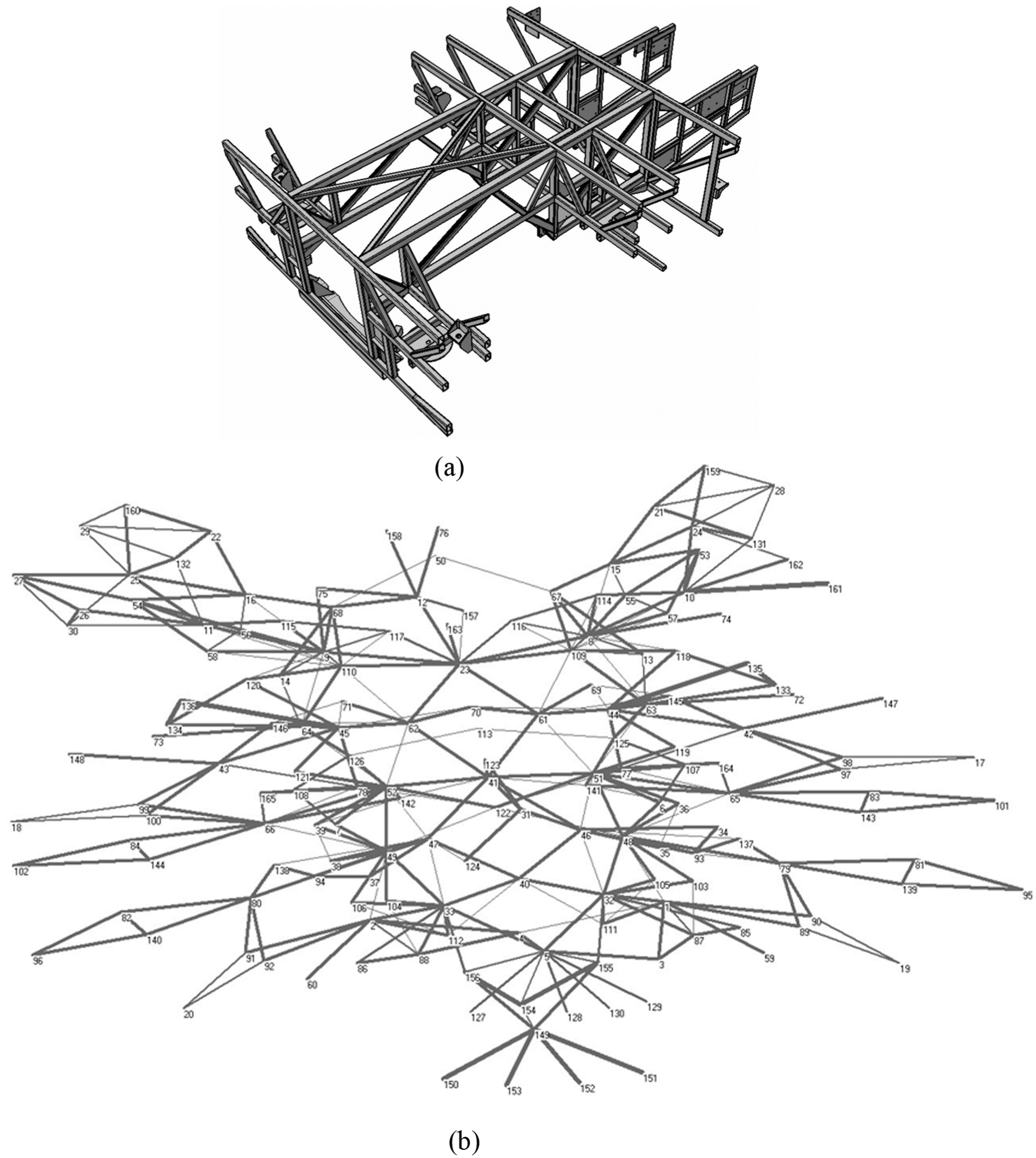
An example of truss structure: (a) digital model and (b) liaison graph.

Algorithm

The general liaison graph generating strategy for truss structure

The proposed method considers liaison graph generating as a knowledge discovery and data mining process. It means information contained in a digital model should be extracted and transformed into knowledge to detect joint types intelligently and consequently generate liaison graphs. Starting from this idea, this article chooses support vector machine (SVM) to carry out the joint type detection task. SVM is raised by Vapnik. ¹⁹ It is good at non-linear problem solving and was used to recognize milling conditions and so on in mechanical field. ²⁰ In our research, a software package called “LIBSVM” ²¹ is used to carry out the joint type recognition.

The performance of SVM depends on the quality of sample data which hinges on the typicality of the sample and the selection of factors. Noticing that simplicity is a common characteristic of parts in truss structure, this article chooses oriented bounding box (OBB) as a basic tool to evaluate the joint types of truss structures.

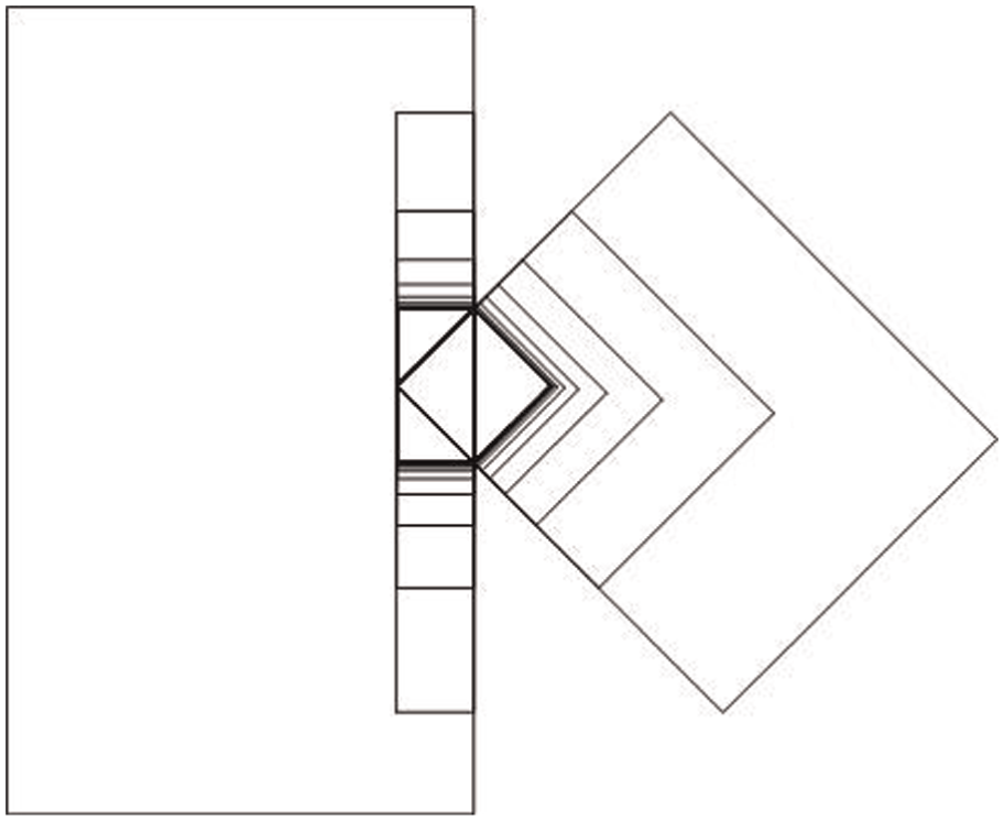
In fact, part pairs with similar correlations generally have same joint relationships. OBB could embody this kind of similarity in truss structure properly. To demonstrate each joint of a truss structure, three kinds of OBBs are defined. PB is defined as an OBB which contains a single part. GB is defined as an OBB which contains a pair of PBs. RB is defined as an OBB which contains the cross section of two PBs which belong to a GB. It is noticeable that the RB could degenerate to plane, line and point if some values of it are zeros. Figure 2 shows these three kinds of OBBs in 2D with a heavy line rectangle.

Figure 2.

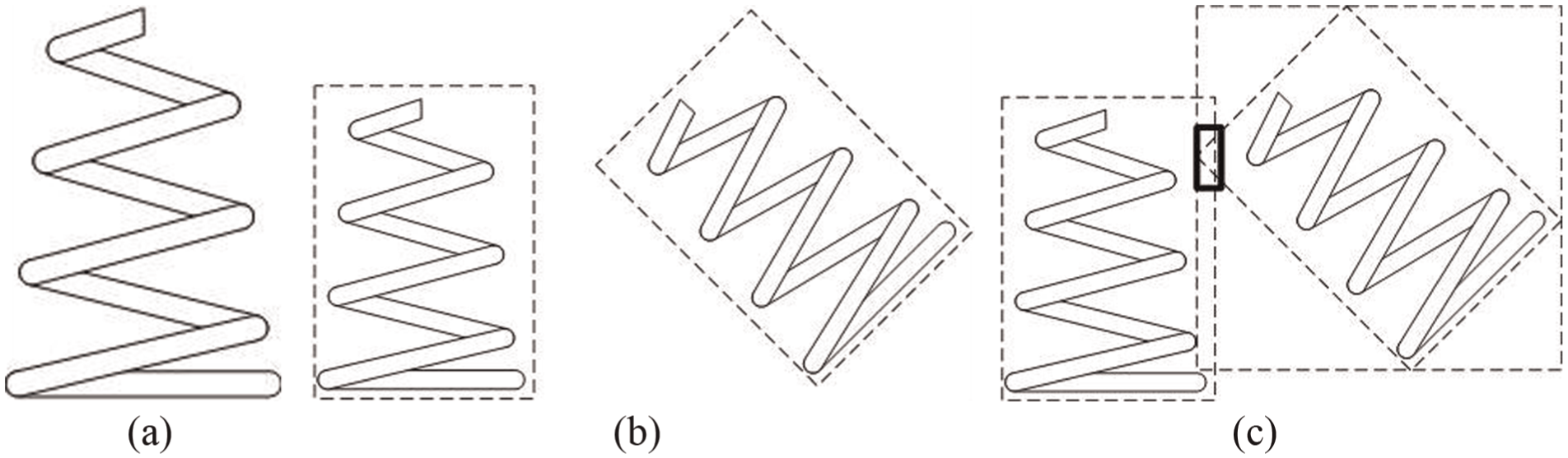
Three kinds of oriented bounding boxes are denoted as (a) PB, (b) GB and (c) RB.

The values of these OBBs are normalized to a vector combined with the scale information of these cuboids as equation (1), in which $a_1,a_2,a_3$ will be the expressed data for each OBB and $l,w,h$ is the corresponding length, width and height

$$\begin{array}{ccc}(a_1,\hfill & a_2,& a_3\end{array})=(\begin{array}{ccc}l,\hfill & w/l,& h/l)\end{array}$$

(1)

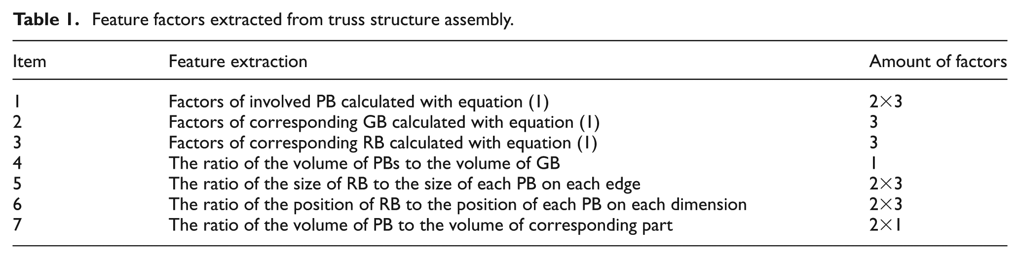
Starting from this basis, more data are deduced from these OBBs in specific rules to indicate the correlation between joint types and locating information of parts. These data are expressed as feature factors shown in Table 1. In addition, the ratio of the volume of PB to the volume of the corresponding part as another factor is added to demonstrate the compact degree of each part itself. The total number of factors is 27.

Table 1.

Feature factors extracted from truss structure assembly.

Item	Feature extraction	Amount of factors
1	Factors of involved PB calculated with equation (1)	2×3
2	Factors of corresponding GB calculated with equation (1)	3
3	Factors of corresponding RB calculated with equation (1)	3
4	The ratio of the volume of PBs to the volume of GB	1
5	The ratio of the size of RB to the size of each PB on each edge	2×3
6	The ratio of the position of RB to the position of each PB on each dimension	2×3
7	The ratio of the volume of PB to the volume of corresponding part	2×1

As an example of factor extraction, the joint relationship between part one and part two shown in Figure 3 could be interpreted into a feature factor vector. Assuming all three parts shown in Figure 3 are rectangle tubes whose sizes are 60 mm × 30 mm × 3 mm and the lengths of them are 300 mm. According to the items in Table 1, the corresponding feature factors should be (0.3, 0.2, 0.1, 0.3, 0.2, 0.1, 0.36, 0.83, 0.08, 0.6, 0.5, 0, 0.33, 0.2, 0, 1, 0, 1, 1, 1, 0.8, 0, 1, 0, 0, 0.29, 0.29).

Figure 3.

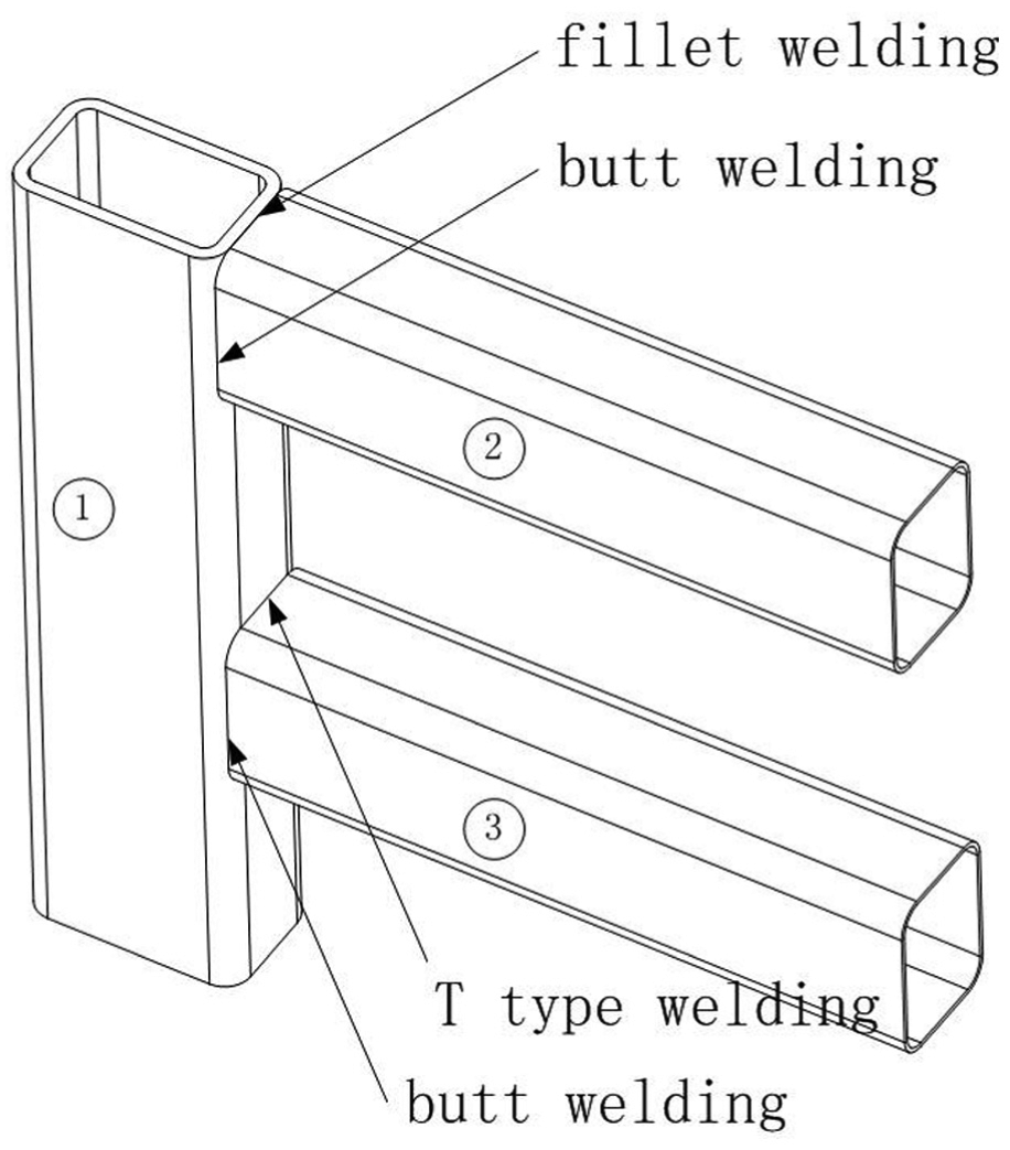
A simple truss structure.

The extracted factors are combined with joint type index to generate training data. It is noticeable that a joint could have more than one joint type. These types should be detected respectively. Besides that, we define a hybrid type as equation (2) to express this kind of type combination

$$\begin{array}{l}labe{l}_i={\displaystyle \sum _{k=1}^n{({\mathrm{num}}_{\max })}^k\times \delta {(i)}_k},\\ \delta {(i)}_k=\{\begin{array}{cc}t,& \mathrm{type}k\mathrm{exist}\\ 0,& \mathrm{type}k\mathrm{does\; not\; exist}\end{array}\end{array}$$

(2)

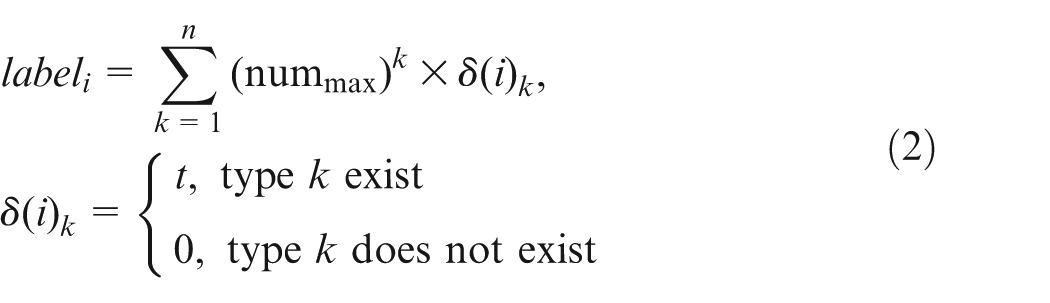
In this equation, i means the ith part pair and n is the total number of joint types. The num_max is a designated constant which must be bigger than the amount of members existed in any virtual joint. To any part pair i, $\delta (i{)}_k$ denotes the existence of the kth joint type. If this joint type does exist between this pair, t would be one in qualitative analysis or be the specific number in quantitative analysis.

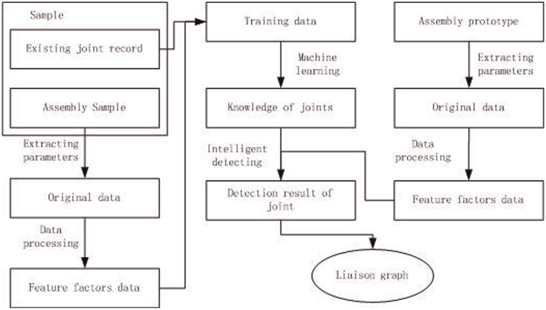
Apart from choosing the machine learning algorithm and extracting the feature factors, it is also necessary to establish a procedure for the intelligent liaison graph generation. The whole procedure could be seen in Figure 4: sample data of truss structure are obtained from corresponding digital models at first. Then, these data are used to construct feature factors listed in Table 1. Combining the feature factors with joint type labels remarked before will form the training data, with which the machine learning could establish knowledge of joint types. Finally, this knowledge is used to detect joint types existed in new truss products by analyzing feature factors extracted from them. With the detection results of joints, the liaison graph of corresponding products could be generated automatically.

Figure 4.

The flow of liaison graph generation procedure.

In this procedure, the most difficult task is to get the data of GB and RB based on the data obtained from the digital model of truss products. These data are used in each feature factor calculation offered in Table 1. For this reason, the following fast algorithms are introduced.

Fast algorithms for GB and RB solving

The most widely used algorithm to obtain size data of an OBB was raised by O’Rourke ²² in 1985. The complexity of this algorithm is $O(n^3)$ where n is the amount of vertexes. With this method, there are 16 vertexes that need to be considered for each GB. Moreover, an intersection computing must be carried out for each RB at first. Then, the similar operations should be done. This method is not efficient enough when the whole assembly is huge. To speed up the process, this article offered two approximation algorithms to obtain the GB and RB data based on PB information. For each GB, the two PBs of it were projected into mutual axis systems at first. The projections turned the problem into two axis-aligned bounding box (AABB) solving and one volume comparing tasks. The smaller one of the two AABBs would be considered as the approximate solution of the GB. For each RB, an iterative projecting process was carried out between the two PBs with their axis systems. In each iterative step, an axis-aligned intersecting box was calculated. The convergent result would be considered as the approximate solution of the RB. These two algorithms require only simple coordinate transformation and union or intersection computing. The specific mathematical description is given as follows.

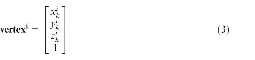
To obtain the data of a GB, each PB contained in it needs to be expressed with a matrix containing the homogeneous coordinates of its eight vertexes as equation (3). The superscript i is the serial number of part and the subscript k is the vertex sequence

$$\mathbf{verte}{\mathbf{x}}^{\mathbf{i}}=\left[\begin{array}{c}{x}_k^i\hfill \\ \multicolumn{1}{c}{y_k^i}\\ \multicolumn{1}{c}{z_k^i}\\ \multicolumn{1}{c}{1}\end{array}\right]$$

(3)

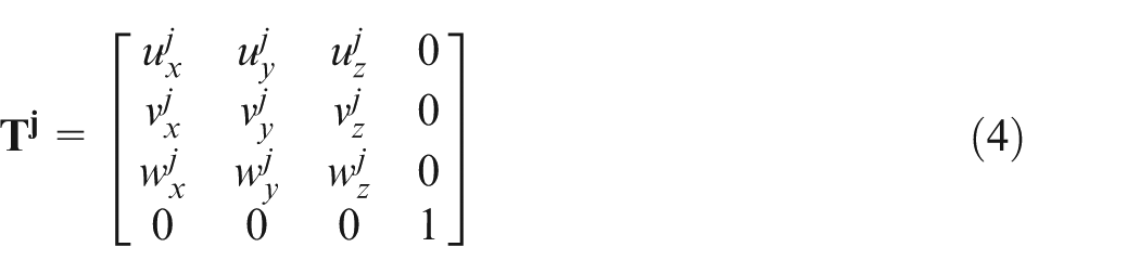
Then, establish a local axis system with the length, width and height dimension for each PB. The axis system could be expressed with the unit vectors shown as equation (4), in which the superscript j means the serial number of part and the subscripts x, y and z denote the global coordinate component of the vectors

$${\mathbf{T}}^{\mathbf{j}}=\left[\begin{array}{cccc}{u}_x^j\hfill & u_y^j& u_z^j& 0\\ \multicolumn{1}{c}{v_x^j}& v_y^j& v_z^j& 0\\ \multicolumn{1}{c}{w_x^j}& w_y^j& w_z^j& 0\\ \multicolumn{1}{c}{0}& 0& 0& 1\end{array}\right]$$

(4)

Left multiple equation (4) with equation (3) and choose the maximum and minimum value of each row of the result matrix. This step will get the projected value (data_min, data_max) of PB(i) on the axis system ${\mathbf{T}}^{\mathbf{j}}$ as equation (5), where the function max() and min(), respectively, gives the maximum and minimum value of each row of a matrix

$$\left[\mathbf{d}at{\mathbf{a}}_{{\mathbf{T}}_{\mathbf{j}},\mathbf{m}in}^{\mathbf{i}},\mathbf{d}at{\mathbf{a}}_{{\mathbf{T}}_{\mathbf{j}},\mathbf{m}ax}^{\mathbf{i}}\right]=\left[\min ({\mathbf{T}}^{\mathbf{j}}\ast \mathbf{v}erte{\mathbf{x}}^{\mathbf{i}}),\max ({\mathbf{T}}^{\mathbf{j}}\ast \mathbf{v}erte{\mathbf{x}}^{\mathbf{i}})\right]$$

(5)

Combining all the results of equation (5) for each i could generate a cuboid aligned with ${\mathbf{T}}^{\mathbf{j}}$ . The cuboid could be marked as $[\mathbf{dat}{\mathbf{a}}_{{\mathbf{T}}_{\mathbf{j}}}]$ as equation (6), where the function max_i() and min_i(), respectively, gives the maximum and minimum value of each row of the matrix of the whole range of i

$$\left[\mathbf{dat}{\mathbf{a}}_{\mathbf{Tj}}\right]={max}_i({\mathbf{data}}_{\mathbf{Tj}\mathbf{,}\mathbf{max}}^{\mathbf{i}})-{min}_i({\mathbf{data}}_{\mathbf{Tj}\mathbf{,}\mathbf{min}}^{\mathbf{i}})$$

(6)

Then, choose the one which has a smaller volume from axis system ${\mathbf{T}}^{\mathbf{j}}$ for each j. This step could be expressed as equation (7) in which f_{min_volume} is a function comparing the volume of the cuboid computed with equation (6)

$$\mathbf{dat}{\mathbf{a}}_{\mathbf{obb}}=f_{min\_\mathrm{volume}}({\mathbf{data}}_{\mathbf{Tj}}^{\mathbf{i}})$$

(7)

In this way, the amount of calculation is less than 10% of O’Rourke’s algorithm because only coordinate transformations are calculated twice. To verify the effectiveness of this approximation, a Monte Carlo test was carried out. At first, two rectangles contacted with each other was generated with random dimensions and contacting position in a 2D plane at one time. Then, the area of GB comprising these two rectangles is calculated with the approximate method and O’Rourke’s algorithm. Figure 5(a) shows an example of calculated results. This calculation is carried out 1000 times and at each time the ratio between the areas generated from the two methods are calculated. Figure 5(b) shows a sample of these results. It shows that in most situations, the approximate method was as good as O’Rourke’s method. The mean value of the ratio is 0.97 and the deviation is 0.0031. It suggests that the proposed method is feasible.

Figure 5.

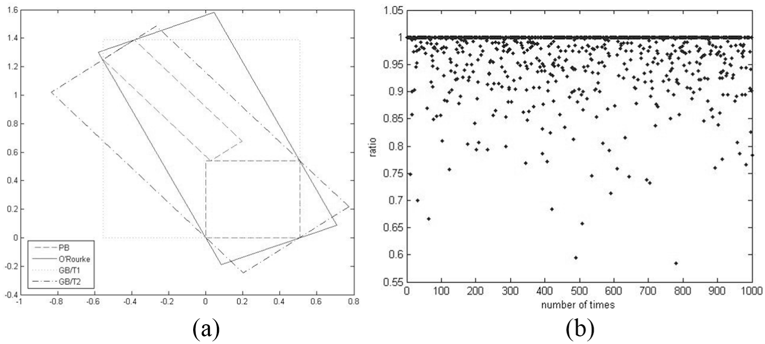
(a) Two different methods to calculate the area of GB and (b) the ratios between the results of O’Rourke’s method and the proposed approach in a Monte Carlo test.

To obtain the data of an RB, a similar projected cuboid $[{\mathbf{data}}_{\mathbf{Tj}}^{\prime }]$ aligned with each axis system could be calculated based on the same idea as shown in equation (8)

$$\left[{\mathbf{data}}_{\mathbf{Tj}}^{\prime }\right]=\mathrm{mi}{\mathrm{n}}_i({\mathbf{data}}_{\mathbf{Tj}\mathbf{,}\mathbf{max}}^{\mathbf{i}})-\mathrm{ma}{\mathrm{x}}_i({\mathbf{data}}_{\mathbf{Tj}\mathbf{,}\mathbf{min}}^{\mathbf{i}})$$

(8)

Then, an iterative algorithm is used to get a more rigorous result. At first $({\mathbf{data}}_{\mathbf{Tj}}^{\prime }{)}_1$ is calculated in any ${\mathbf{T}}^{\mathbf{j}}$ with equation (8). Then, construct a new cuboid with the result and express it with vertexes as ${\mathbf{vertex}}_1^{\mathbf{j}}({\mathbf{data}}_{\mathbf{Tj}}^{\prime })$ . Let it be the new $P{B}^j$ to replace the original $\mathrm{verte}{x}^j$ and calculate $({\mathbf{data}}_{\mathbf{Tj}\prime }^{\prime }{)}_1$ in another axis system ${\mathbf{T}}^{\mathbf{j}\mathbf{\prime }}$ with equation (8). Consequently, the kth iterative equation on axis system ${\mathbf{T}}^{\mathbf{j}}$ should be as follows

$$\begin{array}{c}\multicolumn{1}{c}{\left[{({\mathbf{data}}_{\mathbf{Tj}}^{\prime })}_k\right]=min((({\mathbf{data}}_{\mathbf{Tj}}^{\prime }{)}_{k-1}{)}_{\mathrm{Tj},max},(({\mathbf{data}}_{\mathbf{Tj}\prime }^{\prime }{)}_{k-1}{)}_{\mathrm{Tj},max})}\\ \multicolumn{1}{c}{-max((({\mathbf{data}}_{\mathbf{Tj}}^{\prime }{)}_{k-1}{)}_{\mathrm{Tj},min},(({\mathbf{data}}_{\mathbf{Tj}\prime }^{\prime }{)}_{k-1}{)}_{\mathrm{Tj},min})}\end{array}$$

(9)

To terminate the iteration, a threshold such as a specific k or the shrink ratio of the result should be given. Generally, k is less than 15. An example of the iterative method is shown in 2D in Figure 6. This method involves only matrix multiplication. The amount of calculation is less than 75% of O’Rourke’s algorithm. More important, the cross section could be estimated without complex intersecting calculation. It would be convenient to obtain the data of GB and RB with the proposed two approximate algorithms.

Figure 6.

An example of the iterative method proposed to calculate an RB.

Case verification

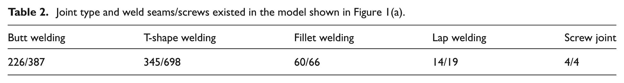
We selected the truss structure shown in Figure 1(a) to verify the joint type recognition performance of the method proposed by this article. The truss structure shown in Figure 1(a) comprises 165 parts and 364 joints existed between these parts. The parts are made of steel rectangle tubes and steel rolling plates. Most joints are welding shown in Figure 3. Table 2 shows the amount of joints/seams (screws) existed in this structure.

Table 2.

Joint type and weld seams/screws existed in the model shown in Figure 1(a).

Butt welding	T-shape welding	Fillet welding	Lap welding	Screw joint
226/387	345/698	60/66	14/19	4/4

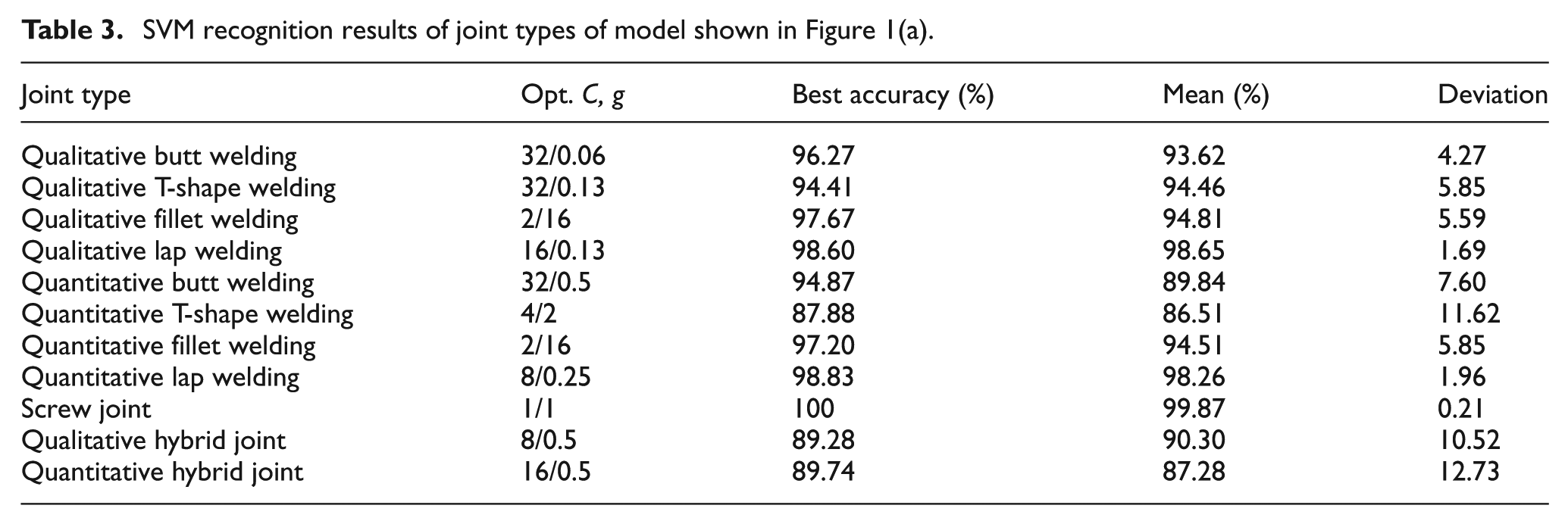
It could be seen that joint types are mainly defined by welding methods while screw connections are used too. Apart from the recognition of each single joint type, a qualitative hybrid joint type and a quantitative hybrid joint type based on equation (2) are defined. The num_max in equation (2) is specified as 10 in this case.

Extracting feature factors from the digital model demands several steps. At first, the digital model was built in CATIA. Then, several VBA programs inside the CATIA environment were written to extract the PB data and volume data into an EXCEL sheet. Based on the original PB data, a MATLAB program is used to calculate the corresponding GB and RB data with the approximate algorithms proposed in this article and then consequently output the feature factors according to the items listed in Table 1.

Combining the joint type information with the feature factors, the training data are generated. With the training data, the SVM software could build knowledge of truss structure joint types. This process was carried out with LIBSVM under the environment of MATLAB. The kernel function of LIBSVM is optional. In this case, the radial base function (RBF) was chosen. To acquire the best performance, the parameters of RBF including C and g were optimized with the net method. With the optimistic parameters, 70% of the sample data was chosen randomly as the training data to predict the remaining 30% data. This random process was carried out for 1000 times to confirm the accuracy and deviation of the prediction.

According to the above method, the LIBSVM was trained successively with the joint types shown in Table 2. The recognition results are listed in Table 3. It should be point out that there are only four screw joints existed in this truss structure and the state of them is the same. For this reason, the qualitative recognition and the quantitative recognition of screw joints in this case are identical.

Table 3.

SVM recognition results of joint types of model shown in Figure 1(a).

Joint type	Opt. C, g	Best accuracy (%)	Mean (%)	Deviation
Qualitative butt welding	32/0.06	96.27	93.62	4.27
Qualitative T-shape welding	32/0.13	94.41	94.46	5.85
Qualitative fillet welding	2/16	97.67	94.81	5.59
Qualitative lap welding	16/0.13	98.60	98.65	1.69
Quantitative butt welding	32/0.5	94.87	89.84	7.60
Quantitative T-shape welding	4/2	87.88	86.51	11.62
Quantitative fillet welding	2/16	97.20	94.51	5.85
Quantitative lap welding	8/0.25	98.83	98.26	1.96
Screw joint	1/1	100	99.87	0.21
Qualitative hybrid joint	8/0.5	89.28	90.30	10.52
Quantitative hybrid joint	16/0.5	89.74	87.28	12.73

The results demonstrated the feasibility and effectiveness of the proposed intelligent recognition method. For comparison, the feature factors were also used to train a back-propagation (BP) neural network in the MATLAB environment. The recognizing results of BP neural network are shown beside the results of SVM in Figure 7 where Figure 7(a) shows the accuracies of the two methods and Figure 7(b) shows the deviations. It could be seen that the proposed method had a better recognition capability and stable performance than BP neural network in this case. To demonstrate the importance of the feature factors defined in this article, SVM recognizing results based on original PB data are shown too in Figure 7(a). It is clear that the results based on original data have lower performance compared with the proposed method. Time-consuming of the whole process is shown in Figure 7(c). It shows that the proposed algorithm for OBB is significantly quicker than O’Rourke’s. Meanwhile, the SVM algorithm is also quicker than BP method too. The whole time-consuming is less than 7 min, which suggests the practicability of this method.

Figure 7.

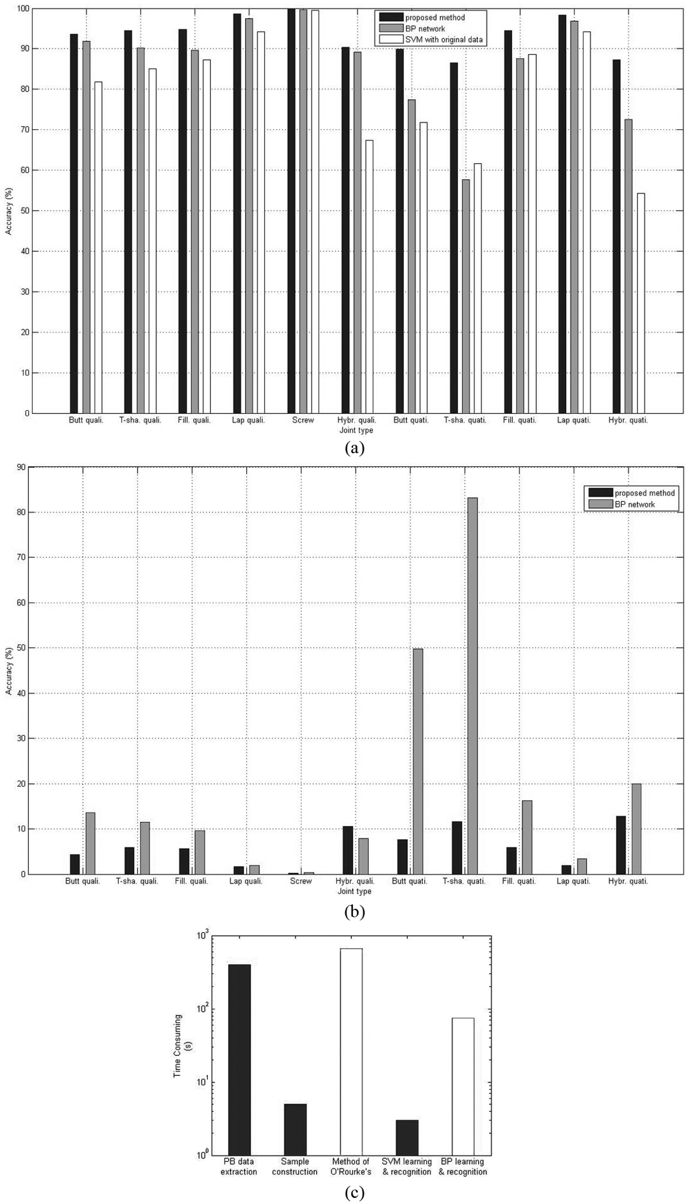
Two intelligent recognizing methods on (a) prediction accuracy and (b) corresponding deviation are compared. (a) A comparison between defined feature factors and original data on prediction accuracy are also presented. (c) Time-consuming of the whole process is also calculated.

In this case, most joint relationships were recognized properly by the proposed method. However, there still existed several part pairs which cannot be recognized accurately. It is believed that the false recognition might derive from the following reasons. The first reason is that the samples of some joint relationships are too small. As an example, only two instances of the joint type shown in Figure 8(a) exist in the whole structure. The scarcity of the sample makes it difficult to learn the joint relationship. The second reason is that some joint types are not significant enough to be defined to a specific category. As shown in Figure 8(b), the denoted joint could be both considered as butt welding or T-shape welding. This kind of ambiguity might cause the failure. The final reason is that some connections are changed manually by the engineer. For example, the joint denoted in Figure 8(c) was canceled because they were too short, but the SVM still regarded it as a T-shape welding.

Figure 8.

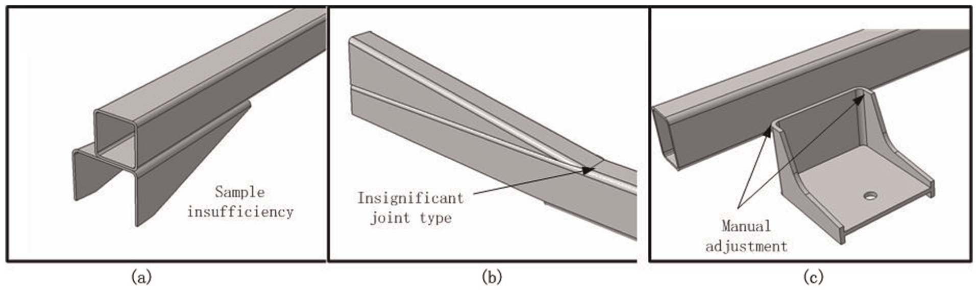
Reasons of mistake recognizing include (a) scarcity of sample, (b) ambiguity of joint types and (c) manual change.

To some extent, these faults could be corrected. Increasing the sample size can enhance the capability of SVM to recognize the infrequent joint relationship. Sufficient samples also benefit the pattern building for some manually adjusted cases if the modification is regular though irregular cases must be adjusted manually. Finally, more effective learning strategy or more representative type definition might need for the insignificant joints. However, the insignificant types are rare in our case. For this reason, it is believed that the proposed method is effective and practical.

Another noticeable fact is that five mistakes were not made by machine learning but engineers. Wrong labels were given carelessly. It suggests that this method could be used to prevent human errors too.

Finally, the trained program is used to recognize joint types of a raw truss model. The correct recognition rate about this model is still more than 85%. Figure 9 shows the computer-aided design (CAD) model and corresponding liaison graph generated with Pajek.

Figure 9.

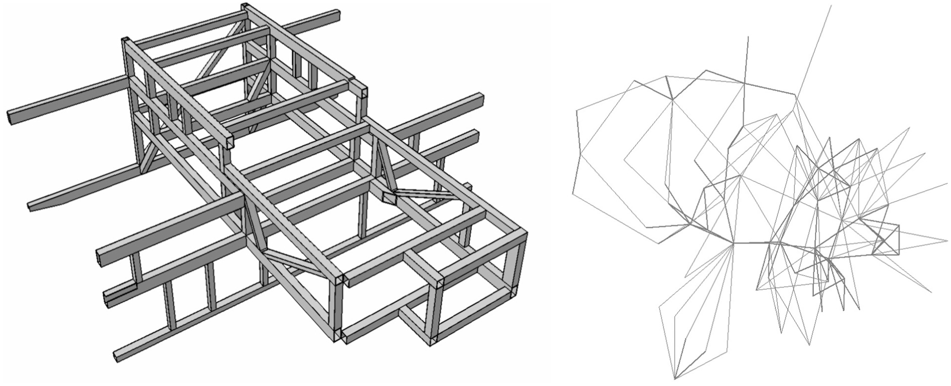
A raw model could be recognized properly and then be transformed to a liaison graph.

Conclusion

An intelligent method is presented to generate liaison graphs for truss structures automatically. A series of feature factors are proposed with two approximate algorithms to form training data. Then, a SVM program is used to learn the training data and achieve the knowledge of joint types. A case study is carried out to verify the effectiveness and practicality of the method. This study draws the following conclusions:

1. The proposed method could recognize most joint types properly in our case. For this reason, it could be used as an alternative approach to replace shape matching method when assemblies do not have sufficient shape patterns.

2. Comparing with another intelligent method, the SVM is more accurate and more stable in joint type recognition. Meanwhile, the time-consuming is acceptable. It suggests the SVM would be a rational choice in this field.

3. By comparing with the performance of the SVM based on original PB data, the effectiveness of proposed feature factors is verified that it could enhance the capability of machine learning.

4. The two approximate algorithms presented in section “Fast algorithms for GB and RB solving” work correctly. Comparing with traditional method, it could obtain the OBB data more quickly. For this reason, they shorten the whole solving time significantly. The acceptable time-consuming guarantee the practicality of the proposed method.

The subsequent working would be finding more appropriate learning methods and more representative features to make the method more practical.