Sage Journals: Discover world-class research

Abstract

Assembly optimisation activities that involve assembly sequence planning and assembly line balancing have been extensively studied because of the importance of optimal assembly efficiency to manufacturing competitiveness. Numerous research works in assembly sequence planning and assembly line balancing mainly focus on developing algorithms to solve problems and to optimise assembly sequence planning and assembly line balancing. However, there is a scarcity in works that focus on developing problems to test these algorithms. In optimisation algorithm development, testing algorithms by a broad range of test problems is crucial to identify their strengths and weaknesses. This article proposes a generator of assembly sequence planning and assembly line balancing test problems with tuneable complexity levels. Experiments confirm that the selected combination of input attributes does control the generated assembly sequence planning and assembly line balancing problem complexity, and also that the generated problems can be used to identify the suitability of a given algorithm to problem types.

Keywords

Assembly sequence planning assembly line balancing test problem generator

Introduction

In manufacturing, assembly optimisation involves bringing and joining parts and/or subassemblies together to make the process as efficient as possible. Assembly sequence planning (ASP) and assembly line balancing (ALB) are classified among major topics in assembly optimisation because both are directly related to assembly efficiency.^1,2 Recently, researchers have discovered benefits of solving and optimising ASP and ALB problems together,^3,4 leading to increased research focus on testing new or improved algorithms that operate on these combined problems. In order to assess the performance of new or improved algorithms and to compare them with existing algorithms, a wide range of test problems are required. In ASP and ALB optimisation works that focus on algorithm development or improvement, researchers have used two approaches to test algorithm performance. One approach is to test the algorithms using specific case studies.^5,6 Another acknowledged approach is to adopt the test problems that are frequently used in literature.^7,8 These approaches lack generality because there has been no investigation into the fit of algorithms to problem types. Algorithms have not been tested with a wide range of problem types.

The most frequently used test problem in ASP is an assembly of a transmission-type part with eleven components, presented by De Fazio and Whitney.⁹ This problem has been presented in many articles, such as Chen and Liu,¹⁰ Smith and Liu¹¹ and Wang et al.,¹² to evaluate algorithm performance. Other than this widely used problem example, most ASP test problems found in literature have only been used within the same research group. There is thus no accepted standard ASP test problem for evaluating algorithm performance. On the other hand, in ALB optimisation, development of test problems was started in 1960s, resulting in many that have been developed and collected by different researchers. These problems vary in task size from eight to 297 tasks. The famous ALB problems, such as the eight-tasks by Bowman, 45 tasks by Kilbridge and Wester, 70 tasks by Tonge, 111 tasks by Arcus and 297 tasks by Scholl, are still being used until today to evaluate algorithm performance for line balancing problems.¹³

Although these few benchmark ASP and ALB problems are available for comparing algorithm performance, there is no standard test problem set that covers a wide variety of problem difficulties, especially to test the combined ASP and ALB optimisation. Not only is this important for enhancing the researchers’ understanding of their algorithm, it will also help users in selecting which algorithm is more appropriate to their requirements. In order to facilitate such experimentation, a set of problems with a controllable complexity level is needed. One way to address this is to devise a test problem generator (TPG) with tuneable difficulty level that can systematically generate a set of test problems with a desired mix of complexity levels.

This article proposes a TPG with a tuneable complexity level for combined ASP and ALB problems. ‘TPG for ASP and ALB’ explains the requirements and specifications for the proposed TPG. ‘TPG development’ will explain the methodology of the TPG development, which is divided into graph and data generation methodology. Then, ‘Experimental design’ describes the experimental design to test the proposed TPG for ASP and ALB. ‘Results and discussion’ presents and discusses the experimental results in this work. Finally, we present the authors’ conclusions on the proposed TPG according to experimental results.

TPG for ASP and ALB

In the mathematical optimisation community, the importance of TPGs is widely appreciated. Although algorithm development is important, any new algorithm should ideally be tested with a wide range of problem types before making any conclusion on their usefulness.¹⁴ Most of ASP and ALB works focus on proposing and demonstrating algorithm performance on specific ASP and/or ALB problems. There is a lack of investigation into testing and validating the performance of algorithms on wider classes of problems.

A TPG will be useful to provide a wide range of ASP and ALB problems with differing characteristics and difficulties. In many cases, the problem difficulty is only determined by the size of the problem. While this is correct in certain cases, this overlooks the influence of many other attributes on problem difficulty. Additionally, TPGs will also be useful to identify which algorithm may be more suitable for a given type of problem. This knowledge is very important to help users to choose the right algorithm, and also for researchers to identify opportunities for further improvement in a particular algorithm.

To provide the mentioned benefits, the TPG must satisfy the following requirements.

Representation. The problems are generated on the basis of assembly task and represented using a precedence graph. This was the common way to represent task-based assembly problems in earlier works.²

Output. The TPG is expected to produce precedence graphs that represent task-based assembly problems. Besides that, the TPG must also be able to generate assembly data, which consists of assembly direction and tool for ASP and assembly time for ALB. These types of data are selected based on popularity from a literature survey.²

Tuneable difficulty level. One of the important features expected in a TPG is a tuneable difficulty level. This feature will ensure that test problems are generated within known difficulty ranges as required.

There are not many proposals in literature on methods for generating test problems in this domain. Furthermore, existing proposals are limited to generating test problems for ALB. Bhattacharjee and Sahu’s proposal is to generate a random precedence graph to represent an ALB problem.¹⁵ In this approach, the assembly problem is generated randomly, and then the problem difficulty is measured to determine its complexity level. Later, a systematic data generator for assembly line balancing was proposed by Otto et al.¹⁶ Besides presenting a systematic method for generating precedence graphs, this work also demonstrates that common graph structures in real-world assembly problems, i.e. chains, bottlenecks and modules, can be generated on a precedence graph. This approach is also able to generate problems at the desired difficulty levels.¹⁶

Otto’s work is the one closest to our stated requirements because this work fulfils requirements (1) and (3). In Otto’s work, ALB problems are generated based on assembly tasks and represented using precedence graphs. It also gives users the ability to create test problem difficulty at the desired level of difficulty. However, since this work was specifically developed for ALB problems, it fails requirement (2). Therefore, in this article, the ALB-only systematic data generator proposed by Otto in 2011 will be expanded to incorporate both ASP and ALB test problems.

TPG development

The TPG was developed using the methodology presented in Figure 1. The details of each stage are explained in this section.

Figure 1.

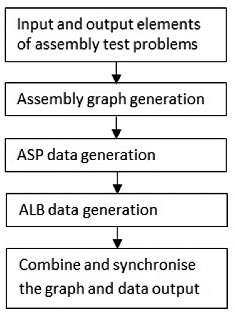
Test problem generator development flow.

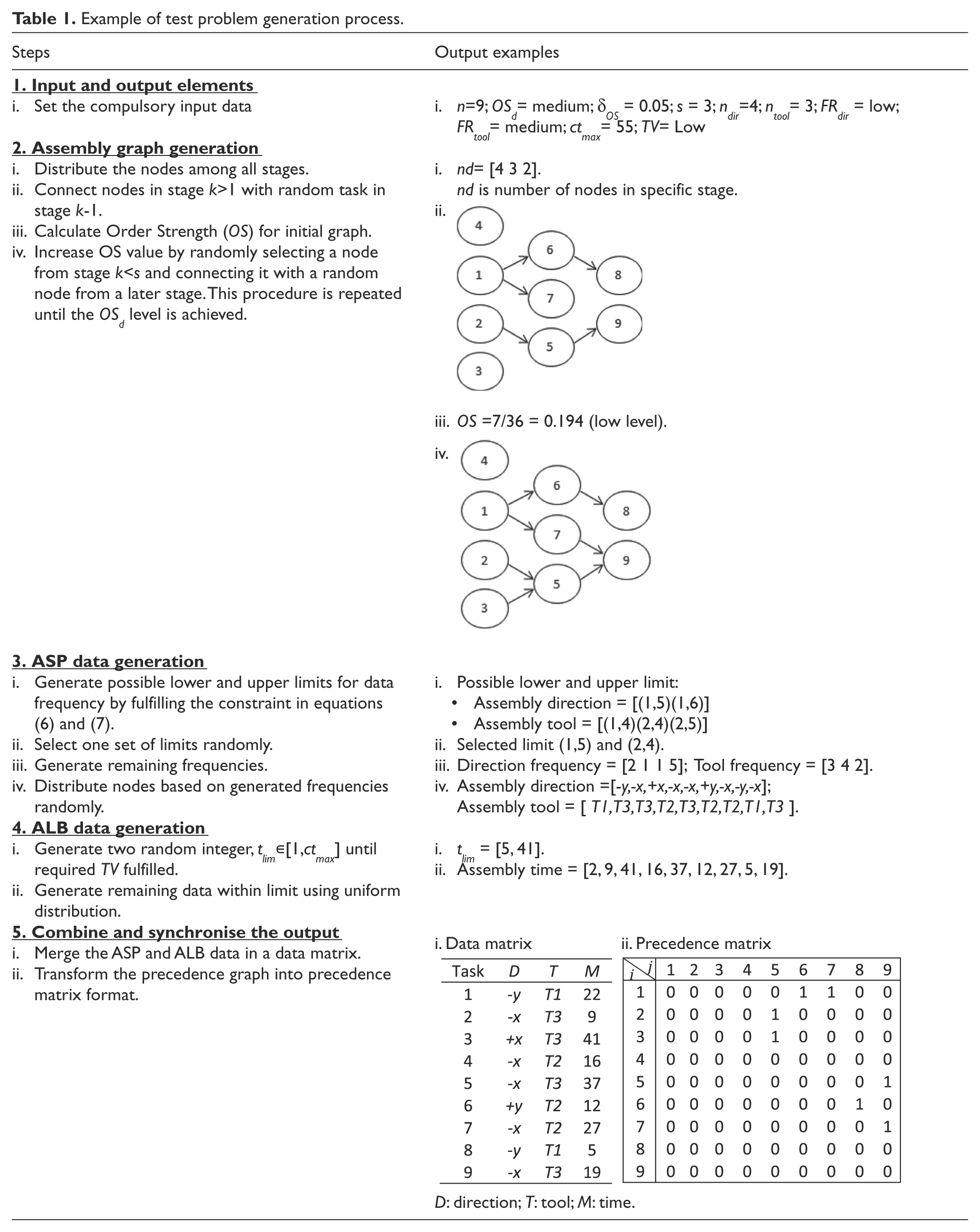
The first stage in developing the TPG is to identify the input and output elements. Next is the independent development of automated generators for assembly graph, ASP and ALB data. Finally, the outputs from graph and data generators are synchronised and combined to produce a complete test problem set. A worked example of the proposed TPG, with outputs for each step, is presented in Table 1.

Table 1.

Example of test problem generation process.

Steps	Output examples
1. Input and output elements
i. Set the compulsory input data	i. n=9; OS_d = medium; δ_OS = 0.05; s = 3; n_dir=4; n_tool = 3;FR_dir=low; FR_tool = medium; ct_max = 55; TV = Low
2. Assembly graph generation
i. Distribute the nodes among all stages.	i. nd = [4 3 2]. nd is number of nodes in specific stage.
ii. Connect nodes in stage k>1 with random task in stage k−1.	ii.
iii. Calculate Order Strength (OS) for initial graph.	iii. OS = 7/36 = 0.194 (low level).
iv. Increase OS value by randomly selecting a node from stage k<s and connecting it with a random node from a later stage. This procedure is repeated until the OS_d level is achieved.	iv.
3. ASP data generation
i. Generate possible lower and upper limits for data frequency by fulfilling the constraint in equations (6) and (7).	i. Possible lower and upper limit:
	• Assembly direction = [(1,5)(1,6)]
	• Assembly tool = [(1,4)(2,4)(2,5)]
ii. Select one set of limits randomly.	ii. Selected limit (1,5) and (2,4).
iii. Generate remaining frequencies.	iii. Direction frequency = [2 1 1 5]; Tool frequency = [3 4 2].
iv. Distribute nodes based on generated frequencies randomly.	iv. Assembly direction = [−y,−x,+x,−x,−x,+y,−x,−y,−x];Assembly tool = [T1,T3,T3,T2,T3,T2,T2,T1,T3].
4. ALB data generation
i. Generate two random integer, t_lim∈[1,ct_max] until required TV fulfilled.	i. t_lim = [5, 41].
ii. Generate remaining data within limit using uniform distribution.	ii. Assembly time = [2, 9, 41, 16, 37, 12, 27, 5, 19].
5. Combine and synchronise the output
i. Merge the ASP and ALB data in a data matrix.	i. Data matrix ii. Precedence matrix
ii. Transform the precedence graph into precedence matrix format.	D: direction; T: tool; M: time.

Input and output elements of assembly test problems

The mapping of input and output variables is shown in Figure 2. The tuneable inputs are presented in bold and italic font.

Figure 2.

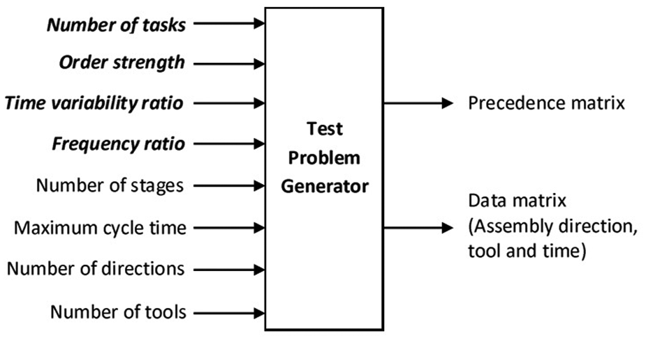
Problem generator input and output map.

Tuneable input elements

The tuneable input elements are variables that are used to control the problem difficulty generated by the TPG. In this work, one new tuning variable is proposed and the rest are adopted from previous works. The TPG is conceptually divided into two parts: the generation of assembly graphs and the generation of assembly data. The next section will discuss the tuneable input variables for each part. Although the tuneable input variables for ALB has been discussed in earlier works, no clear link has been suggested in literature between input and specific difficulty levels for ASP.¹³

Tuneable input for assembly graph

Two tuneable inputs will be used to generate precedence at a specific complexity level. The first input variable to measure graph complexity is n, the number of nodes in a graph. In ASP and ALB contexts, graph nodes represent assembly tasks for a given problem. The number of possible assembly sequences will exponentially increase with the number of nodes. In surveyed literature, the size of ASP problems varies between 5 to 75 nodes; in ALB, 86% of surveyed ALB articles used between 7 to 150 nodes, while the remaining 14% used up to 300 nodes.

Another graph input variable conceptually linked to graph difficulty is order strength. Order strength (OS) measures the relative number of precedence relation in a graph. By increasing the relative number of precedence relations, the resulting graph is expected to be more complicated.^13,15 Order strength is defined as a total number of ordering relation in transitive closure divided by the possible number of ordering relation for particular graph. The order strength is calculated as

OS = \frac{R}{P}

(1)

where R is the total number of ordering relations and P is the possible number of ordering relations

P = \frac{n (n - 1)}{2}

(2)

where n is the number of nodes.

The order strength value varies between [0, 1]. OS = 0 shows that there is no precedence relation in the graph and OS = 1 shows that there is only one feasible sequence for a particular problem. The order strength attribute is used together with order strength tolerance (δ_OS) since it is difficult (impossible in some cases) to meet the exact order strength value.

Tuneable input for assembly data

Previously, a number of time-related measures for ALB data have been proposed, such as ratio between maximum and minimum completion time between assembly lines,¹⁷ standard deviation,¹⁵ and time variability ratio. A time variability ratio (TV) has consistently been used in previous works and is selected for use in this work. A time variability ratio indicates the range of task time of all tasks dispersed between the assembly lines. A time variability ratio is calculated as

TV = \frac{t_{\max}}{t_{\min}}

(3)

t_{\max} \geq \frac{1}{3} c t_{\max}

(4)

where t_max is the maximum task time, t_min is the minimum task time and ct_max is the maximum cycle time.

A smaller time variability ratio value indicates that existing task times are distributed in a smaller range, which leads to an increased level of problem complexity. The t_max constraint in equation (4) is introduced to avoid generation of uniformly small task time, which leads to inconsistency of difficulty levels. The ct_max constraint is explained in ‘Other input elements’.

Meanwhile, in the ASP problem domain, no variable for measuring data complexity has been established. In this work, the ASP data considered are assembly directions and assembly tools. This type of data can be measured by considering how many times (i.e. frequency) a similar direction or tool appears in the problem. A common optimisation objective is to minimise direction or tool changes in a sequence of tasks. Thus, the frequency ratio (FR) is proposed to be used as an input variable that measures ASP data complexity.

FR = \frac{f_{\min}}{f_{\max}}

(5)

where f_min is the minimum data frequency and f_max is the maximum data frequency.

Data with a higher frequency ratio is harder to arrange to achieve the minimum number of changes because the choice and variability of data are high. This type of data will usually produce a higher number of changes compared with smaller frequency ratio data. The details of graph and assembly data attributes level are shown in Table 2. In this table, the attribute level for the ‘number of nodes’ is proposed based on a survey on problem sizes, as mentioned in ‘Tuneable input elements’, while the proposed classification of frequency ratio and time variability levels are based on a few initial tests. The proposed classification of order strength levels is adopted from literature review.¹⁶

Table 2.

Assembly graph and assembly data attribute levels.

Attributes	Low	Medium	High
Number of nodes, n	n≤20	20<n≤70	n>70
Order strength, OS	OS≤0.2	0.2<OS≤0.6	OS>0.6
Time variability ratio, TV	TV>6.5	2.5<TV≤6.5	TV≤2.5
Frequency ratio, FR	FR≤0.2	0.2<FR≤0.6	FR>0.6

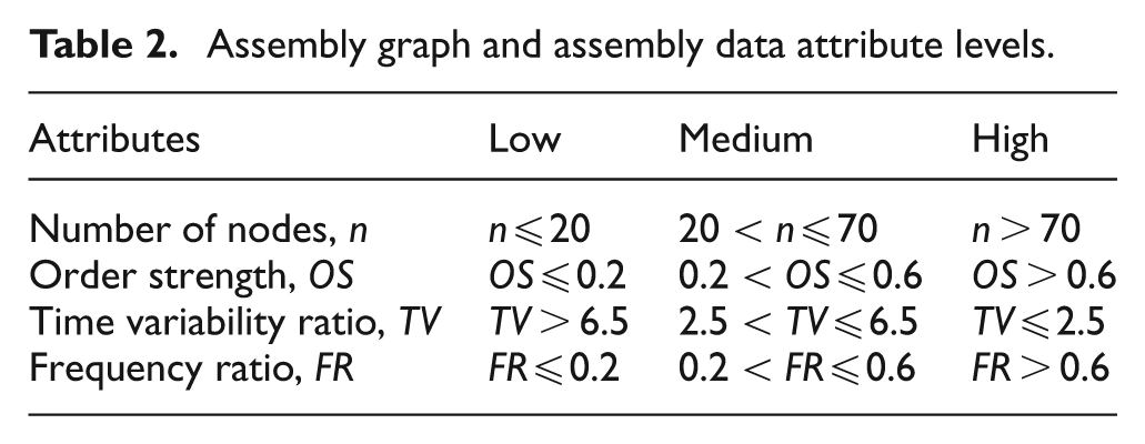
The tuneable input variables are classified into low, medium and high levels because of nonlinearity of the problem. Although the general trend of problem difficulty over tuneable variables can be predicted, when tuning for a targeted difficulty level, too small variable changes may lead to inconsistent difficulty levels. The classification of level difficulties, as in Table 2, can be used as a guideline for users in selecting appropriate difficulty levels for their use. To reduce the possibility of inconsistent difficulty levels, it is suggested to use the midpoint of the medium level to generate a medium difficulty problem.

Other input elements

Apart from the tuneable elements, there are other ‘compulsory’ inputs that are required for generating a complete problem. Although some of these variables have implications to the problem difficulty level, they are not used here as a means to control the problem difficulty because of a lack of agreement in literature. These inputs are: number of stages (s), maximum cycle time (ct_max), number of assembly direction (n_dir) and number of assembly tool (n_tool). Number of stages (s) refers to the number of columns that contain nodes in a specific precedence graph. In Figure 3, the example graph consists of three stages (hence s = 3), which are shown separated by dotted lines. This variable determines the basic shape of the graph, where a smaller number of stages will produce graphs with more parallel nodes. The maximum cycle time (ct_max) is the upper limit of allowable cycle time. This variable is calculated from the required production rate of the assembly line. The number of directions and number of tools are also required to generate ASP data.

Figure 3.

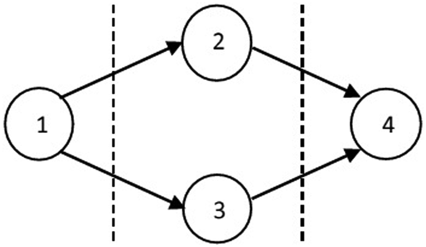
Example of precedence graph.

Another important element of the TPG is the pseudo-random number generator that underlies most of the data generation algorithm. In this work, the pseudo-random generator used is Mersenne Twister with the range between [0, 2³²−1] for a 32-bit integer.¹⁸ Appropriate use of seed values ensures that all results are reproducible.

Output elements

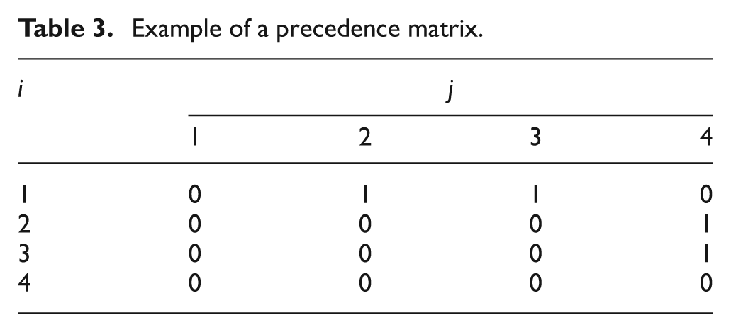
There are two sets of outputs generated by the proposed TPG. The first output is the assembly precedence graph (e.g. Figure 3), represented by a precedence matrix, which is an n × n matrix filled with 1 or 0 values (Table 3). The left-most column shows assembly tasks and the top row shows the follower tasks. The value 1 shows that the task j must be performed after task i.

Table 3.

Example of a precedence matrix.

i	j
	1	2	3	4
1	0	1	1	0
2	0	0	0	1
3	0	0	0	1
4	0	0	0	0

The second output is a data matrix that consists of assembly directions, assembly tools and assembly time associated with every task. This data is generated according to the required difficulty level as determined in tuneable input variables.

Assembly graph generation

In this work, the systematic graph generation method is adopted from Otto’s work.¹⁶ The five steps below are as proposed in that work.

Step 1. Provide all the compulsory inputs. The compulsory inputs are number of nodes (n), desired order strength (OS_d), order strength tolerance (δ_OS) and number of stages (s).

Step 2. Generate and distribute the nodes in all stages using uniform distribution.

Step 3. Connect every node in stage k >1 with exactly one random node in stage k − 1. This step is important to keep the nodes in their original stages.

Step 4. Calculate the order strength using equation (1). If the order strength is within OS_d ± δ_OS, then terminate the process. Otherwise, continue with Step 5.

Step 5. Select a node i in stage k < s and insert an arc to a random node j in stage m > k until the desired order strength is achieved. A direct arc from node i to node j is allowed only if:

Task i has no restriction, such as isolated node or special structure;

The order strength values have not exceeded the desired upper limit.

ASP data generation

In this work, the ASP data that are considered are ‘assembly direction’ and ‘assembly tool change’. The following steps are applied to generate these data. Besides number of tasks, n, the required input in ASP data generation is ASP ‘data frequency ratio’, FR.

Step 1. Calculate all possible lower (L_limit) and upper (U_limit) limits of data frequencies according to FR. The L_limit and U_limit represent the minimum and maximum number of times that a particular direction or tool appear in the generated problem. These limits must fulfil the following constraints

U_{limit} \times (n_{type} - 1) + L_{limit} \geq n

(6)

L_{limit} \times (n_{type} - 1) + U_{limit} \leq n

(7)

Equations (6) and (7) ensure that the summation of generated data within upper and lower limits matches the number of tasks, n. In these equations, n_type represent the number of direction (n_dir) or number of tool (n_tool) type. In this work, six major direction axes (+x, −x, +y, −y, +z, −z) are considered, thus n_type for n_dir is equal to six. Meanwhile the n_type for n_tool depends on the number of tool types in a particular assembly line.

Step 2. Randomly select a pair of lower and upper limits from the set of possible limits determined in Step 1. Generate remaining data frequencies using uniform distribution. The summation of data frequencies must be equal to n.

Step 3. Generate the ASP data based on frequencies (Step 2) in random order.

ALB data generation

The ALB data to be generated is the ‘task time’ for all nodes. The required inputs are ‘maximum cycle time’ (ct_max) and ‘time variability ratio’ (TV). This data is generated in two steps:

Step 1. Calculate all possible limit of task time based on TV. The upper limit must not exceed ct_max. Randomly select an upper and lower limit from all possible limit pairs.

Step 2. Generate the remaining task times between upper and lower limits using uniform distribution.

Combine and synchronise the graph and data output

Synchronisation of ASP-specific and ALB-specific outputs is straightforward because both ASP and ALB representations are both developed using the same assembly task basis.¹⁹ Data generated in ‘ASP data generation’ and ‘ALB data generation’ are directly linked with assembly tasks and no further adjustment is needed. In this synchronisation step, the output data consisting of ASP data from ‘ASP data generation’ and ALB data from ‘ALB data generation’ are combined to establish a data matrix. In the data matrix, the assembly direction data is located on the first column, assembly tool data in the second column and assembly data for ALB in the third column.

The final process in this step is to transform the precedence graph into a precedence matrix as explained in ‘Output elements’. This is an important process to synchronise the format of the assembly graph into readable computer language.

Experimental design

This section describes the set-up of the experimental design to assess problems generated using the proposed TPG. The experiment is divided into two phases. In Phase 1, the experiment will focus on the ability of the TPG to generate problems at a desired complexity level by manipulating the tuneable input attributes. Then, in Phase 2, the generated problems from the TPG will be used to evaluate the performance of a set of selected algorithms. The purpose of the second phase experiment is to identify if the generated problems from the TPG can be used to characterise the best and worst performance of each algorithm.

Phase 1. Testing of tuneable input

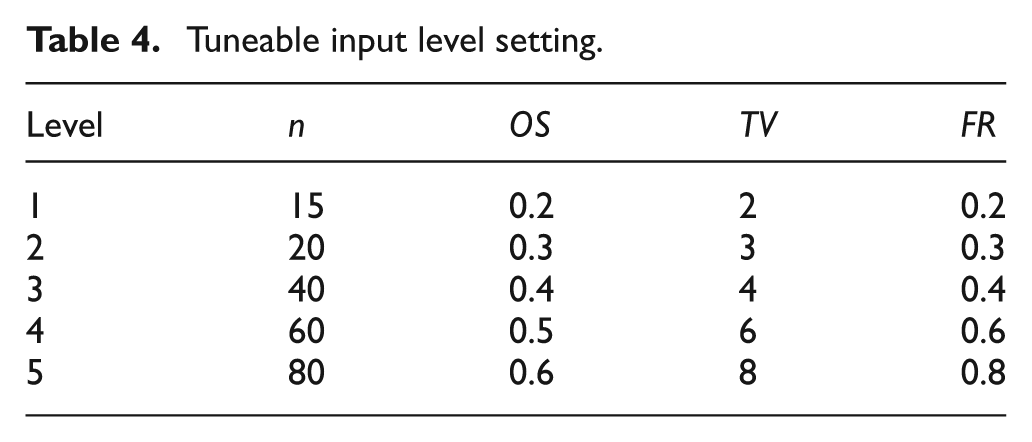
The experiment in this phase is conducted by dividing all the tuneable input variables into five levels, as presented in Table 4.

Table 4.

Tuneable input level setting.

Level	n	OS	TV	FR
1	15	0.2	2	0.2
2	20	0.3	3	0.3
3	40	0.4	4	0.4
4	60	0.5	6	0.6
5	80	0.6	8	0.8

A reference variable setting (datum) is selected as a baseline, while the rest of the problem variable settings are generated by changing only one variable value at a time. In this case, level 3 is selected as the reference variable setting because it is in the middle between the minimum and maximum value. The complete experimental table for Phase 1 is shown in Table 5.

Table 5.

Experimental table for Phase 1.

Problem	n	OS	TV	FR
1	40	0.4	4	0.4
2	15	0.4	4	0.4
3	20	0.4	4	0.4
4	60	0.4	4	0.4
5	80	0.4	4	0.4
6	40	0.2	4	0.4
7	40	0.3	4	0.4
8	40	0.5	4	0.4
9	40	0.6	4	0.4
10	40	0.4	2	0.4
11	40	0.4	3	0.4
12	40	0.4	6	0.4
13	40	0.4	8	0.4
14	40	0.4	4	0.2
15	40	0.4	4	0.3
16	40	0.4	4	0.6
17	40	0.4	4	0.8

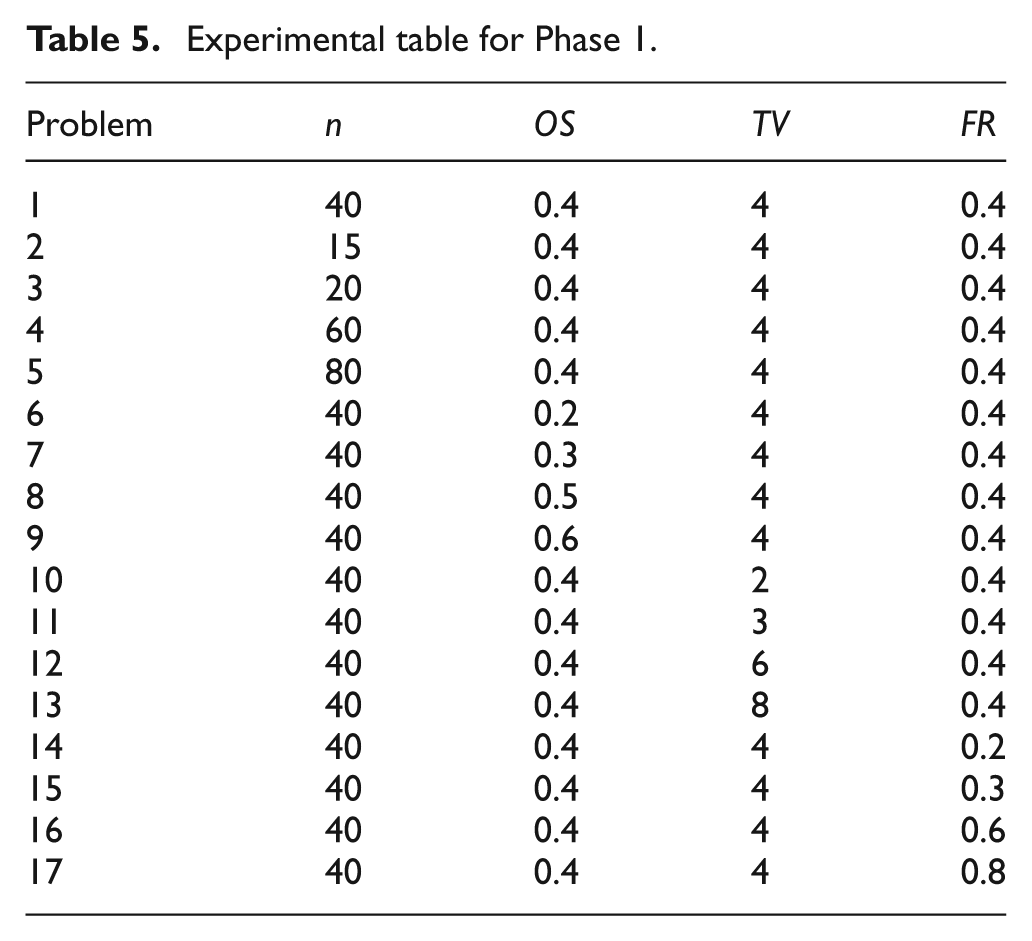
From Table 5, 17 test problems are generated by changing one variable at a time. Problem 1 represents the reference variable setting, problems 2–5 examine the effect of n, problems 6–9 for effect of OS, problems 10–13 for effect of TV and problems 14–17 for effect of FR.

In order to solve precedence graphs, the topological sort algorithm is used to generate feasible assembly sequences. This approach will ensure that the generated sequences are always feasible by sorting the nodes into ‘available’ and ‘unavailable’ tasks, during the sequence generation process.²⁰

To test the generated problems, three different algorithms were selected for each problem type. For an ASP problem, a multi-objective genetic algorithm (MOGA) that was used in Choi et al.²¹ is chosen. This algorithm is selected because, in common with this work, it used task-based representation in representing ASP problems. Additionally, a genetic algorithm is one of the most frequently used algorithms for solving and optimising ASP problems.² In this algorithm, the fitness function for ASP is

f_{1} = \frac{dc}{d c_{\max}} + \frac{tc}{t c_{\max}}

(8)

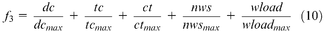
where dc is the number of direction changes, tc is the number of tool changes, dc_max is the maximum possible number of direction changes, tc_max maximum possible number of tool changes and dc_max, tc_max is the number of nodes – 1.

To test the ALB problem, an ant colony optimisation (ACO) algorithm that has been used for a simple assembly line balancing problem (SALBP) in Bautista and Pereira²² is used. This algorithm is selected based on citation popularity. In addition, an ant colony algorithm is also one of the frequently used algorithms to solve and optimise the ALB problem.² In this algorithm, the fitness function is designed as

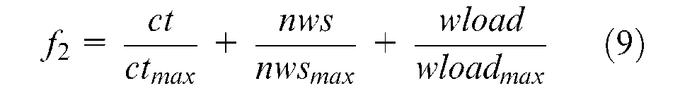
f_{2} = \frac{ct}{c t_{\max}} + \frac{nws}{nw s_{\max}} + \frac{wload}{wloa d_{\max}}

(9)

where ct is the cycle time, nws is the number of workstations, wload is the workload variance, ct_max is the maximum possible cycle time, nws_max is the maximum possible number of workstations and wload_max is the maximum possible workload variance.

Finally, for an integrated ASP and ALB problem, a hybrid genetic algorithm (HGA) that used in Chen et al.³ is selected. This algorithm is also selected based on the popularity of this work for integrated ASP and ALB. The fitness function for this problem is designed as

f_{3} = f_{1} + f_{2}

f_{3} = \frac{dc}{d c_{\max}} + \frac{tc}{t c_{\max}} + \frac{ct}{c t_{\max}} + \frac{nws}{nw s_{\max}} + \frac{wload}{wloa d_{\max}}

(10)

Phase 2. Algorithm testing using generated problems

In Phase 2, the algorithms’ performance to generate a Pareto optimal solution for a combined ASP and ALB problem are tested. The purpose of this test is to determine whether the problems generated by the TPG have sufficient variety that enables users to perceive differences in algorithm performance. To perform this test, the MOGA and ACO algorithm, previously used to optimise ASP and ALB independently, will be used to optimise a combined ASP and ALB problem alongside a HGA. The objective function set for this experiment is as follows.

f₁ = minimise number of direction change

f₂ = minimise number of tool change

f₃ = minimise cycle time

f₄ = minimise number of workstations

f₅ = minimise workload deviation

In order to evaluate the performance of each algorithm when dealing with different complexity problems, the following performance indicators are adopted from Deb²³ and Yoosefelahi et al.²⁴ are used.

Number of non-dominated solutions in Pareto optimal, : Show the number of non-dominated solutions generated by each algorithm in Pareto solution. Higher indicates better algorithm performance.

Error ratio, ER: ER is given by dividing the number of solutions which are not members of the Pareto optimal set with the total number of solutions generated by algorithm q. Smaller ER indicates better algorithm performance.

Generational distance, GD: GD finds an average distance of solution with the nearest Pareto optimal solution. A smaller GD indicates better algorithm performance.

G D_{q} = \frac{\sum_{i = 1}^{s_{q}} d_{i}}{s_{q}}

(11)

where s_q is the number of solutions generated by algorithm q

d_{i} = \min_{k = 1}^{P} \sqrt{\sum_{m = 1}^{M} {(f_{m}^{(i)} - f_{m}^{* (k)})}^{2}}

(12)

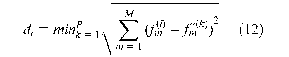
where $f_{*}^{(i)}$ is the mth objective function value of solution i and $f_{m}^{* (k)}$ is the mth objective function value of the kth member of the Pareto optimal set.

iv. Spacing: This indicator measures the relative distance between each solution.

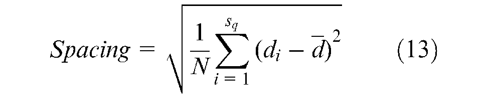
Spacing = \sqrt{\frac{1}{N} \sum_{i = 1}^{s_{q}} {(d_{i} - \bar{d})}^{2}}

(13)

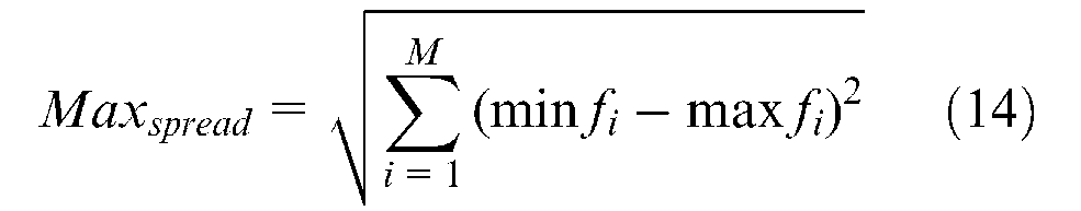
where $d_{i}$ is distance between solution i and the nearest solution, while $\bar{d}$ is the average of all $d_{i}$ . Smaller Spacing indicates better uniformity of space between solutions.

v. Maximum Spread, Max_spread: Measures the extent of solution distribution found by the algorithm. Larger maximum spread is better.

Ma x_{spread} = \sqrt{\sum_{i = 1}^{M} {(min f_{i} - max f_{i})}^{2}}

(14)

Results and discussion

Phase 1: Results

The output from Phase 1 experiments are presented in Figures 4 to 7, showing the average of best fitness value from ten runs.

Figure 4.

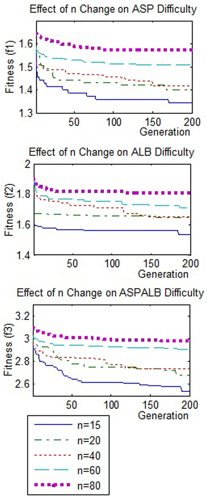
Average of best fitness for a range of n (number of tasks).

Figure 5.

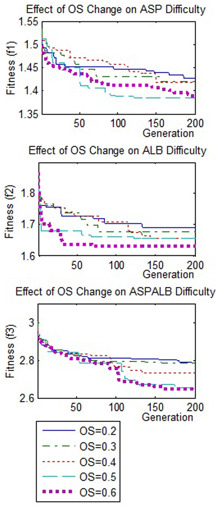
Average of best fitness for different OS value.

Figure 6.

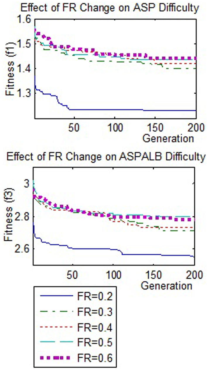
Average of best fitness for different frequency ratio.

Figure 7.

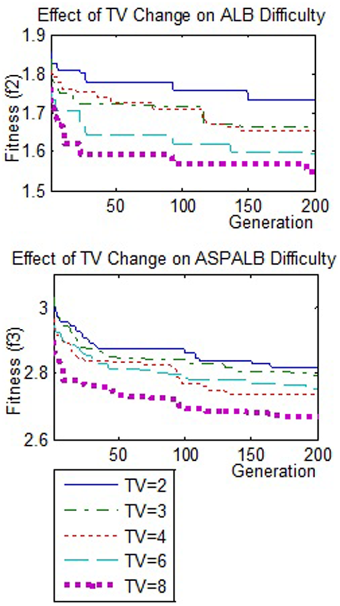
Average of best fitness for different time variability ratio.

Number of tasks (n)

Figure 4 shows the effect of n on the ASP, ALB and combined ASPALB problem difficulties. In all cases, the problems with a larger number of tasks tend to be found to have better fitness, although they have similar tuneable input setting for OS, FR and TV. This output pattern is related with increments of problem difficulties when the number of tasks is increased. The output trend is also consistent with previous works, such as in Scholl,¹³ Bhatterji and Sahu¹⁵ and Otto et al.¹⁶

Order strength (OS)

Figure 5 shows the effect of OS change for ASP problems with 15, 20, 40, 60 and 80 tasks. In these graphs, the ASP problems with high OS values tend to produce better fitness values compared with low and medium OS values. A similar output pattern is also found in ALB and combined ASPALB problems, as shown in Figure 5. This result indicates that problems with higher OS values will have lesser difficulty levels compared with low OS values. This finding corroborates a few previous works,^25–27 while contradicting a few works that associate higher OS values with greater complexity.^13,16

This mismatch is due to the dissimilar approaches used in solving the precedence graph. In the works that directly used generated permutation as an assembly sequence, precedence graphs with higher OS values are harder to solve. Direct permutation has a high probability of generating infeasible sequences; since the numbers of precedence constraints in high OS graphs are higher than low OS graph while the search space for both conditions remains the same.

On the other hand, in the works that ensures the feasibility of sequence, such as using topological sort, the precedence graph with higher OS is easier to solve, because of differences in the search space size. The OS value directly influences the number of possible feasible sequences in a precedence graph. In this case, the number of feasible sequences in high OS is smaller than in low OS, because the precedence constraints limit the flexibility of re-sequencing. Since the search space for the precedence graph with high OS is smaller than a low OS, it is easier to generate a solution with better fitness in high OS graphs than with low OS graphs.

Nevertheless, there is inconsistency in outputs for ASP with OS 0.5 and 0.6, ALB with OS 0.4 and 0.5 and combined ASPALB with OS 0.5 and 0.6. For these cases, the problem with a smaller OS emerges with better fitness compared with a larger OS. A likely explanation is that the chosen OS gaps for these problems are too small, since it does not happen in larger OS gaps, such as between OS 0.6 and 0.4 or smaller. Small OS gap means that there is only small search space difference between the two problems that has influenced the inconsistency of results for both conditions. Therefore, to ensure a clear separation between one difficulty levels with another, OS gaps that are too small should be avoided. More investigation is needed to fully investigate the effect of OS.

Frequency ratio (FR)

The output from the ASP problem in Figure 6 shows that the proposed complexity attributes of FR can be used to control the ASP data complexity.

ASP data with a high FR will have a wider range of choices that directly increase the size of search space. In contrast, ASP data with a low FR have a smaller search space owing to a more limited data variety. As a consequence, the algorithms found it more difficult to achieve minimum direction and tool change for ASP data with a higher FR.

Time variability ratio (TV)

ALB results in Figure 7 confirm that the time variability ratio adopted from previous works is effective to control the assembly time data complexity.^13,16

The assembly times with higher TV are easier to arrange because the combination of small and large task times tend to fit the cycle time better than uniformly large task times (low TV). Finally the combined ASPALB outputs in this figure clearly show that the TV input variable is able to control the assembly data difficulties as expected.

The results of the tuneable input test show that the ASP and ALB problem complexity can be controlled via the input attributes of the TPG. Although the early assumption that the precedence graph with higher OS will have greater complexity is unfounded, this attribute’s usefulness is maintained by redefining its value: to generate precedence graphs with a low complexity, a higher OS level must be used, while for graphs with a high complexity, the OS must be set to the lower level. It is found that the selection of a tuneable input level is also important to ensure that the desired problem difficulty is achieved. Selection of proper gaps between one level to another is very important to avoid inconsistent problem difficulty.

In order to test the significance of the results, statistical tests are performed. In this case, an ANOVA test is carried out to test if there are any significant differences between the results of one level with results from another level. The null hypothesis stated that there would be no difference among five tuneable input levels means. The summary of the ANOVA test is presented in Table 6.

Table 6.

Summary of the ANOVA test.

	n change	OS change	FR change	TV change
SSB	16.4897	0.9418	7.3437	2.5119
SSW	3.2268	3.7542	2.181	2.1205
SST	19.7165	4.6961	9.5247	4.6324
MSB	4.1224	0.2354	1.8359	0.6280
MSW	0.0032	0.0037	0.0021	0.0021
f	1288.25	63.62	874.23	299.05

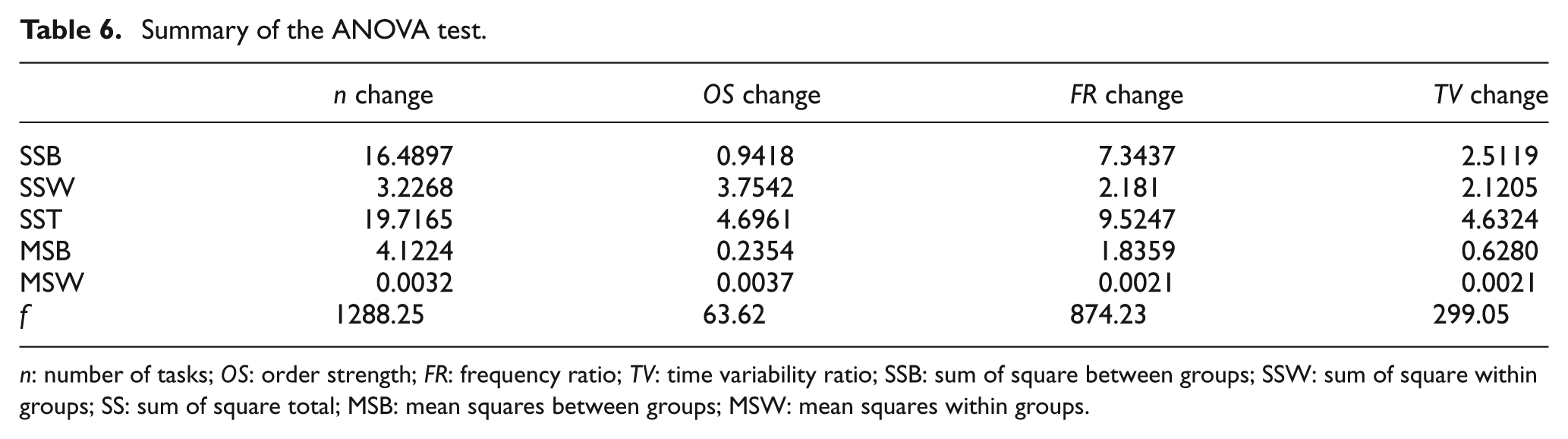
n: number of tasks; OS: order strength; FR: frequency ratio; TV: time variability ratio; SSB: sum of square between groups; SSW: sum of square within groups; SS: sum of square total; MSB: mean squares between groups; MSW: mean squares within groups.

In this case, the critical f-value (f*) that is acquired with a 0.05 level of significance from the f-distribution table is 2.22.²⁸Table 6 consistently shows larger f-values compared with f*. Since all the f-values are larger than f*, the null hypothesis for all tuneable input is rejected. In other words, it shows that at 0.05 confidence levels, there are statistically significant differences between levels for n, OS, FR and TV. However, this test does not tell us the exact groups or levels that have statistically significant difference in means. Therefore, a posteriori test known as Tukey’s honestly significant different test (Tukey’s HSD test) is performed.

Tukey’s HSD test compares the mean of the rejected null hypothesis with the means of other groups to identify if there is any significant difference between the mean of one level with another. The value of the absolute difference between two means will be compared with a critical HSD as proposed in the Tukey’s table.²⁸ The summary of the Tukey’s HSD test at 0.05 confidence interval is presented in Table 7. From Table 7, the absolute mean difference between two levels for n and TV consistently indicates larger values than the critical HSD value. It shows that there are significant differences in all levels for n and TV. It means that the problem difficulties for these variables can be statistically distinguished between each level.

Table 7.

Summary of Tukey’s HSD test.

Variable (critical HSD)	Comparison level		Absolute mean difference
n (0.015536)	15	20	0.1331
	15	40	0.1497
	15	60	0.2929
	15	80	0.3658
	20	40	0.0166
	20	60	0.1598
	20	80	0.2327
	40	60	0.1432
	40	80	0.2161
	60	80	0.0729
OS (0.016759)	0.2	0.3	0.008
	0.2	0.4	0.0292
	0.2	0.5	0.068
	0.2	0.6	0.0755
	0.3	0.4	0.0212
	0.3	0.5	0.06
	0.3	0.6	0.0675
	0.4	0.5	0.0388
	0.4	0.6	0.0169
	0.5	0.6	0.0075
FR (0.012773)	0.2	0.3	0.192
	0.2	0.4	0.1954
	0.2	0.5	0.2301
	0.2	0.6	0.2256
	0.3	0.4	0.0034
	0.3	0.5	0.0381
	0.3	0.6	0.0336
	0.4	0.5	0.0347
	0.4	0.6	0.0302
	0.5	0.6	0.0045
TV (0.009053)	2	3	0.0205
	2	4	0.0708
	2	6	0.0894
	2	8	0.1453
	3	4	0.0503
	3	6	0.0389
	3	8	0.1248
	4	6	0.0114
	4	8	0.0745
	6	8	0.0859

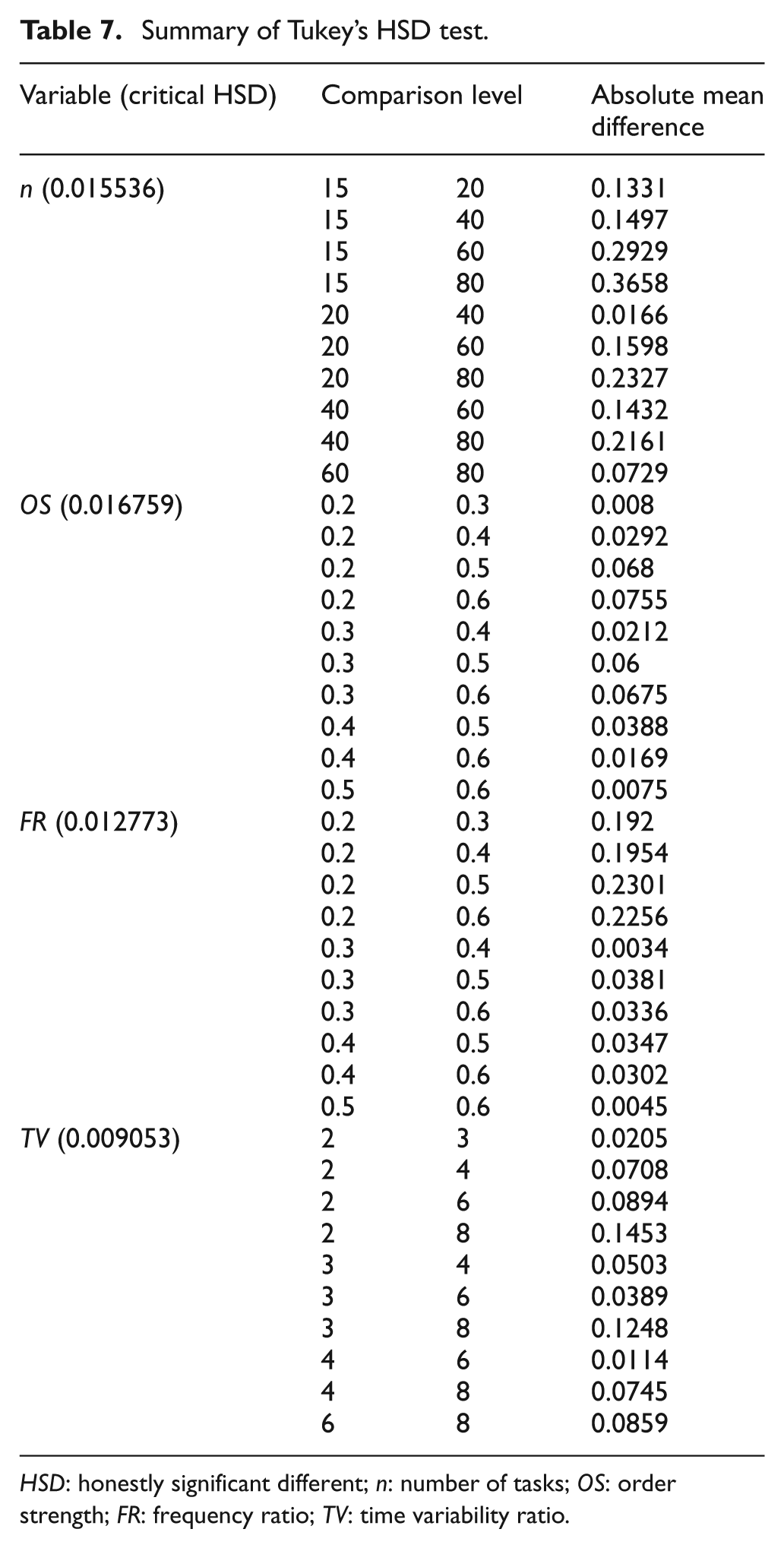
HSD: honestly significant different; n: number of tasks; OS: order strength; FR: frequency ratio; TV: time variability ratio.

Meanwhile, in the OS and FR variables, the absolute mean difference also shows larger values than critical HSD except for the cases between OS values of 0.2 and 0.3, OS values 0.5 and 0.6, FR values 0.3 and 0.4, and FR values 0.5 and 0.6. This result is related to the selection of appropriate gaps between levels, since it only occurs between adjacent levels. Consistent with earlier discussions on the effect of OS change on the problem difficulties (Figure 5), too small gaps between consecutive levels should be avoided.

Phase 2: Results

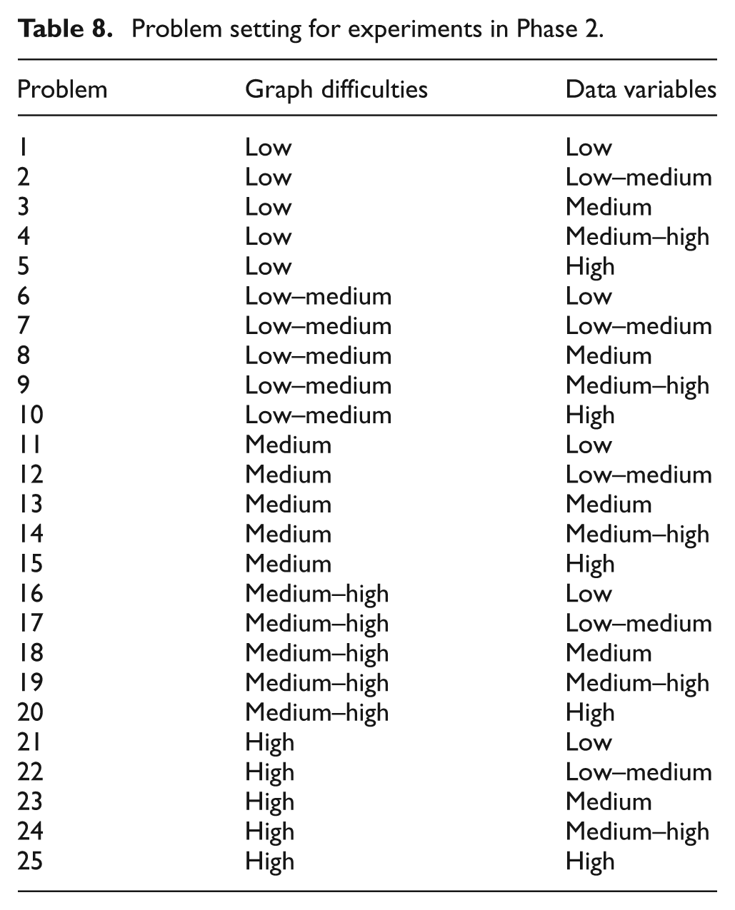
In this phase, 25 problems with different difficulty settings are used to demonstrate the usefulness of the TPG for testing the performance of algorithms. The set-up is for multi-objective optimisation of ASP, ALB, and ASPALB problems. The assembly problem for this experiment is set up as in Tables 8 and 9.

Table 8.

Problem setting for experiments in Phase 2.

Problem	Graph difficulties	Data variables
1	Low	Low
2	Low	Low–medium
3	Low	Medium
4	Low	Medium–high
5	Low	High
6	Low–medium	Low
7	Low–medium	Low–medium
8	Low–medium	Medium
9	Low–medium	Medium–high
10	Low–medium	High
11	Medium	Low
12	Medium	Low–medium
13	Medium	Medium
14	Medium	Medium–high
15	Medium	High
16	Medium–high	Low
17	Medium–high	Low–medium
18	Medium–high	Medium
19	Medium–high	Medium–high
20	Medium–high	High
21	High	Low
22	High	Low–medium
23	High	Medium
24	High	Medium–high
25	High	High

Table 9.

Attribute settings for different graph and data difficulty levels.

Level	Graph difficulty		Data difficulty
	n	OS	FR	TV
Low	15	0.6	0.2	8
Low–medium	20	0.5	0.3	6
Medium	40	0.4	0.4	4
Medium–high	60	0.3	0.5	3
High	80	0.2	0.6	2

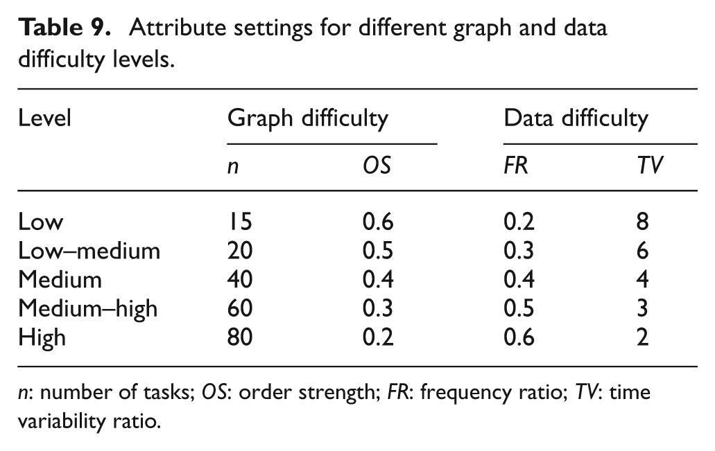
n: number of tasks; OS: order strength; FR: frequency ratio; TV: time variability ratio.

The tuneable input for these test problems are grouped into graph difficulty (n and OS variables) and data difficulty (FR and TV variables). The data of test problems that are used in this work can be downloaded from http://public.cranfield.ac.uk/s135489/ASP_ALB_Test_Problems_Data.zip.

The results from Phase 2 experiments are summarised in Table 10. Numbers in brackets are weighting values that are assigned to each algorithm based on its performance for the respective indicator. For every indicator in a given problem, the best result is assigned a weight value of 3, while the second and third positions are assigned weight values of 2 and 1, respectively. Then, the algorithm ranking is made through comparison of the weighted sums.

Table 10.

Summary of the result of experiments on selected multi-objective algorithms.

Problem	Algorithm	$\tilde{η}$	ER	GD	Spacing	Max _spread	Sum of weight	Rank
1	MOGA	15(2)	0.5946(2)	1.0340(1)	1.2913(2)	34.2251(2)	9	2
	ACO	12(1)	0.6250(1)	0.9694(2)	1.1781(3)	34.1030(1)	8	3
	HGA	24(3)	0.2727(3)	0.3565(3)	2.2112(1)	36.9763(3)	13	1
2	MOGA	22(2)	0.4359(2)	0.7180(2)	1.0435(2)	34.2097(3)	11	2
	ACO	11(1)	0.6452(1)	1.1590(1)	1.4938(1)	33.3108(2)	6	3
	HGA	35(3)	0.1667(3)	0.2681(3)	0.8956(3)	31.2778(1)	13	1
3	MOGA	12(2)	0.7447(1)	1.1370(2)	1.0293(3)	40.2682(2)	10	2
	ACO	10(1)	0.6429(2)	1.1764(1)	1.8612(1)	38.1782(1)	6	3
	HGA	40(3)	0.1489(3)	0.2517(3)	1.4235(2)	41.1657(3)	14	1
4	MOGA	29(2)	0.3556(1)	0.4950(2)	1.3678(2)	36.5902(1)	8	3
	ACO	26(1)	0.2973(3)	0.4366(3)	1.7489(1)	38.3385(2)	10	2
	HGA	35(3)	0.3519(2)	0.5074(1)	1.1018(3)	38.5984(3)	12	1
5	MOGA	11(2)	0.5926(2)	0.9460(2)	1.2987(3)	33.5636(2)	11	2
	ACO	10(1)	0.6429(1)	1.0924(1)	1.3385(2)	34.3586(3)	8	3
	HGA	22(3)	0.2667(3)	0.3276(3)	1.6657(1)	34.3586(3)	13	1
6	MOGA	13(1)	0.7869(1)	1.7381(1)	1.6819(1)	39.5870(1)	5	3
	ACO	25(3)	0.5098(2)	1.3454(2)	1.6183(2)	39.6918(2)	10	2
	HGA	40(2)	0.4030(3)	0.6576(3)	1.4541(3)	40.0436(3)	15	1
7	MOGA	16(2)	0.6098(1)	1.1300(1)	1.6974(1)	37.2650(1)	6	3
	ACO	16(2)	0.5789(2)	1.0099(2)	1.5133(2)	39.3564(3)	11	2
	HGA	41(3)	0.3051(3)	0.5166(3)	1.1344(3)	39.0404(2)	14	1
8	MOGA	17(2)	0.7018(1)	1.1665(1)	1.3567(2)	39.0331(3)	9	2
	ACO	16(1)	0.5429(2)	1.0410(2)	1.8336(1)	37.3966(1)	7	3
	HGA	40(3)	0.3443(3)	0.5396(3)	0.9635(3)	37.7713(2)	14	1
9	MOGA	17(2)	0.6909(1)	1.1311(1)	1.1018(3)	39.7311(2)	9	2
	ACO	14(1)	0.5882(2)	1.0600(2)	1.6150(2)	38.1256(1)	8	3
	HGA	36(3)	0.4930(3)	0.8795(3)	1.7604(1)	44.9119(3)	13	1
10	MOGA	16(1)	0.6667(1)	1.2655(1)	1.5753(1)	36.4029(1)	5	3
	ACO	25(2)	0.5763(2)	1.1164(2)	1.3033(2)	37.8426(3)	11	2
	HGA	30(3)	0.5238(3)	0.7406(3)	1.0246(3)	37.6970(2)	14	1
11	MOGA	17(1)	0.8496(1)	1.9129(1)	1.3149(3)	45.1158(1)	7	3
	ACO	60(2)	0.5000(2)	0.9915(2)	1.3560(2)	46.4900(3)	11	2
	HGA	86(3)	0.3723(3)	0.7732(3)	1.4197(1)	45.4979(2)	12	1
12	MOGA	24(1)	0.7073(1)	1.7056(1)	1.8150(1)	48.4041(3)	7	3
	ACO	56(3)	0.3253(3)	0.6771(3)	1.4082(3)	46.8911(1)	13	1
	HGA	44(2)	0.6271(2)	1.3069(2)	1.4886(2)	47.8308(2)	10	2
13	MOGA	20(1)	0.7701(1)	1.6837(1)	1.6846(2)	48.4191(2)	7	3
	ACO	42(2)	0.3731(2)	0.7612(3)	1.8370(1)	47.0473(1)	10	2
	HGA	74(3)	0.4351(3)	0.8760(2)	1.3466(3)	49.9341(3)	13	1
14	MOGA	56(2)	0.3778(3)	0.8536(2)	1.7669(1)	53.7493(1)	9	2
	ACO	65(3)	0.4348(2)	0.8321(3)	1.3163(2)	54.6819(3)	13	1
	HGA	49(1)	0.6797(1)	1.4087(1)	1.1580(3)	53.8050(2)	8	3
15	MOGA	15(1)	0.7857(1)	2.0094(1)	1.5541(3)	50.1276(3)	9	2
	ACO	31(2)	0.5441(2)	1.1165(2)	2.2496(1)	49.3039(1)	8	3
	HGA	49(3)	0.3194(3)	0.7035(3)	1.6625(2)	49.6062(2)	13	1
16	MOGA	38(1)	0.6696(1)	1.6155(1)	1.5986(2)	55.3575(3)	8	3
	ACO	86(3)	0.3723(3)	0.7880(3)	1.7949(1)	55.2207(2)	12	1
	HGA	69(2)	0.6124(2)	1.4092(2)	1.2798(3)	54.1806(1)	10	2
17	MOGA	30(1)	0.7391(1)	1.9710(1)	1.4983(3)	55.7943(3)	9	2
	ACO	62(2)	0.5000(3)	1.2519(2)	1.6083(1)	55.1087(1)	9	2
	HGA	73(3)	0.5494(2)	1.2063(3)	1.5393(2)	55.7024(2)	12	1
18	MOGA	22(1)	0.8182(1)	1.9982(1)	1.6087(2)	57.2777(1)	6	3
	ACO	88(3)	0.2000(3)	0.5709(3)	2.0579(1)	59.0822(3)	13	1
	HGA	74(2)	0.5747(2)	1.4657(2)	1.4820(3)	57.3599(2)	11	2
19	MOGA	42(1)	0.5922(1)	1.6303(1)	1.6454(3)	57.3484(2)	8	3
	ACO	49(2)	0.5664(2)	1.4639(2)	1.6960(2)	57.1157(1)	9	2
	HGA	74(3)	0.4559(3)	1.0453(3)	1.8645(1)	58.5914(3)	13	1
20	MOGA	33(1)	0.6972(1)	1.5315(1)	1.6453(2)	61.8964(2)	7	3
	ACO	66(2)	0.4000(3)	0.9788(2)	1.9603(1)	61.3480(1)	9	2
	HGA	84(3)	0.4650(2)	0.8983(3)	1.4834(3)	63.2256(3)	14	1
21	MOGA	17(1)	0.8411(1)	2.2525(1)	1.4918(2)	56.7749(1)	6	3
	ACO	117(3)	0.1761(3)	0.3228(3)	1.5736(1)	58.4656(3)	13	1
	HGA	57(2)	0.6780(2)	1.7245(2)	1.4484(3)	58.2365(2)	11	2
22	MOGA	44(1)	0.6944(1)	1.6900(1)	1.8500(2)	62.3752(2)	7	3
	ACO	90(3)	0.2857(3)	0.8241(3)	1.9158(1)	65.5746(3)	13	1
	HGA	70(2)	0.6410(2)	1.5881(2)	1.3136(3)	62.1336(1)	10	2
23	MOGA	21(1)	0.8397(1)	2.4638(1)	1.8718(2)	63.7124(2)	7	3
	ACO	46(2)	0.4458(3)	1.1937(3)	1.9034(1)	64.4027(3)	12	1
	HGA	74(3)	0.5912(2)	1.9811(2)	1.6302(3)	63.6888(1)	11	2
24	MOGA	39(1)	0.6286(2)	1.6486(1)	1.8588(2)	64.5943(1)	7	3
	ACO	71(3)	0.3238(3)	0.8033(3)	3.2717(1)	67.5944(3)	13	1
	HGA	61(2)	0.6494(1)	1.6160(2)	1.5992(3)	65.5225(2)	10	2
25	MOGA	57(1)	0.7077(2)	2.1692(2)	1.7039(2)	72.1097(1)	8	3
	ACO	105(3)	0.2606(3)	0.5954(3)	2.3302(1)	73.1415(3)	13	1
	HGA	74(2)	0.7218(1)	2.3913(1)	1.6459(3)	72.5640(2)	9	2

Numbers in brackets are weighting values from the best (weight = 3) to worst (weight = 1) performance.

$\tilde{η}$ : Number of nondominated solution in Pareto optimal; ER: error ratio; GD: generational distance; MOGA: multi-objective genetic algorithm; ACO: ant colony optimisation; HGA: hybrid genetic algorithm.

Based on the results in Table 10, the HGA consistently shows the best performance in all problems having low and low–medium graph difficulties (problems 1–10). Meanwhile, the MOGA shows better performance compare with the ACO algorithm for problems 1–3, but then showed inconsistent performance for problems 4–10. In problems 4–10, the ACO algorithm starts to overcome the MOGA performance in some cases.

Meanwhile, for the problems with medium and medium–high graph difficulties (problems 11–20), the HGA and ACO algorithms alternately lead the algorithms in the first rank. However, when the graph difficulty is increased to a high difficulty (problems 21–25), ACO has consistently shown a better performance and followed by HGA and MOGA. The relative performance of each algorithm is presented graphically in Figure 8.

Figure 8.

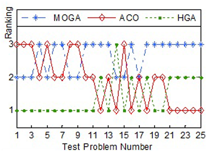
Algorithm’s ranking for the range of test problems.

Conclusions

In this work, a TPG with tuneable complexity for ASP and ALB problems has been proposed. A set of experiments has been conducted to assess the TPG. Experimental results confirm that problem complexities can be controlled by tuneable input variables.

The results from the Phase 1 experiments that test the effects of tuneable inputs confirm the ability of the TPG to generate problems with varying complexity levels. The problem difficulties will increase when using a larger number of tasks (n), smaller order strength (OS) value, larger frequency ratio (FR) or smaller time variability ratio (TV). As presented in the results, n and OS influence the assembly graph difficulties, while FR and TV influence the assembly data difficulties. The results of statistical tests confirmed that there are significant differences of the problem difficulties when changing the value of n and TV variables. On the other hand, the significant difference of problem difficulties can also be achieved by selecting the appropriate value for OS and FR, as suggested in Table 2.

The results of the algorithm performance experiment in Phase 2 show that the HGA consistently performed well in optimising problems with low and medium difficulties. Meanwhile, the ACO showed good performance in problems with a high level of difficulty. Based on the performance of both algorithms, the HGA is recommended for integrated ASP and ALB problems with low and medium difficulties, while the ACO is for ASP and ALB problems at high difficulty. These findings confirm that the problems generated by the TPG offer a sufficient range of problem varieties to be used in algorithm testing. The generated problems were found to be useful to identify the strengths and weaknesses of the tested algorithms.

Although further experiments are needed to confirm these strengths and weaknesses, the TPG has provided an important path by supplying a variety of ASP and ALB problems for systematic testing. Therefore, it can be concluded that the proposed TPG is able to generate combined ASP and ALB problems in a wide range of difficulties.

Footnotes

Funding

This research received no specific grant from any funding agency in the public, commercial, or not-for-profit sectors.

References

Wong

Fuh

JYH

. An enhanced assembly planning approach using a multi-objective genetic algorithm. Proc IMechE, Part B: J Engineering Manufacture 2006; 220(2): 255–272.

Rashid

MFF

Hutabarat

Tiwari

. A review on assembly sequence planning and assembly line balancing optimisation using soft computing approaches. Int J Advd Mfg Technol 2012; 59(1–4): 335–349.

Chen

. A hybrid genetic algorithm approach on multi-objective of assembly planning problem. Engng Applic Artif Intell 2002; 15(5): 447–457.

Tseng

Tang

. A sequential consideration for assembly sequence planning and assembly line balancing using the connector concept. Int J Prod Res 2006; 44(1): 97–116.

Marian

Luong

LHS

Abhary

. A genetic algorithm for the optimisation of assembly sequences. Computers Ind Engng 2006; 50(4): 503–527.

Chica

Cordón

Damas

. Multiobjective constructive heuristics for the 1/3 variant of the time and space assembly line balancing problem: ACO and random greedy search. Inf Sci 2010; 180(18): 3465–3487.

SmithSS. Using multiple genetic operators to reduce premature convergence in genetic assembly planning. Computers in Ind 2004: 54(1): 35–49.

Kilincci

Bayhan

. A Petri net approach for simple assembly line balancing problems. Int J Advd Mfg Technol 2006; 30(11–12): 1165–1173.

De Fazio

Whitney

. Simplified generation of all mechanical assembly sequences. IEEE J Robotics Autom 1987; RA-3(6): 640–658.

10.

Chen

Liu

. An adaptive genetic assembly-sequence planner. Int J Computer Integrated Mfg 2001; 14(5): 489–500.

11.

Smith

Liu

. The application of multi-level genetic algorithms in assembly planning. J Ind Technol 2001; 17(4), pp.1–9.

12.

Wang

Liu

Zhong

. A novel ant colony algorithm for assembly sequence planning. Int J Advd Mfg Technol 2005; 25(11–12): 1137–1143.

13.

Scholl

. Data of assembly line balancing problem. Schriften zur Quantitativen Betriebswirtschaftslehre TU Darmstadt 1993; 16, pp.1–30.

14.

Rardin

Uzsoy

. Experimental evaluation of heuristic optimization algorithms: A tutorial. J Heuristics 2001; 7(3): 261–304.

15.

Bhattacharjee

Sahu

. Complexity of single model assembly line balancing problems. Engng Costs Prod Econ 1990; 18(3): 203–214.

16.

Otto

Scholl

. SALBPGen – A systematic data generator for (simple) assembly line balancing. Jena Res Papers in Bus Econ [Online] 2011; 5: available at pubdb.wiwi.uni-jena.de/pdf/wp-jbe201105.pdf.

17.

Kilbridge

Wester

. The balance delay problem. Mgmt Sci 1961; 8(1) 69–84.

18.

Panneton

L’Ecuyer

Matsumoto

. Improved long-period generators based on linear recurrences modulo 2. ACM Trans Math Software 2006; 32(1): 1–16.

19.

Rashid

MFF

Tiwari

Hutabarat

. An integrated representation scheme for assembly sequence planning and assembly line balancing. In: Proceedings of the 9th international conference of manufacturing research, ICMR 2011, Glasgow, UK, 6–8 September 2011. Publisher: Glasgow Caledonian University Location: Glasgow, Scotland, pp.125–131

20.

Moon

Kim

Choi

. An efficient genetic algorithm for the traveling salesman problem with precedence constraints. Eur J Opl Res 2002; 140(3): 606–617.

21.

Choi

Lee

Cho

. An approach to multi-criteria assembly sequence planning using genetic algorithms. Int J Advd Mfg Technol 2009; 42(1–2): 180–188.

22.

Bautista

Pereira

. Ant algorithms for a time and space constrained assembly line balancing problem. Eur J Opl Res 2007; 177(3): 2016–2032.

23.

Deb

. Multi-objective optimization using evolutionary algorithm. UK: John Wiley, 2001.

24.

Yoosefelahi

Aminnayeri

Mosadegh

. Type II robotic assembly line balancing problem: An evolution strategies algorithm for a multi-objective model. J Mfg Sys 2012; 31(2): 135–151.

25.

Mastor

. An experimental investigation and comparative evaluation of production line balancing techniques. Mgmt Sci 1970; 16(11): 728–746.

26.

Johnson

. Assembly line balancing algorithms: computation comparisons. Int J Prod Res 1981; 19(3): 277–287.

27.

Urban

Chiang

. An optimal piecewise-linear program for the U-line balancing problem with stochastic task times. Eur J Opl Res 2006; 168(3): 771–782.

28.

Coolidge

. Statistics: a gentle introduction. London, UK: SAGE Publication Ltd, 2000.