Process monitoring of friction stir welding via the frequency of the spindle motor current

Abstract

Friction stir welding is a solid-state process that is gaining preference for the joining of metals with low melting points. Despite the clear advantages of friction stir welding over traditional fusion welding, voids within the weld seam arise when improper conditions are present. The work presented in this article examines the development of an automated process monitoring system for friction stir welding. The system indirectly monitors the welding torque through the supplied current to the spindle motor. To measure the current, a clamp-on current meter was used. Our results have shown that using a simple and inexpensive clamp-on current meter provides good insight into the welding torque. Examination focused on the frequency spectrum of the current. A Fourier transform decomposed the signal into various frequencies present. The results consistently showed that when no void was present, there was a component of the current’s frequency at 14 Hz. However, when the tool encountered a void, the frequency spectrum changed. The component at 14 Hz went away while content in the range of 1–4 Hz increased.

Introduction

Friction stir welding (FSW) is a solid-state joining process discovered by The Welding Institute in 1991. ¹ Unlike traditional fusion welding that relies on melting to join the material, FSW takes place below the melting point of the material. Conventional FSW uses a rotating tool consisting of a shoulder and a probe to weld the material. The rotation of the probe plastically deforms and stirs the material to the backside while the pressure underneath the shoulder forges the material together. Both the heat generated from friction and the heat released from the plastic deformation process help in softening the material for joining. The process is illustrated in Figure 1. According to Longhurst et al., ² a key requirement for FSW is that the tool must be properly engaged with the workpiece so that proper pressures are achieved for the forging of the material.

Figure 1.

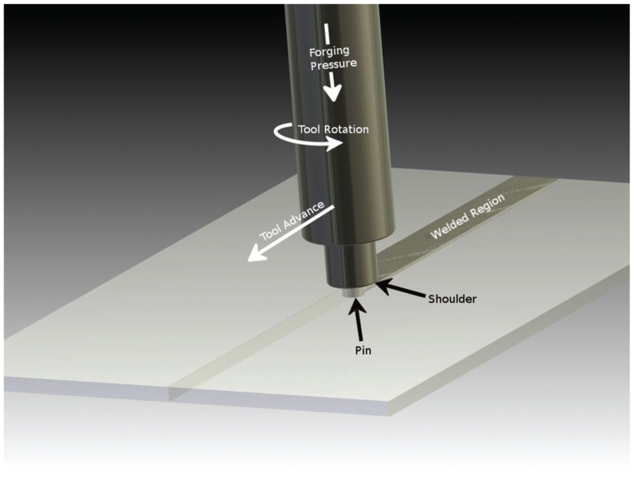
Illustration of the FSW process.

FSW’s solid-state nature results in multiple benefits over traditional fusion welding. Gibson et al. ³ summarized the advantages of FSW, which includes the following: the newly forged material does not experience problems with melting and solidification such as porosity, embrittlement, and cracking; joining at low temperatures results in lower distortion and lower residual stress; FSW is environmentally friendly due to the absence of filler material, fumes, arc flash, splatter, and the pollution associated with most fusion welders. FSW’s solid-state nature is advantageous for metal alloys with low melting points that typically have a high strength-to-weight ratio. The process results in increased mechanical properties with fewer defects. Because of the advantages of FSW, it is rapidly finding use in the marine, automotive, and aerospace industries and has resulted in the reduction of weight, number of parts, and manufacturing cost as well as increased joint strength of the welded material.^1,3

Despite the clear advantages of FSW over traditional fusion welding, problems can arise when improper FSW occurs. The process has led researchers to investigate why defects occur and how to detect them. The defects that can result during the FSW process include excessive flash, excessive concavity, tool particulate inclusions, foreign substances, entrapped oxide defects, voids, and wormholes. Gibson et al. ³ defined a wormhole as a void in the weld seam that forms under non-ideal welding conditions and that can reduce the structural quality of the weld and cannot always be visually spotted.

Because visual testing cannot always be used to spot flaws, other costly methods are employed to detect faults. Current post-weld, non-destructive testing includes radiographic testing, ultrasonic testing, phased array ultrasonic inspection, and laser ultrasonic testing. As an example of recent research, Kleiner and Bird ⁴ analyzed ultrasonic noise distributions collected during a weld with phased array equipment in order to detect entrapped oxide defects. Statistical signal processing algorithms were then developed, which gave a reliable reading of the quality of the FSW process analogous to the likelihood of entrapped oxide.

While these methods are state of the art, they cannot detect flaws in the weld until after the process has taken place. Current detection methods such as the ones mentioned above are both time-consuming and expensive; any flawed parts have to be scrapped. In addition to costly post-weld analysis, manufacturing is moving from mass production to small lot production. Examples can be seen in planes, cars, and rockets. When production volume is lower, it is more costly to manufacture and produce parts for testing and disposal. The proposed answer to small lot manufacturing is in-process monitoring and control in which the operator understands the process and can monitor and adjust parameters to prevent the formation of flaws. ⁵

Prior research has been conducted regarding methods for the in-process detection of FSW defects. A common method for predicting the quality of the weld is by examining the forces during welding. Fleming et al. ⁶ performed Fourier transforms on the force signals collected during welding with varying degrees of gap faults. Using statistical analysis, they were able to separate the faulty welds from the control welds. Burford et al. ⁷ were able to provide better detection capabilities than either x-ray or tensile testing through the use of a neural network algorithm applied to the transverse feedback forces. The neural network was trained using two feature vectors for each point of interest from the transverse force and a third to test the classification. When 100% of the feature vectors were used, 92.7% of the samples were correctly classified. Similarly, Boldsaikhan et al. ⁸ asserted that the oscillations of the feedback forces are related to the plasticized material flow, which enables to detect a void using the frequency spectrum. Using a discrete Fourier transform and a multilayer neural network on the frequency spectrum, bad welds were classified from good welds with a 95% success rate. Jene et al. ⁹ developed monitoring software, Monstir, to investigate how the welding parameters lead to oxide particle forming in the weld. Monstir uses statistical analysis of process parameters (feed per revolution, surface of the weld face, and periodical length of the welding force frequency) and welding forces to draw conclusions on the weld quality. In addition to finding that welding parameters influence oxide particle distribution, it was concluded that accurate validation of wormholes and the prediction of tool breakage were possible. Another in-process detection method, acoustic emission monitoring, was performed by Subramaniam et al. ¹⁰ on different tool geometries and analyzed with a fast Fourier transform. A correlation was made between different acoustic emissions and the tensile strength of a weld joint.

The work presented in this article examines the development of an automated process monitoring system for FSW. The system indirectly monitors the welding torque through the current supplied to the spindle motor. The decomposition of the current into its frequency spectrum is used to determine when a void is present during the welding environment. As mentioned previously, voids and wormholes are of great concern because they are not always visible and reduce the structural integrity of the weld.

Metal flow theory and experimental approach

Metal flow theory

Because the welding environment is beneath the shoulder of the tool, our understanding of metal flow is limited. Prior research by Schneider ¹¹ and Schneider et al. ¹² has presented a plausible model based on experimental research. In addition, Schneider et al. ¹² performed extensive trace experiments where lead wire was placed along the faying surface prior to welding. During the welding process, the tool stirred the lead wire into the weld seam. The flow of metal due to the stirring action was revealed through x-ray imaging of the weld seam. From this work, a model known as the Nunes kinematic model was later presented. ¹¹ This model presents a rotating plug of metal beneath the shoulder of the tool. The plug sticks to the surface of the tool and rotates within the workpiece. At the boundary between the rotating plug and the workpiece material is where the stirring action that forms the weld occurs. This boundary can be referred to as the shear interface boundary. It is the location within the welding environment beneath the tool’s shoulder where shearing of the material occurs continually. The shear stress from the applied (welding) torque at this interface surface equals or is greater than the shear flow strength of the material. Thus, plastic deformation occurs as the tool rotates.

Within the shear interface boundary, three flows are present:^11,12 a rotational motion around the tool, a translation motion through, and a ring vortex motion that provides vertical movement of the metal. These three flows combine to produce a net flow which tends to wipe the material around the tool where it is forged together on the backside of the tool due to the downward force of the tool’s shoulder.

As part of the metal flow model, oscillations are predicted in the size of the rotating plug beneath the tool. This is also referred to as oscillations in the slip–stick condition between the tool’s shoulder and the workpiece. If the shear flow strength of the workpiece is greater than the shear stress caused by friction from the tool’s shoulder at the workpiece’s surface at a given location beneath the tool, slippage occurs between the tool’s shoulder and the workpiece. If the shear stress from friction by the tool’s shoulder is greater than the shear flow strength of material, part of the material sticks to the tool’s shoulder and a shear plane or interface boundary is established below the tool’s shoulder.

This natural oscillation is necessary to provide a stabilization of the welding temperature and prevent melting of the parent materials. As plastic deformation occurs due to the shearing of the material, the temperature increases due to the mechanical work and energy release. This increase in temperature softens the workpiece and reduces the shear flow strength of the material. With the softening of the workpiece, the radius of the shear interface boundary is reduced. Shearing and plastic deformation takes place closer to the centerline of the tool. When this occurs, more slippage of the tool’s shoulder past the workpiece occurs. The heat generated from friction due to slippage is less than the heat released from the plastic deformation.

With a smaller shear interface boundary, less plastic deformation occurs, and less heat is generated. The reduction in temperature leads to a hardening of the material and an increase in the shear flow strength. The shear interface boundary migrates further from the tool’s centerline. As the shear interface boundary grows in size, more heat is generated due to plastic deformation. With the increase in heat, the material softens and the cycle of slip–stick continues and thereby stabilizes the temperature.

From the tracer experiments, Schneider et al. ¹² reported in their conclusions two types of fluctuations present in the welding environment. First, the lead tracers were dispersed (200/min) in the wake of the tool at a rate equal to the tool rotation. Second, lateral scattering of the tracers occurred in the tool’s wake at a much lower frequency than the tool’s rotation (20/min). The lateral scatter was believed to be a result of the oscillation in the size of the shear interface boundary. An increasing radius in the shear interface boundary holds the tracer element slightly longer and deposits it on the advancing side while a decreasing radius deposits the material sooner on the retreating side.

With the oscillation of the slip–stick condition, the welding torque will oscillate in conjunction. The welding torque as defined by Nunes et al. ¹³ is the summation of the torque acting at the shear interface boundary that surrounds the tool (see equation (1)). It sums the torque acting on the tool’s shoulder, side of the pin, and finally the bottom surface of the pin

$$\mathrm{Torque}=\underset{r}{\overset{R}{\int }}2\pi r^2\sigma \mathrm{dr}+2\pi r^{2}t\sigma +\underset{0}{\overset{r}{\int }}2\pi r^2\sigma \mathrm{dr}$$

(1)

Equation (1) approximates the size of the shear interface boundary as the surface area of the tool. The torque is determined using the shear flow stress acting at the shear interface boundary and its location. Because the shear interface boundary oscillates in size as described above, the welding torque will oscillate as well.

The oscillation of the slip–stick condition is supported by work from Qian et al. ¹⁴ Although the intent of their work was to determine the fraction of slip and sticking, they found a clear oscillation between the two conditions as well as torque. Their results showed the oscillation to be equal to the tool’s rotation rate.

Another study by Fonda et al. ¹⁵ found that consistent material flow patterns such as “onion rings” are a result of an off-centered tool. Periodic reversals of the shear plane were thought to create the microstructure patterns within the weld. The reversals in the shear plane and thus shear forces were also believed to be responsible for the typically observed oscillation in machine forces including the torque.

From the studies described above, the presence of a steady oscillation in welding torque exists during normal operations. Nunes et al. ¹³ predict it mathematically, while Schneider et al., ¹² Schneider, ¹¹ Qian et al., ¹⁴ and Fonda et al. ¹⁵ all found it to be present but with different explanations.

Experimental approach

From the prior research discussed above, a natural oscillation of the welding occurs. As noted in equation (1), the welding torque can be numerically predicted assuming that the shear interface boundary is continuous around the tool. When the shear interface boundary is continuous, the welding process will be in a steady-state condition. In addition, when the correct parameters of tool rotation rate, plunge depth, and speed are selected, a high-quality weld should be produced.

However, if a void or wormhole develops in the welding environment, the shear interface boundary will not be wrapped continuously around the tool as described by equation (1). The shear interface boundary will have pockets or holes in it. When these pockets appear, there should be a change in the frequency of the slip–stick condition.

As with any quality monitoring system, the desire is to monitor during the actual production operation and without affecting the production equipment. Prior research by Longhurst et al. ¹⁶ found that the welding torque could be controlled using the current supplied to the spindle motor as feedback. To obtain the feedback, they used an inexpensive clamp-on current meter to measure the spindle motor current. The current provided an indirect way of monitoring the welding torque. Furthermore, Mehta et al. ¹⁷ reported a similar method for measuring the torque and process forces during FSW by monitoring the input current to the motors.

The presented research used the same type of clamp-on current meter to perform process monitoring since the current signal provided an indirect measurement of the welding torque. The use of a clamp-on current sensor could be added to any existing FSW machine without interference to the production operation.

To examine the frequency spectrum, a Fourier transform was performed on the recorded current signal. The Fourier transform function decomposed the signal into various frequencies present in the welding environment and equipment. To create voids in the shear interface boundary and welding environment, holes were drilled in the faying surface prior to welding. The frequency was examined during the steady-state condition with no voids present and again when the voids were encountered.

The results show that a clear and distinguishable shift in the frequency spectrum occurs when voids are encountered. During normal welding (i.e. no void), a significant amount of signal content is present at 14 Hz for the experimental setup presented. When a void was encountered, the content at 14 Hz disappears, while sometimes, an increase in content is observed near the 1- to 4-Hz range. Although a thorough understanding of the frequency content is not complete, this change in content was repeatedly observed when a void was present.

Experimental setup

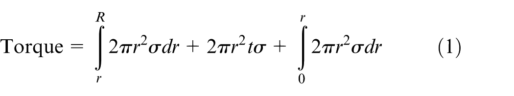
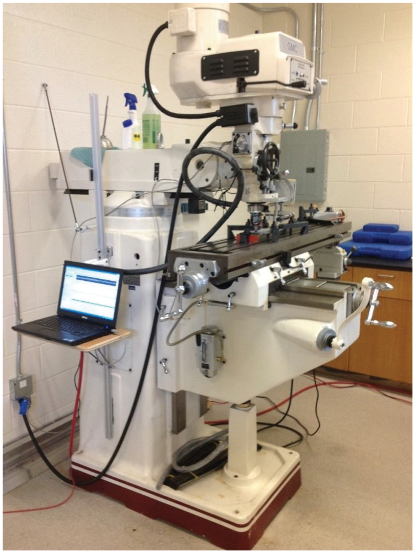
Experimental welding was conducted using a three-axis GMC milling machine with a 3-Horsepower spindle motor. The worktable had a power feed in the direction of welding. The milling machine was outfitted with sensors and a data acquisition system as shown in Figures 2–4. The sensors included strain gauges, a clamp-on current meter, and a potentiometer. For measuring the torque, a quantity of four, 350 Ω strain gauges (Vishay Micro-Measurements part number CEA-06-187UV-350) in a full Wheatstone bridge configuration were mounted to the tool holder (commonly referred to as an end mill holder when used during machining operations) which held the FSW tool via a set screw. The gauges were installed per the installation instructions from Vishay Micro-Measurements using their M-Bond 610 adhesive kit. To transmit and receive electrical signals from the rotating strain gauges, a Fabricast slip ring assembly (part number 1926-2BR-FAG180) was mounted to the spindle shaft exposed below the casting and just above the tool holder. A small circuit board was fabricated for conditioning and processing a 10-V signal through the strain gauge circuit. To measure the signal difference across the Wheatstone bridge, an instrumentation amplifier (analog devices AD624) was used. It obtained the voltage difference across the bridge and conditioned the signal before it was recorded. A gain of 1000 was selected and configured with the wiring of the AD624 instrumentation amplifier. For measuring the current, an NK Technologies (model number AT1-010-000-SP) clamp-on current meter was placed around one of the three wires supplying power to the spindle motor (see Figure 3). The clamp-on current meter has three input current ranges (0–10 A AC, 0–20 A AC, and 0–50 A AC) and a root mean square (RMS) output range of 0–10 V DC. For our research, the input setting was 0–10 A. For recording the FSW tool’s position along the weld seam, a UniMeasure string potentiometer (model number LX-PA-50) with an input of 10 V was used. To record the signals and convert them to their respective units, National Instruments (NI) Signal Express software was used in conjunction with an NI data acquisition device (DAQ; model number NI USB-6009). The DAQ was capable of handling the three analog inputs. A range of −1 to +1 V were used for the differential input of the signals from the strain gauges, while the current sensor and potentiometer each used a single-ended input with a range of 0–10 V. The DAQ had an input resolution of 14 bits and a sampling rate of 1000 Hz.

Figure 2.

Three-axis FSW machine.

Figure 3.

Clamp-on current sensor.

Figure 4.

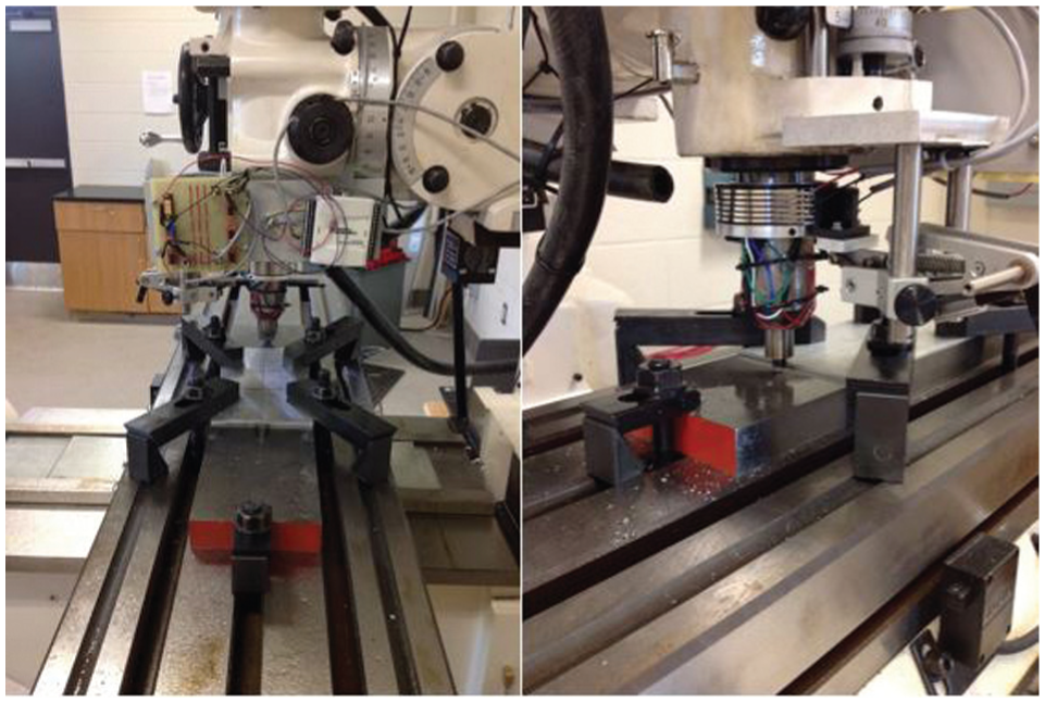
Sensor board, tool holder, strain gauges, and experimental setup.

Calibration of the strain gauges was performed by inserting a custom-made tool into the tool holder. The custom tool had a 6-in (15.25 cm) arm attached to its bottom that allowed a cable to be attached. From the end of the arm, the cable ran over a pulley that was attached to the end of the worktable. The pulley allowed for the suspension of weights over the edge of the table. The suspended weights in conjunction with the custom tool and its arm applied a known torque to the FSW tool holder. During calibration, the arm of the custom tool was placed at a 90° angle with the cable. This allowed for the easy determination of the torque (arm length multiplied by weight attached).

Masses of 1, 3, 5, 8, 10, and 15 kg were each suspended from the cable–pulley system, and the corresponding weights and torque were calculated. In addition, the output electrical potential (V) from the strain gauges was recorded for each of the applied loads. This process was repeated three times for both clockwise and counterclockwise torques. Plots of applied torque as a function of output voltage were created, and a best fit line was established. The calibration data and resulting best fit line between datasets showed a very linear and consistent relationship between applied torque and output voltage, thereby giving a reliable conversion between torque and voltage. The average applied torque per output voltage was 167.53 N m/V.

The weld samples were 1/8 in thick (3.175 mm) by 2 in wide (50.8 mm) by 8 in long (203.2 mm) aluminum 6061. To ensure voids were present in the welding environment, 1/16 in diameter (1.59 mm) holes were drilled to a depth of 1/16 in (1.59 mm) into the faying surface. Two holes were drilled along the faying surface so that during each weld, two voids would be encountered. The holes were placed 3 in (76.2 mm) from each end of the workpiece. The holes were present in both pieces to be joined. A prepared sample is shown in Figure 5. Additional samples were prepared with 0.040 in (1 mm) for comparison purposes.

Figure 5.

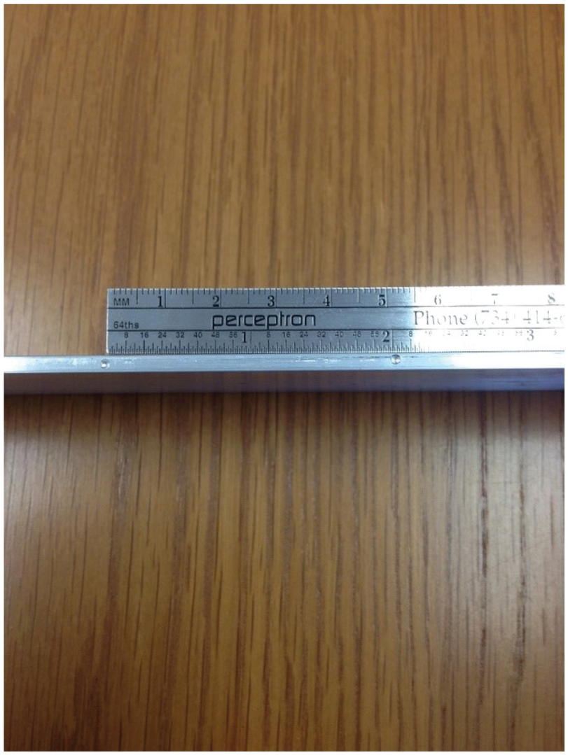
Workpiece prior to welding with voids (1.5 mm diameter) drilled into the faying surface.

The drilling of the holes into the faying surface was chosen to ensure the presence of voids in the welding environment without altering the process parameters. The drilling of holes simulates improper workpiece fit-up that is not visible by production operators. In addition, the drilling of the holes provides a known void size and location for comparison to the collected weld data. Creating voids by suddenly altering the process parameters was not chosen because it is not reliable and does not provide a controlled comparison to the collected weld data. Historically, process parameters have been kept constant during steady-state welding conditions.

The welding parameters selected for the tool were 1400 r/min, 2 in/min (50.8 mm/min), and a shoulder plunge depth of 0.003 in (0.0762 mm) for the trailing edge of the shoulder. The tool was placed on a 1° lead angle. FSW can be performed over a wide range of tool travel and rotation speeds. The selected parameters on the machine used for this experiment produced quality welds that were satisfactory. The machine was a small three-axis milling machine as described above and is shown in Figure 2. The selected process parameters also kept the process forces within safe limits so as not to damage the machine or risk injury to the operators. The goal of the experiment was not to optimize the process parameters to produce the highest strength weld.

Results and discussion

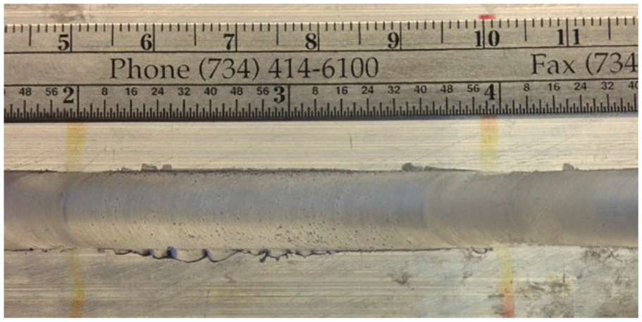
Approximately 20 weld samples were produced and examined. For each sample, the welding torque, spindle motor current, and the tool’s position along the weld seam were recorded. The welding tool entered one end of the weld sample and exited the other simply by running in and then out of the edges. A completed weld sample is shown in Figure 6. The red lines on top of the sample indicate where the holes were located within the faying surfaces. As viewed in Figure 6, the tool entered the left side of the weld sample, traversed 3 in (76.2 mm), and then encountered the first void. The second void was encountered after two additional inches (50.8 mm) of travel. Finally, the tool traveled 3 in (76.2 mm) and exited the right side of the workpiece.

Figure 6.

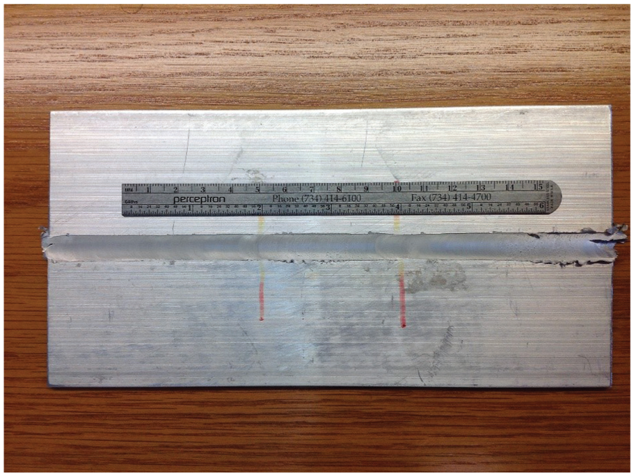
Welded sample.

On close inspection of the sample, one can see a slight disruption to the surface pattern in the vicinity of the voids. The surface pattern is created as the tool stirs and moves along the weld seam. This disturbance is due to the voids in the faying surface. However, because they are very slight, it is not easily distinguishable as a possible flaw; hence, it is desired to analyze the process data and use a less empirical method for distinguishing flaws.

All samples consistently produced the same results regarding torque and current patterns. Three samples are presented and discussed in detail below. Since the weld torque was measured via strain gauges and the electrical signal was passed through a rotating slip ring, a low-pass filter was used to reduce the electrical noise. The filter was part of a software feature in NI Signal Express.

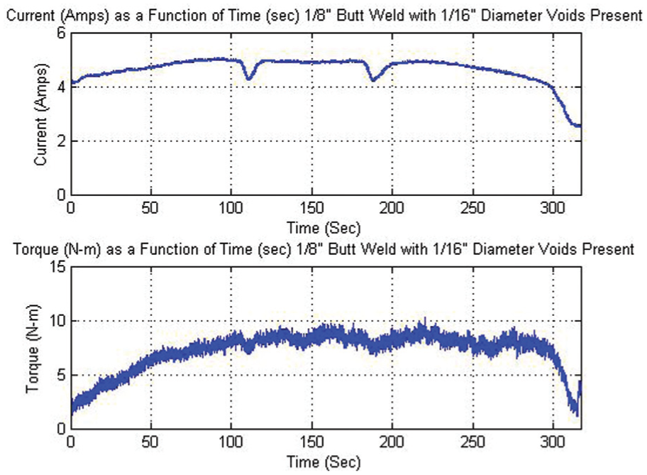
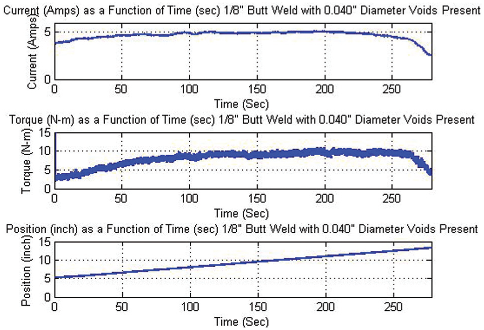
Figure 7 presents the torque and current from the first sample. For this particular weld, the low-pass filter in the Signal Express software was set at 20 Hz. Still with the filter, there was a significant amount of noise. However, it does appear to follow the same trend as the spindle motor current. The signal from the clamp-on current sensor provided a voltage that was much cleaner and free of the noise experienced in the strain gauge system. On inspection of the current, one can see that two dips occur in its magnitude at approximately the 80- and 150-s marks. This dip in the magnitude of the current is due to the tool encountering the void in the welding environment. Although much more difficult to distinguish, a slight disturbance is also visible in the torque signal at the corresponding times.

Figure 7.

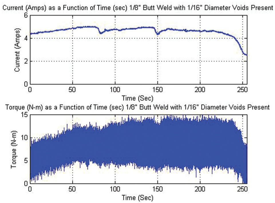
Plots of torque and current for sample 1.

Based on the results presented in Figure 7, if a process monitoring algorithm examined the current and alerted the operator each time the current exceeded an upper or lower limit, it would not be reliable because the current has a relatively large range during the welding process. If voids were present, as in the experiment, they more than likely will be within the upper and lower boundaries of the current during the welding operation. Hence, our research was to examine the frequency content of the current signal and see if it could provide a reliable means to detect voids.

To conduct this analysis, a MATLAB program was written using the fast Fourier transform command to calculate and plot the frequency content of the signal. Since the DAQ sampling rate was 1000 Hz, it was decided to examine the weld data in 1-s intervals. In other words, we took 1000 points of data at a time and determined the frequency content. Since the tool’s travel speed was approximately 2 in/min (50.8 mm/min), we concluded this was an appropriate block of data and time to examine. The tool’s travel speed equates to 0.03 in/s (0.85 mm/s). With a void diameter of 1/16 in (0.0625 in; 1.59 mm), the leading edge of the tool was estimated to be somewhere within the void for approximately 2 s. Thus, resolving the current signal into its frequency spectrum every second provided the appropriate resolution. For instance, if the tool was traveling at a faster rate, such as 4 in/min (101.6 mm/min), the calculation of the frequency content should be done for every half second of data. This would provide two datasets of frequency content where the tool’s edge was within the void. The void’s influence on the welding environment may be for a much longer period of time as it swept (or no material in this case) around the tool toward the tool’s backside according to the metal flow theory presented above.

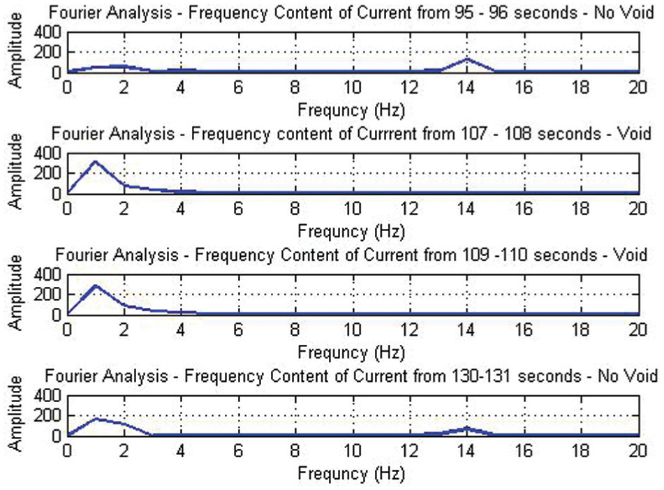
Figure 8 shows the frequency spectrum of the current before, during, and after the tool encounters a void during the first sample. Each sample has two voids in it; thus, Figure 8 presents the frequency spectrum surrounding the first void which was encountered near the 80-s mark. Prior to encountering the void, the frequency spectrum looks similar to that present at the 70- to 71-s mark. The frequency spectrum at this time is representative of each point of analysis where no void was present. The spectrum of frequency has content at approximately 1.5–2 and 14 Hz. This is also seen after the tool passes through the void, and normal welding conditions have returned near the 105- to 106-s mark. In contrast to regions where no void is present, the frequency spectrum is clearly different when a void is present. As can be viewed in Figure 8 at the times between 81 and 85 s, the frequency content increases in the region near 1–4 Hz and disappears at 14 Hz. The maximum amplitude is nearly doubled at 1.5 Hz when a void is present. When the entire weld seam was analyzed for frequency content, the voids appeared to be present or influencing the welding environment for 3–4 s each time. Thus, with voids influencing the welding environment for this duration, validation is obtained for the selection of 1 s intervals of data for frequency analysis. With the travel speed and void size, the 1-s interval of data analysis provided the appropriate resolution needed for void detection. In addition, with the void appearing to influence the welding environment for approximately 3–4 s, support is also given for the estimate of void contact and influence as discussed above.

Figure 8.

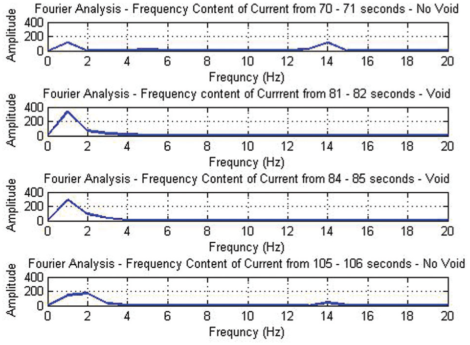
Frequency spectrum of the current as the tool encounters a void for sample 1.

In addition, the 3–4 s of detection also supports the hypothesis that the void and its influence is in the welding environment longer than just the time the leading edge is in contact with the void. As further evidence of the void’s influence, the length of the surface distortion (or change in surface pattern created by the rotating tool) seen in Figure 9 supports this as well. As can be seen in Figure 9, the distortion appears to the left of the red line where the void (hole) was wiped to the backside of the tool. In this area, the width of the weld seam is slightly narrower, and the surface markings are smoother. Each distortion is approximately 0.2–0.3 in (5–7 mm) in length although it is difficult to identify a distinct starting and ending point. The red line on the left side of Figure 9 is the location where the first void was located, while the red line on the right side is where the second void was located. A trained technician might be able to visually detect a change in the welding environment but only after the welding operation when the weld surface could be closely examined. However, the goal is to detect the flaw as it is occurring so that corrections can be made.

Figure 9.

Picture of surface pattern of the weld seam.

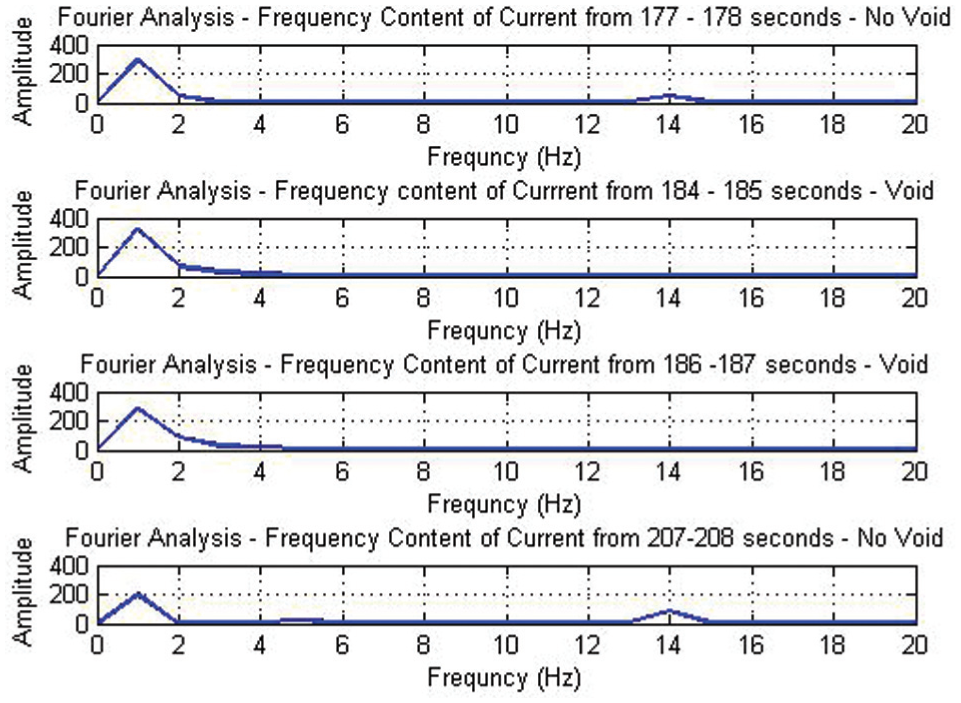
Data for the tool’s encounter with the second void in the sample are presented in Figure 10. The data presented in Figure 10 are strikingly similar to the data presented in Figure 8. As stated earlier, the entire weld seam was analyzed, and the frequency spectrum continually remained the same except for where a void was present. However, we did not analyze the starting and ending of the weld because the tool was running into and out of the sample’s edges. Each time a void was present, the frequency content disappeared at 14 Hz and increased in content within the 1- to 4-Hz range.

Figure 10.

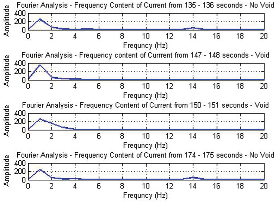
Frequency spectrum of the current as the tool encounters a second void for sample 1.

From Figure 10, one can see that when no void was present (before and after the tool encountered the void) near the 135- and 174-s marks, frequency content is present at 14 Hz. However, when the tool encounters the void between the 147- and 151-s marks, no frequency content is present at 14 Hz. This pattern as presented in Figures 8 and 10 was observed in the 20 weld samples produced.

To further illustrate the consistency of the observed pattern, data from a second sample are presented in Figures 11–13. Figure 11 presents the spindle motor current and welding torque. Once again, the current was obtained via the clamp-on meter, and the torque was acquired using the strain gauges that were mounted to the tool holder. For this second sample, a different cutoff frequency was selected for the filter within the NI Signal Express software. A cutoff frequency of 5 Hz provided a much easier graph to read than the one present in Figure 7.

Figure 11.

Plots of toque and current for sample 2.

Figure 12.

Frequency spectrum of the current as the tool encounters a void for sample 2.

Figure 13.

Frequency spectrum of the current as the tool encounters a second void for sample 2.

In Figure 11, we can see the two dips in the current near the 110- and 185-s marks. These dips are attributed to the voids created in the faying surface and encountered by the tool. In comparison with welding torque measured via the strain gauges, the voids are not clearly distinguishable. Several other dips occur in the welding torque. These might be associated with noise, but regardless, the voids cannot be distinguished. Thus, something other than torque must be used for the process monitoring.

Once again, using 1 s intervals of current data, frequency analysis was performed along the weld seam. The results are shown in Figures 12 and 13. These figures show that when a void is not present, there is frequency content at 14 Hz. However, when the void is in the welding environment beneath the tool, there is no frequency content at 14 Hz. It appears that within the frequency spectrum, content is shifted to a lower region. As observed in these figures, the content in the 1- to 4-Hz range increases when the void is present, while the content at 14 Hz disappears.

Finally, an attempt was made to determine the approximate resolution capability of this in-process monitoring method. Obviously, there is electrical noise inherent to all systems, and there is a limit to the sensitivity of the welding torque. For instance, as material is stirred by the tool, there will always be some type of microscopic areas of discontinuity that will be naturally present. This discontinuity will cause variations in the torque. Thus, if a void is small enough, its effect on the welding torque will be saturated within the normal variation of the signal.

To investigate this limitation, a weld sample with 0.040 in (1 mm) voids was examined. The same welding parameters were used as before. The results are shown in Figure 14. The smaller voids were not detectable as before when simply looking at the magnitude of the current or torque. To determine the time when the voids were encountered, we have to look at the position of the tool. The first void is 3 in (76.2 mm) from the end of the workpiece and the second void is 2 in (50.8 mm) past the first. The tool started at the 5-in mark, and thus, 3 in of travel (8 in position) is achieved near the 100-s mark. The tool travels the additional 2 in (10 in position) near the 160-s mark. Thus, the location of the first void is near the 100-s mark, while the second void is near the 160-s mark.

Figure 14.

Frequency spectrum of the current as the tool encounters a void for sample 3.

On completion of the Fourier analysis, no distinguishable shift could be found when the FSW tool encountered the void. However, the content of the signal at 14 Hz went to zero just prior to the 100-s mark, possibly detecting the void. The duration of no content was only for 1 s. This was unlike the detection of the 1/16-in-diameter voids where the content at 14 Hz disappeared for 3–4 s. The content never went to zero at 14 Hz near the second void at the 160-s mark.

Figure 15 compares the 14-Hz content of the current for the three weld samples discussed above. Recall that samples 1 and 2 had voids with a diameter of 1/16 in (1.59 mm), while sample 3 had a void with a diameter of 0.040 in (1 mm). On inspection of Figure 15 and the data for sample 1, one can see that the 14-Hz content clearly goes to zero near the 80- and 150-s marks. There are multiple data points where the amplitude is zero which clearly indicates a void. Similarly, the same condition exists for sample 2 near the 110- and 185-s marks. These are the points where the tool was in contact with the void. However, the detection of the smaller voids in sample 3 is not clear. The 14-Hz content goes to zero just prior to the 100-s mark, thus possibly indicating a void. However, the content clearly is non-zero near the 160-s mark.

Figure 15.

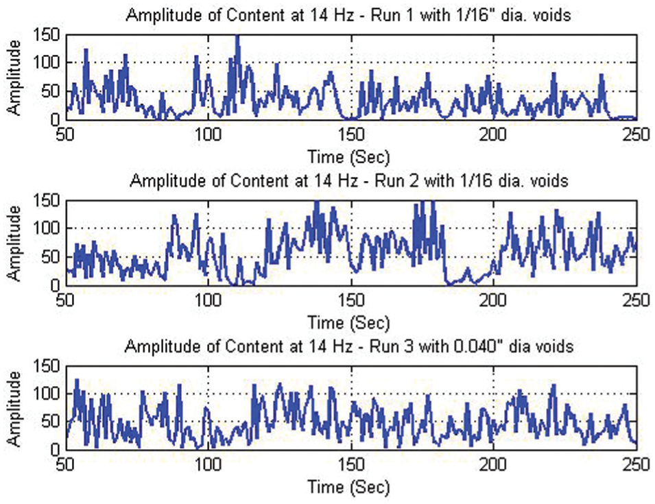
Content of the current signal at 14 Hz for weld samples 1, 2, and 3.

Conclusion

Using the spindle motor current to monitor the FSW process can potentially be a reliable technique. The results have shown that using a simple and inexpensive clamp-on current meter provides good insight into the welding torque. Using the clamp-on current meter, there is no interference with the existing equipment and process setup. In addition, the data are relatively free of noise as compared to the strain gauges and slip ring used for the experimental welding trials. For any existing production operation, a processing motoring system consisting of a clamp-on current meter, DAQ, and computer could be easily and inexpensively added. Finally, another advantage is the simplicity of monitoring a single-process variable rather than multiple variables.

The results consistently showed that when no void was present, there was a component of the current’s frequency at 14 Hz. However, when the tool encountered the void, the frequency spectrum changed. The component at 14 Hz went away while content in the range of 1–4 Hz increased. There was a desire to understand what was causing the current to have such a significant component at 14 Hz. The first thought was the tool’s rotational speed or imperfections with the alignment of the slip ring and its brushes. Neither of these proved to be the source. With the tool rotating at 1400 r/min, this equates to 23 Hz. If the slip ring and its brushes were producing the 14-Hz content, we would still see it when a void was present. Thus, it is probable that the 14-Hz content is related to the process and not related to the equipment.

The results also showed that this technique does have limitations. It can be concluded that the resolution for our setup was fine enough to detect voids of 1/16 in (1.59 mm) in diameter consistently but was inconclusive for voids of 0.040 in (1 mm) in diameter. With the larger voids, their presence was indirectly observed in the current amplitude as well as the frequency spectrum. However, for the smaller voids, the presence could not be observed from the amplitude alone. In addition, the frequency analysis was inconsistent and not reliable. In other words, this method of monitoring, similar to all systems, has its resolution limits.

Future work

Future work can be directed toward expanding the current setup to include welding trials over a range of process parameters as well as different tool sizes and designs. If the results are the same, this will give greater validity to this monitoring technique. In addition, effort should be directed to obtain greater resolution. Perhaps, this can be obtained by monitoring additional signals or creating a tool design that is more sensitive to the welding torque.

Effort should also be undertaken to obtain greater understanding of the welding environment. Specifically, effort should be undertaken to understand why the frequency spectrum of the motor’s current is distributed in the manner presented, and more importantly, it changes in the presence of voids. Deeper understanding of the welding environment will ultimately help develop better process control and monitoring techniques.