
Abstract
To improve the accuracy, generality and convergence of thermal error compensation model based on traditional neural networks, a genetic algorithm was proposed to optimize the number of the nodes in the hidden layer, the weights and the thresholds of the traditional neural network by considering the shortcomings of the traditional neural networks which converged slowly and was easy to fall into local minima. Subsequently, the grey cluster grouping and statistical correlation analysis were proposed to group temperature variables and select thermal sensitive points. Then, the thermal error models of the high-speed spindle system were proposed based on the back propagation and genetic algorithm–back propagation neural networks with practical thermal error sample data. Moreover, thermal error compensation equations of three directions and compensation strategy were presented, considering thermal elongation and radial tilt angles. Finally, the real-time thermal error compensation was implemented on the jig borer’s high-speed spindle system. The results showed that genetic algorithm–back propagation models showed its effectiveness in quickly solving the global minimum searching problem with perfect convergence and robustness under different working conditions. In addition, the spindle thermal error compensation method based on the genetic algorithm–back propagation neural network can improve the jig borer’s machining accuracy effectively. The results of thermal error compensation showed that the axial accuracy was improved by 85% after error compensation, and the axial maximum error decreased from 39 to 3.6 µm. Moreover, the X/Y-direction accuracy can reach up to 82% and 85%, respectively, which demonstrated the effectiveness of the proposed methodology of measuring, modeling and compensating.
Keywords
Introduction
High-speed and high-precision machining is an important development direction of modern manufacturing industry, and the application of high-speed spindle systems is crucial for the implementation of high-speed and high-precision machining. However, in order to improve the transmission performance, the built-in motor and high-speed bearings take the place of gearbox box, belt drive and so on, introducing a large amount of heat into high-speed spindle systems. In addition, the coupling of heat resource’s location and intensity, the heat dissipation, the spindle structure and the material properties also leads to complex thermal characteristics of high-speed spindle systems. Thermal errors caused by the uneven distribution of the temperature field are the most significant factors influencing the machining accuracy of computer numerical control (CNC) machine tools and account for about 70% of total errors resulting from various errors, and the more sophisticated the machine tool, the greater the proportion of thermal errors.1–3 Besides, the mapping relationship between thermal error and temperature field distribution is strongly nonlinear, resulting in the difficulty in thermal error modeling and compensating. Thus, eliminating thermal error of high-speed spindle systems is an effective way to improve the machining accuracy of CNC machine tools.
It is scholars’ lifelong pursuit to improve the machining accuracy of CNC machine tools by compensating thermal error. To study the thermal error modeling and compensation methods, the jig borer’s thermal drifts and temperature field distribution should be measured as accurate as possible However, the axial thermal expansion of the spindle system is measured by most of the researchers, while the measuring, modeling and compensation of radial thermal tilt errors is ignored. In fact, the radial thermal error of high-speed spindle cannot be ignored in terms of precision and ultra-precision machine tools. In this article, five eddy-current sensors were used to acquire thermal expansion and thermal tilt angles synchronously, and the thermal error models were developed based on artificial neural networks (ANNs).
In the past few decades, the modeling methods of thermal error of high-speed spindle systems had been studied, namely, the modeling method based on thermal characteristic simulation and the modeling method based on thermal characteristic experiments and engineering experience. In fact, thermal-induced errors could be reduced by optimizing the design of the machine tool structure at the design stage. However, the improvement of machining accuracy is just in a small limited range and the cost is relatively high. In recent years, numerical simulation methods based on heat generation and heat transfer have become a topic of increasing interest and are applied to analyze the distribution of temperature field and the variation of thermal errors of machine tools, and the most typical approaches are the theory of finite difference method (FDM) and finite element method (FEM). Bossmanns and Tu 4 applied FDM to describe the energy distribution, heat generation and heat dissipation of high-speed spindles. Zhao et al. 5 simulated the distribution of temperature field and thermal deformation of spindles based on Fourier’s law and Newton’s cooling laws using FEM. Creighton et al. 6 studied the thermal characteristics of micro-grinding spindle under varying spindle speeds using FEM. Lin et al. 7 presented a comprehensive model which considered thermodynamic characteristics of spindles to study their high-speed machining performance. Sukaylo et al. 8 presented an FEM-based computer model for the simulation of thermal deformation in multipass turning when different cooling conditions were applied. Xiang et al. 9 proposed a finite element model to optimize the thermal characteristic of spindle systems. However, heat generation and heat transfer were regarded as important boundary conditions in the above numerical models, which were difficult to be determined, resulting in a lower accuracy of simulation results and poor generality. Besides, the establishment of the thermal equilibrium equation is difficult for each node.
When it was difficult to establish the thermal characteristic analysis model of machine tools based on numerical simulation methods, scholars found that the thermal error compensation method based on thermal characteristic experiments and engineering experience is another more effective and economical method to improve the machining accuracy of CNC machine tools, especially for some less accurate machine tools which cannot be replaced immediately. So it is essential to study the systematic thermal error measuring, modeling and compensating methods of high-speed spindles. Moreover, thermal error models with higher accuracy, strong robustness and good convergence play the most important role in the compensation system.
Multiple linear regression analysis (MLRA) was widely used to construct the linear mapping relationships between temperature variables and thermal errors because it consumed less computer source in the compensation process.9–11 Time series model is also widely used in thermal error compensation systems due to its high accuracy and fast calculation.11,12 Postlethwaite et al. described a novel indirect measurement–based thermal error compensation technique that avoided the main difficulties of applying thermal compensation, making it practical and generally applicable. The technique made extensive use of thermal imaging for rapid assessment of machine tool thermal behavior and off-line development of the compensation models. 13 Lin et al. 14 and Zhao et al. 15 constructed thermal error compensation models based on support vector machine methods. However, only the axial thermal elongation was considered and the radial thermal tilt error was ignored in above thermal error compensation models. And the fact is that the radial thermal tilt angle errors have a significant influence on the terminal machining accuracy for the precision and ultra-precision machine tools. Therefore, the radial tilt angles should be considered in the thermal error compensation of spindle systems. Numerous studies showed that the relationship between the thermal error and temperature field was nonlinear. Therefore, different types of ANNs were widely used in thermal error compensation systems.11,16 And the results showed that the neural network with back propagation (BP) algorithm had a higher accuracy in data fitting than other modeling methods. However, the modeling method based on BP neural networks was easy to fall into the local minima, and the convergence performance of its multi-peak value was very poor, so the accuracy, convergence and robustness of the thermal error compensation models based on BP neural networks are not high. Moreover, BP neural network is a kind of algorithm based on gradient, so the convergence rate is slow. Moreover, it is difficult to determine the topology of the BP neural network. In fact, the determination of the number of nodes in hidden layers, the weights and the thresholds are usually based on experience of the scholars’ repeated experiments instead of theoretical guidance, resulting in the dependence of model’s accuracy, convergence and generality on researchers’ experience. On the other hand, the genetic algorithm (GA), which was efficient and robust at global searching, can be used to accelerate the convergence rate and improve the robustness and prediction accuracy of the traditional BP neural networks. Therefore, the combination algorithm of GA and BP modeling methods was proposed in this article, where a GA was used to optimize the number of the nodes in the hidden layers and the corresponding weights and thresholds of traditional BP neural networks.
The framework of this article is arranged as follows. Section “Thermal characteristic experiments” introduces the experimental setup and measuring principles, designs thermal characteristics experiments and analyzes the experimental results. A large number of temperature sensors and five eddy-current sensors were mounted to synchronously collect the temperature field and thermal drifts of the high-speed spindle system. Section “Grey cluster grouping and optimization thermal sensitive points” proposes the method of combining grey cluster grouping and statistical correlation analysis to group and select the typical temperature variables sensitive to the thermal errors. Section “Thermal error modeling and prediction” proposes a thermal error model based on the modeling principle of the traditional BP neural networks. Then an improved model, which is the combination algorithm of a GA and BP neural network modeling method, is used to optimize the number of nodes in the hidden layer, the initial weights and the thresholds of the BP neural network until these values meet the accuracy requirements. And the thermal error models, which considered the radial thermal tilt angles of the high-speed spindle system, were developed based on BP and GA-BP neural networks, respectively. Then, the thermal errors and temperature under different working conditions were used to validate the generality and robustness of thermal error models, and the predictive goodness and convergence of the thermal error models based on BP and GA-BP neural networks were compared. And the spindle thermal error compensation considering the thermal tilt angles is implemented on the jig borer spindle, and the compensative capacity of the two models was analyzed in section “Thermal error compensation.” Section “Conclusion” presents the conclusion obtained from previous analysis.
Thermal characteristic experiments
Experimental setup and measuring principles
Experimental setup
Thermal characteristic experiments were conducted on the high-speed spindle system of a jig borer for about 3 months to compare the accuracy, robustness and convergence of the two thermal error modeling and compensating methods based on BP and GA-BP neural networks.
The measurement system was developed based on American National Instrument NI-SCXI-1600. And it was applied to simultaneously acquire the temperature field distribution and thermal drifts of the high-speed spindle system. The temperature sensors (PT100) and five eddy-current sensors were used to acquire the distribution of the temperature field and the variation of thermal errors, respectively. Moreover, temperature and thermal errors were measured synchronously. And the temperatures and thermal errors were monitored in the experiments every 1 s. The mounting positions of the temperature sensors are as follows: rear bearing (T1), spindle pedestal (T2), the coolant outlet of the rear bearing (T3), the coolant outlet of the front bearing (T4), ambient (T5), front bearing oriented X− (T6), front bearing oriented Y+ (T7), motor oriented Y+ (T8), coolant inlet (T9) and coolant outlet of the motor (T10) and motor oriented X− (T11). And the mounting positions of the eddy-current sensors are as follows: radial near X-axis (S1), radial distal X-axis (S3), radial near Y-axis (S2), radial distal Y-axis (S4) and Z-axial direction (S5).
Measuring principle
Five eddy-current sensors were used to collect the thermal drifts of the spindle system according to Lin et al.
14
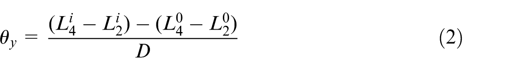
It can be seen that the thermal elongation E of the spindle can be collected by the eddy-current sensor S5. And radial thermal tilt angles
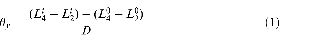
where i denotes the number of measurements,
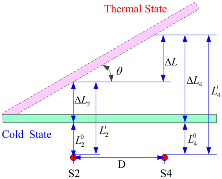
The spindle thermal inclination sketch.
Correspondingly, the thermal yaw angle
Experimental results and analysis
The rotational speed of the spindle system has great influence on the temperature distribution and the magnitude of thermal drifts. Therefore, the rotational speed distribution should be reasonably designed to simulate the actual machining process, as shown in Figure 2(a).
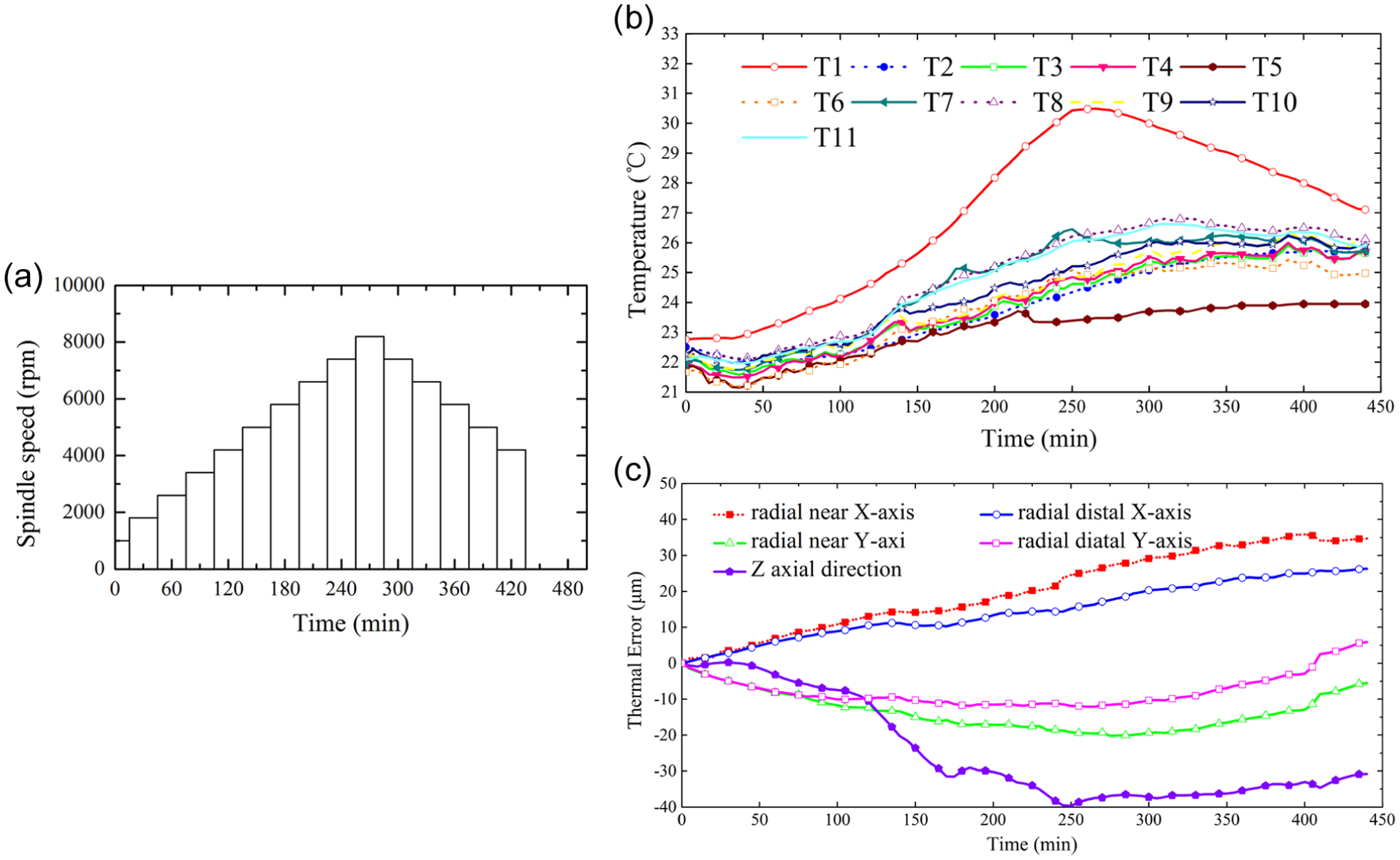
Thermal characteristic measurement: (a) step speed distribution, (b) temperature distribution and (c) thermal drifts.
Temperature field analysis
The variation of spindle temperature field with time is shown in Figure 2(b). It can be seen that the temperature curve’s slope varies with time because the heat generation of the built-in motor and the front and rear bearings changes with time caused by the change of the rotational speed of the spindle. Therefore, the change rates of the temperature curves exhibit fluctuation with time. It takes about 400 min for the spindle system to reach a thermal equilibrium state, and the temperature of the rear bearing is the highest among above measurement points because a large amount of heat is generated by the friction between the rolling elements and bearing rings and the heat dissipation condition of the bearings is poor. Moreover, the time to reach thermal equilibrium state is slightly different for different components of the spindle system because the heat capacity of the each component is different.
High-speed spindle systems are different from traditional mechanical spindles. And the power loss of the built-in motor and friction between rolling elements and bearing rings introduce a large amount of heat into the high-speed spindle system. Although a large amount heat could be removed by the cooling system, the heat generated by the built-in motor and bearings is still more than that removed by the cooling system. Therefore, the overall temperature increases with time in the first 270 min. And the temperature starts to decrease when the maximum of the rotational speed is reached because the heat generated by the built-in motor and bearings is smaller than the heat removed by the cooling system. Moreover, the temperatures of the bearings and the motor can be controlled in a limited range because the cooling system removed most of the heat. In addition, the temperature curves show a downward trend in the first 40 min because the heat dissipated by the cooling system is more than the heat generated by the built-in motor and high-speed bearings. In fact, the working cycle of the cooling system is that when the temperature of the spindle is higher than the threshold value, the cooling system starts to work.
Thermal error analysis
Figure 2(c) depicts the thermal drifts of the high-speed spindle. It can be seen that the thermal drifts increase with time until the maximum value is reached. And the thermal yaw
Grey cluster grouping and optimization thermal sensitive points
Grey cluster grouping and correlation analysis are adopted when experimental data of the typical temperature variables are grouped and selected to seeking the relationships among all the temperature variables to exclude multicollinearity and improve the robustness and precision of thermal error models. Subsequently, the key influencing factors on CNC machine tool’s spindle thermal errors can be obtained. The temperature variables are grouped by calculating the grey coefficient degree among temperature variables and then statistical correlation analysis is applied to calculate the grey correlation coefficient between each temperature variable and thermal error. Moreover, the temperature variable with larger correlation coefficient in each group is taken as the typical temperature variables. And the correlation coefficients and multiple correlation coefficients between each temperature variable combination and thermal error can be obtained, and the temperature variable combination with larger correlation coefficients and multiple correlation coefficients is taken as the typical temperature variable combination.
Grey cluster grouping
Grey cluster grouping is used to seek the relationship between each temperature variable and thermal error to identify the temperature variables which have greater impact on thermal errors. Assuming T = {T1, T2, …, Tn} is the temperature variables to be classified by grey cluster grouping.
In order to eliminate the coupling factor among the temperature variables, the temperature variables should be processed as the dimensionless quantity:
1. Initial value processing approach
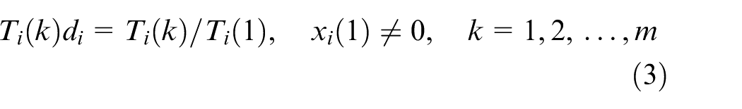
where Ti(k) denotes the kth sampling data of the ith temperature variable, Ti(1) denotes the first sampling data of the ith temperature variable, m denotes the number of sampling data and Ti(k)di denotes the dimensionless data of the ith temperature variable.
2. Equalization processing approach
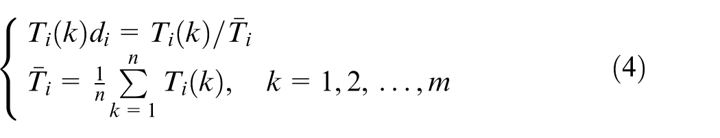
where
3. Interval-valued processing approach
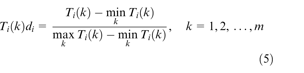
where
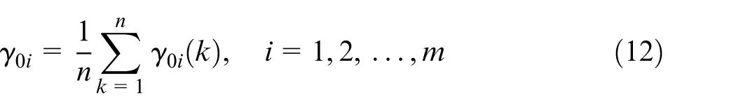
1. Grey absolute correlation degree. The temperature variables are processed as the dimensionless quantities by initial value processing approach and the grey absolute correlation degree
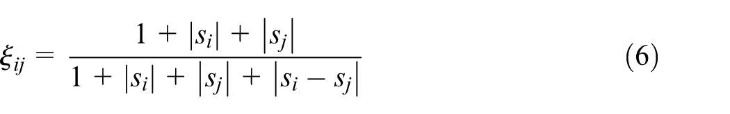
where
2. Grey relative correlation degree. The temperature variables are processed as the dimensionless quantities by equalization processing approach and the grey relative correlation degree
where
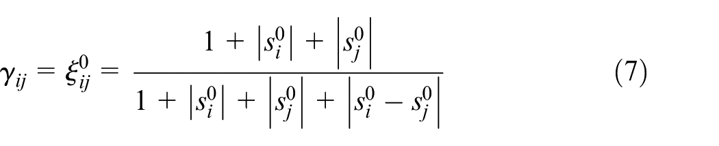
3. Grey comprehensive correlation degree. The temperature variables are processed as the dimensionless quantities by interval-valued processing approach and the grey comprehensive correlation degree

where
It can be seen from equation (8) that the grey comprehensive correlation degree is the combination of the grey absolute correlation degree and grey relative correlation degree, so it can reflect the similarity between two temperature variables and the change rate with respect to the starting point more effectively. Therefore, the grey comprehensive correlation degree can reflect the correlation between temperature variables Ti and Tj more effectively. The grey comprehensive correlation degree among the temperature variables can be obtained
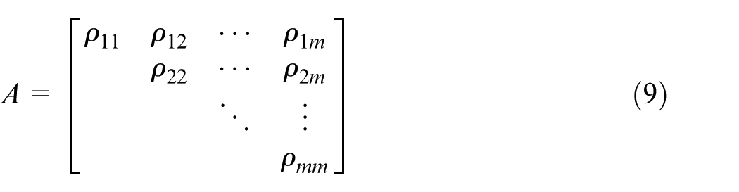
where
The greater the grey correlation degree

The grey comprehensive correlation degrees among temperature variables can be obtained when the significance level is
The grey correlation comprehensive degrees among temperature variables when the significance level is 0.9.
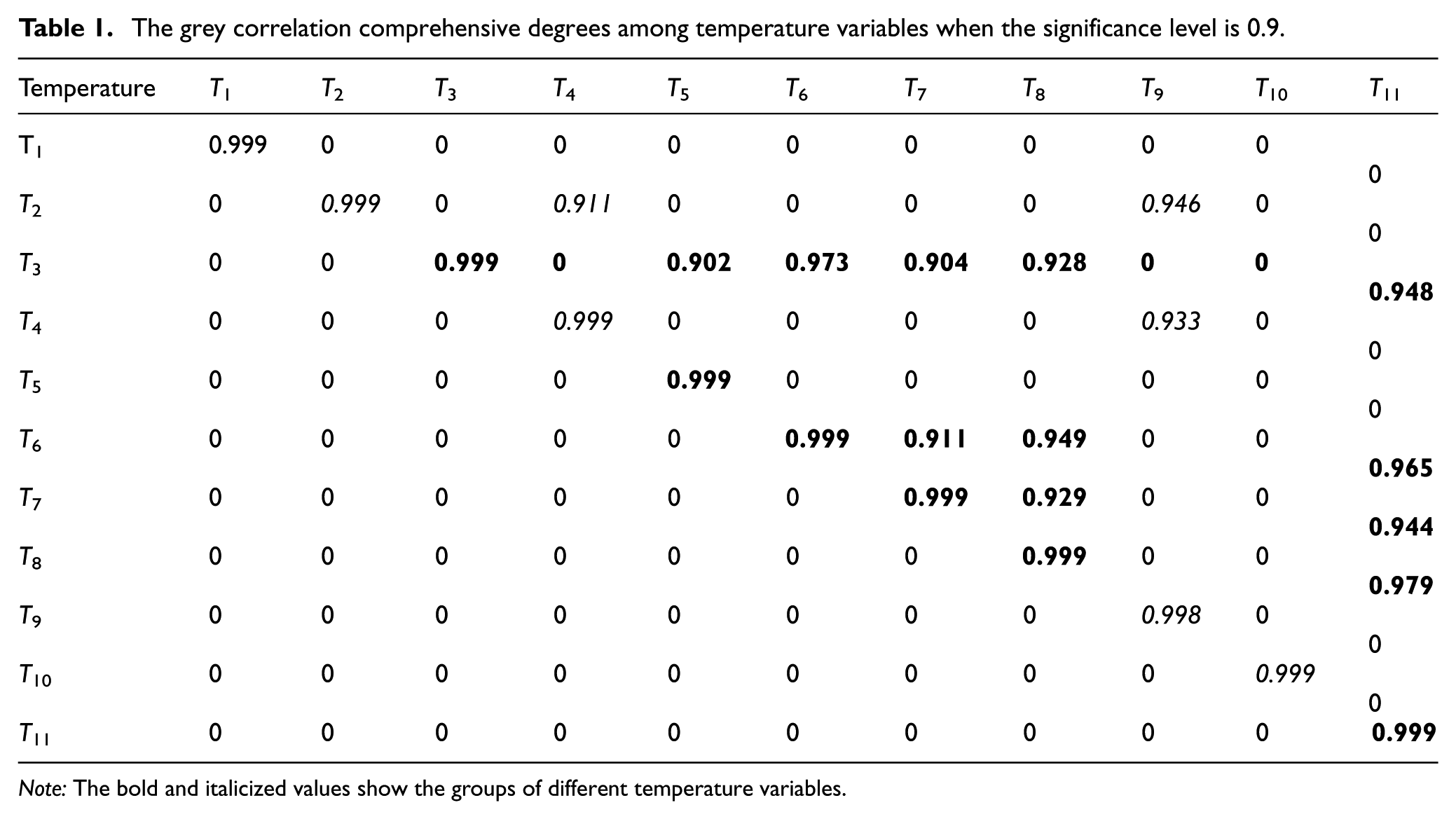
Note: The bold and italicized values show the groups of different temperature variables.
Optimization of thermal sensitive points
The temperature variables T = {T1, T2, …, Tm} and thermal errors S = {E,
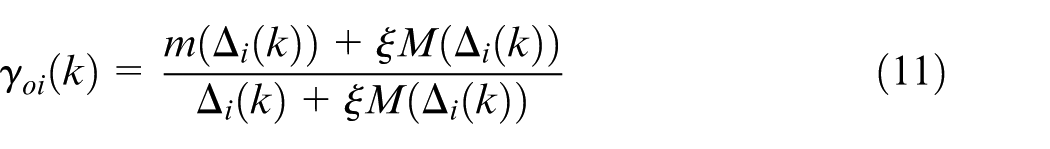
where
Grey correlation coefficient between axial thermal elongation E and temperature variables Ti.
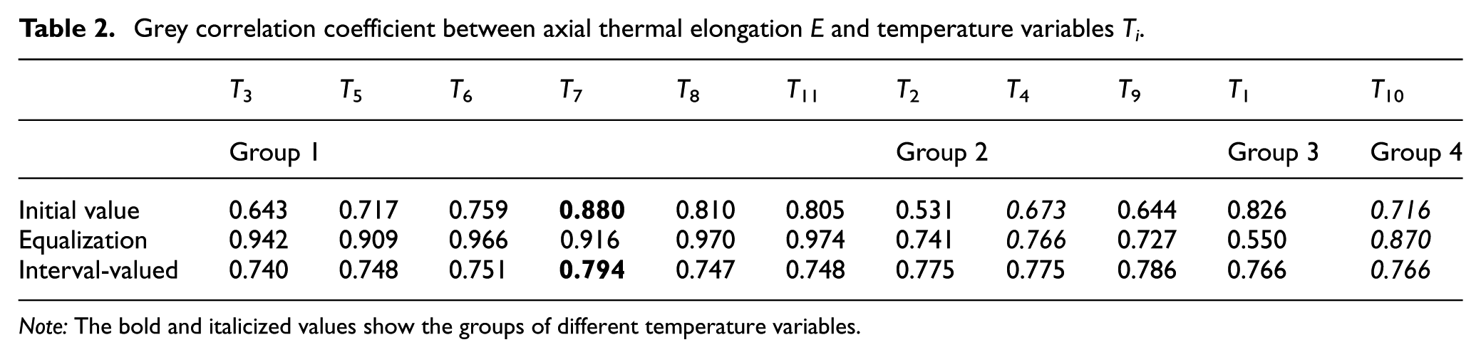
Note: The bold and italicized values show the groups of different temperature variables
Then, the grey correlation between E and Ti can be expressed as
The grey correlation coefficient between E and Ti can be obtained, as shown in Table 2. Combining the data shown in Table 2, T1, T4, T7 and T10 are selected as the typical temperature variables.
Selection of the optimal variable combination
Four temperature variables (T1, T4, T7 and T10) are selected as the typical temperature variables according to the above analysis. And the combination of the typical variables (T1, T4, T7 and T10) is conducted and there are 24-1 temperature variable combinations. Moreover, the correlation coefficients and multiple correlation coefficients between each temperature variable combination and thermal error can be obtained. The correlation coefficients represent the magnitude of the linear correlation between each thermal error and temperature variable combination. Assuming that the thermal error can be expressed as y, and its mean value is
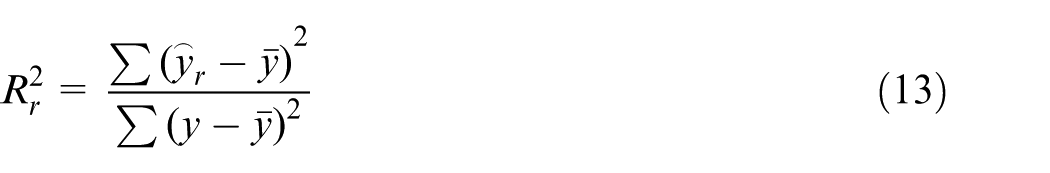
Then, the multiple correlation coefficients between thermal error y and temperature variable combination (T1, T4, T7 and T10) can be obtained
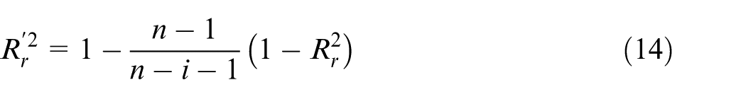
where n denotes the number of measurements and i denotes the number of the temperature variable combination.
The greater the correlation coefficient
Performance comparison of BP and GA-BP networks.
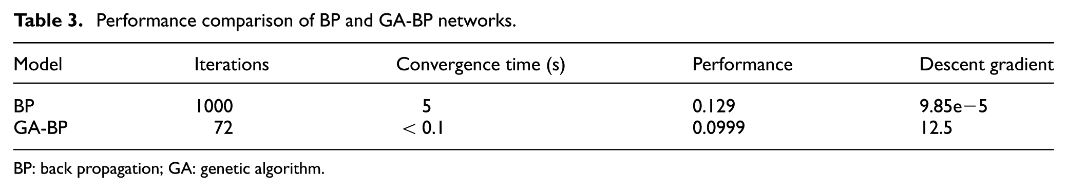
BP: back propagation; GA: genetic algorithm.
Thermal error modeling and prediction
BP neural network modeling
The BP network constituted by multi-layer neurons with error BP algorithm is the most widely used neural network. 18 It has good data parallel processing capability, excellent fault tolerance and superior nonlinear mapping features. 19 So it is reasonable to use the BP network to construct the nonlinear mapping relationship between thermal errors and temperature variables.
Assuming that

where
GA-BP network modeling
Integration of GA and BP algorithm
BP network is a kind of algorithm based on gradient, 20 so the convergence rate is slow. And it is easy to fall into the local extreme points, resulting in a lower accuracy of thermal error models. Moreover, the topology, the weights and thresholds are usually based on experience or repeated experiments instead of theoretical guidance, resulting in the accuracy and generality of the thermal error model dependent on the experience of researchers. 19 On the other hand, the global solution can be quickly searched by a GA in the whole solution space, and the whole searching space can be automatically obtained by GA. 21 In addition, it is difficult to fall into the local optimal solution because the rapid decline and its inherent parallel processing performance can be used to accelerate the convergence rate of the BP network.22,23 Therefore, GA can be used to globally search the number of the nodes in the hidden layer and the weights and thresholds of the traditional BP network to improve the accuracy, convergence and robustness of thermal error compensation model.
Assuming that the number of the nodes in the input, hidden and output layers are m, n and q, respectively, as shown in Figure 3, then, the number of the connection weights wji from the input layer to the hidden layer is
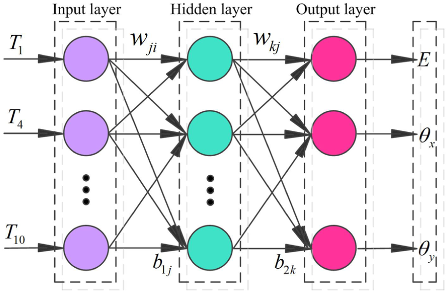
BP neural network.
The optimization process of the BP network using the GA includes three main parts: determination of the BP network structure, GA optimization and BP network prediction. The optimization of the topology, the connection weights and thresholds of the neural network are processed as follows:
1. Determine the input and output of the BP network. The typical temperature variables
2. Determine the coding method. An original generation is produced by coding the number of nodes in the hidden layer, the initial weights and thresholds of the BP neural network as parameters. Since the training process of the BP network is a continuous parameter optimization problem, real numbers are adopted as the coding contents.
3. Optimize the topology, the weights and thresholds of the BP network based on the GA. On one hand, the GA is employed to determine the number of the nodes in the hidden layer of the BP network. The reciprocal of the absolute value of the difference between the predicted and expected outputs of the BP network is regarded as the individual’s fitness function. The number of nodes in the hidden layer can be determined by performing such operations of GAs as the selection, crossover and mutation, as shown in equation (16)
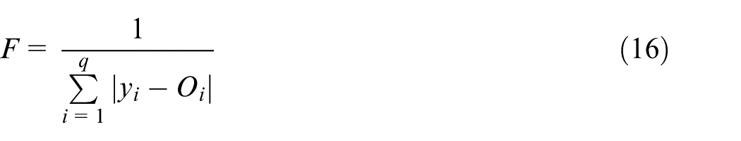
where q denotes the number of the nodes in the output layer, yi and Qi represent the predicted and expected outputs of the ith node, respectively.
The individual’s fitness value can be obtained by performing the operations of GAs. And the best individual can be selected among those individuals. Then, the number of the nodes in the hidden layer can be obtained by decoding the best individual.
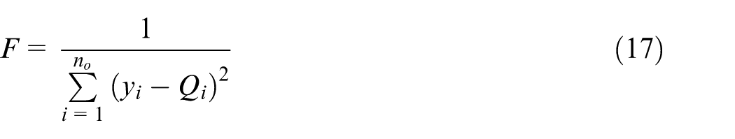
The individual’s length of the GA can be obtained after the topology of the BP neural network is determined. The reciprocal of the sum square of the difference between the predicted and expected outputs of individuals is regarded as the fitness function. The initial parameters of the BP network are optimized by setting the control parameters of the GA
The roulette method is adopted as the selection strategy. The larger the individual’s fitness value, the greater the probability being selected will be. And the crossover operator of the GA is a single-point crossover approach. In other words, two individuals are selected from the group based on a crossover probability, and parts of the two individual’s codes are exchanged. The mutation individuals are selected according to the mutation probability and the mutation position is randomly determined. Then, the GA is used to optimize the weights and thresholds until the best individual is obtained.
4. Predict thermal errors of high-speed spindle system based on the GA-BP network. The optimal predictive model for the high-speed’s thermal error can be obtained when the topology and the initial value of the BP network are determined. The sampling data are imported to train the GA-BP model and different sampling data are used to validate the effectiveness of the GA-BP model. And the performance of the GA-BP network can be evaluated by analyzing the value of the residual.
Topology of BP network
In section “Grey cluster grouping and optimization thermal sensitive points,” four typical temperature variables (T1, T4, T7 and T10) are selected as the inputs of the GA-BP model. The thermal errors, including E,
Parameters of GA
Real numbers are selected to form the GA structure, in which each weight and threshold of the BP network make up a chromosome string. There are a total of 100(4 × 10 + 10 × 3) connection weights and 10(10 + 3) thresholds to be determined because the topology of the BP network is 4-10-3, that is, the length of a chromosome string is 110(70 + 13). The fitness function is the same as equation (17). By this integration, global optimization and quick computation can be achieved at the same time.
Thermal error modeling
Models prediction and comparison
The thermal error compensation models based on BP and GA-BP neural networks are established, respectively. And the four typical temperature variables are regarded as input parameters of the BP and GA-BP neural networks and the thermal errors, including E,
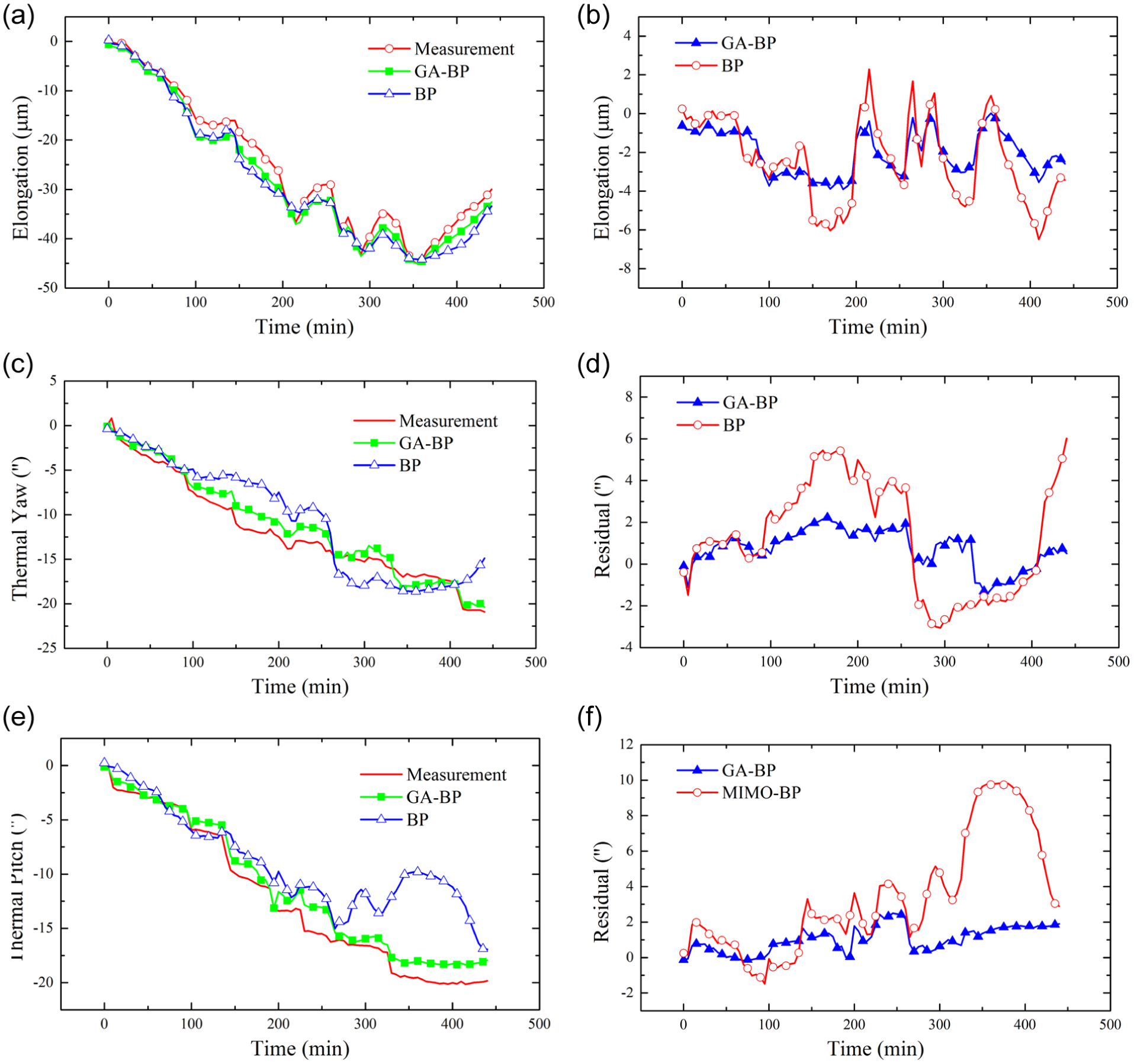
Regarding the data shown in Figure 2 as the training samples, the thermal error models based on BP and GA-BP neural networks are applied to estimate thermal errors. The comparisons of the fitting curves and the actual measurement are shown in Figure 4.
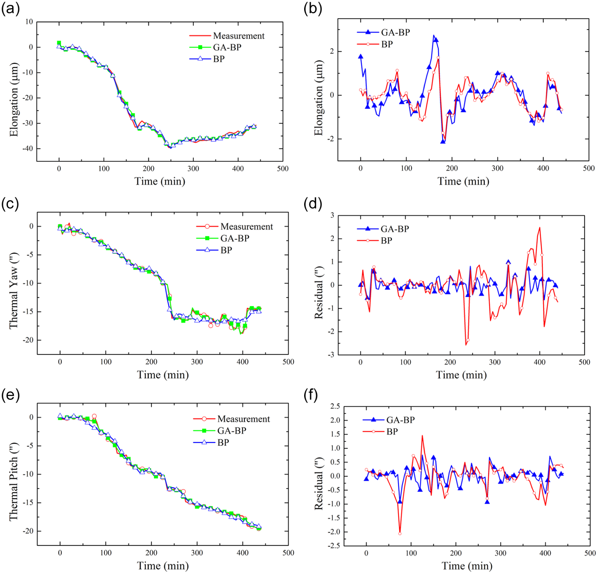
Comparison between estimation and measurement of original data: (a) estimation and measurement of thermal expansion, (b) residual of thermal expansion, (c) estimation and measurement of thermal yaw angle, (d) residual of thermal yaw angle, (e) estimation and measurement of thermal pitch angle and (f) residual of thermal pitch angle.
Then, the evaluation criteria of the model fitting are established. The absolute value


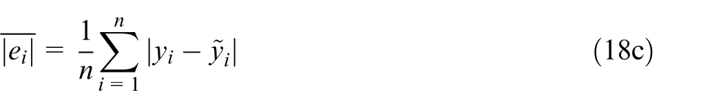
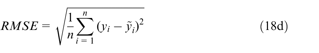
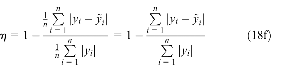
where
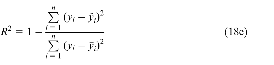
Then, the coefficient of determination R2 can be computed, and it can be used to characterize the extent to which the original data fall within the curve at a certain confidence level. The absolute mean values of the residual error of the two models are all small, and the RMSEs are similar which are close to zero, the coefficients of determination R2 are also close to 1. In addition, the predictive ability of the GA-BP model in three different directions are more than 97%, which indicates that the model has a higher predictive accuracy and fitting ability than traditional BP models.
Validation of the thermal error models
The new data samples are imported into the two models to validate the generality and robustness of BP and GA-BP models. The distribution of the spindle rotational speed under new working conditions is different. Then, the temperatures and thermal errors can be obtained.
Then, the BP and GA-BP models are applied to estimate the thermal drifts, the estimated values of BP and GA-BP models are compared with the measured values, as is shown in Figure 5.
Comparison between estimation and measurement: (a) estimation and measurement of thermal expansion, (b) residual of thermal expansion, (c) estimation and measurement of thermal yaw angle, (d) residual of thermal yaw angle, (e) estimation and measurement of thermal pitch angle and (f) residual of thermal pitch angle.
The predictive performance parameters of the BP and GA-BP models can be obtained. Comparing the performance indicators shown in the tables, the GA-BP model predictive abilities are more than 91% for the thermal errors, including E,
Comparing with the predictive performance parameters of two models, the two models’ predictive abilities for new data all deteriorated when the rotational speed of the spindle system changes. The results indicated that the axial predictive ability is reduced from 97.8% and 97.3% to 90% and 92.5% for the thermal errors models based on BP and GA-BP neural networks, respectively, and the axial maximum error decreased from 39 to 6.483 µm and 3.903 µm for the thermal errors models based on BP and GA-BP neural networks, respectively. Moreover, the X-direction predictive ability is reduced from 94.1% and 97.6% to 76.1% and 91.4% for BP and GA-BP models, and the Y predictive ability is reduced from 96.6% and 97.7% to 60.5% and 91.4 for BP and GA-BP models, respectively. GA-BP model predictive accuracy remains above 91%, indicating that the generality and robustness of the GA-BP model is much better than the traditional BP model under different working conditions.
Model convergence comparison
The convergence performance of the thermal error models based on BP and GA-BP neural networks is compared, as shown in Table 3. It can be seen that the BP model does not reach the presupposition performance in 1000 iterations, while GA-BP model reaches the presupposition performance in 72 iterations. Moreover, the iterations and convergence time of the GA-BP model are significantly reduced because the GA-BP model’s descent gradient is larger than that of the BP model.
The training performances of the thermal error models based on BP and GA-BP networks are compared. It can be seen that the root mean square error’s decline rate of GA-BP model is significantly greater than the BP network. Therefore, the accuracy of GA-BP model is higher than that of the BP model when the model convergences. And the growth rate and individual fitness are very large, which indicates that the GA-BP algorithm completes the modeling of thermal error model in 72 iterations and achieves the optimization of the number of nodes in the hidden layer, the weights and thresholds. However, the thermal error modeling and optimization process are not finished by the BP algorithm in 1000 iterations, and the presupposition performance is not reached.
Thermal error compensation
To validate the effectiveness of the thermal error modeling methods based on BP and GA-BP networks, another thermal characteristic experiment is conducted. The setting of the experiments is given in section “Thermal error modeling and prediction,” in which only the high-speed spindle of the jig borer is rotating with air cutting. The four temperature sensors (No. 1, 4, 7 and 10) and the five displacement sensors are only used in this experiment.
Thermal error compensation principle
A large amount of heat could be generated by the high-speed spindle system of CNC machine tools in actual machining. And the heat generated by the built-motor and high-speed bearings leads to the thermal deformation of the spindle system, resulting in the deviation of the relative position between cutting tools and the workpiece. And it is well known that the machining accuracy of the machine tool is determined by the relative displacement between the cutter and workpiece in machining.24 Finally, the geometric and position errors and surface roughness of the machined workpiece are affected by the thermal deformation of the spindle system of the jig borer. In this article, the thermal drifts occur in three directions, including E,
The thermal errors caused by the non-uniform temperature gradient may result in the thermal errors of the spindle system in three coordinate directions according to the discussion of section “Thermal characteristic experiments,” and eventually the terminal machining accuracy is reduced. So the thermal error compensation should be conducted in the three directions to eliminate the influence of E,
To eliminate the effect of thermal drifts of the spindle, the direction of the thermal error compensation component should be opposite to the thermal drift vector of the tool, and the amount of them should be equal
where
The spatial pose of the spindle thermal drift in XOZ plane is depicted in Figure 6. The spindle declined from

where
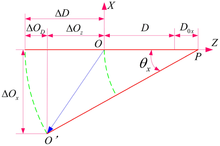
The geometric principle of the spindle thermal error compensation.
The compensation offset
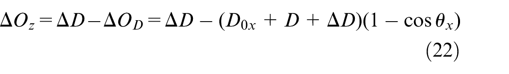
Because the axial elongation is far less than the length of the tool, that is

and
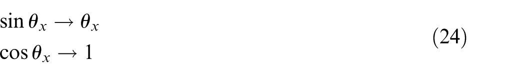
Substituting equations (23) and (24) into equations (21) and (22), thermal error compensation component in X- and Z-direction can be obtained, respectively


It can be seen that the X-directional compensation component is closely related to the tool length and that the offset in Z-direction has no relationship with the tool length. Similarly, the thermal error offset

where
Assuming that OW(Px, Py, Pz) is the coordinate of a point W on the workpiece before the thermal error compensation is conducted, the new coordinates of point W becomes

Namely
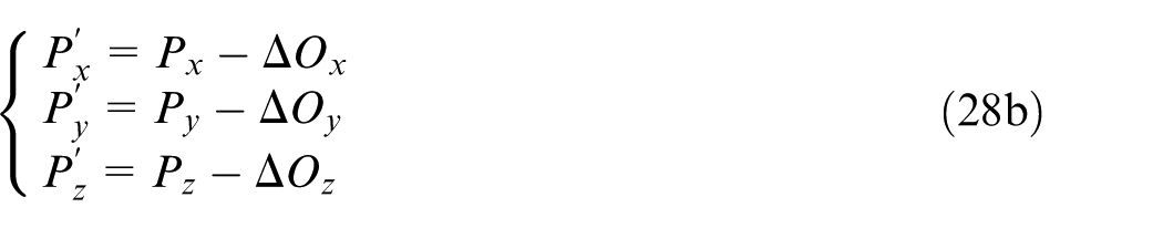
Substituting equations (25)–(27) into equation (28b)
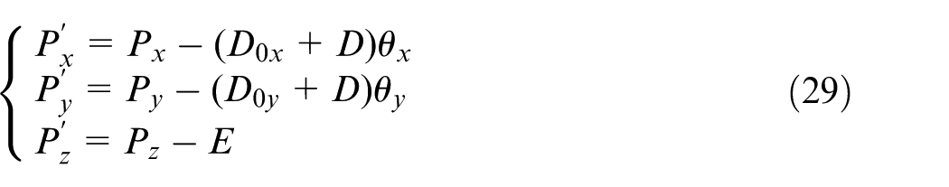
In the real-time online thermal error compensation process, the compensation component can be calculated according to the mathematical models of E,
Implementation of thermal error compensation
The thermal error compensation of high-speed system is conducted on a jig borer’s high-speed spindle to validate the effectiveness of thermal error modeling methods based on BP and GA-BP neural networks. And the temperature field and thermal errors of the spindle are measured by the temperature and eddy-current sensors mounting on the machine tool. And the values of the temperatures and thermal errors are sent to the procession module. And the thermal error models are established by the procession module. Thermal error compensation is conducted based on the compensation component computed by the procession module. And the compensation component is inserted into the machining instructions by the programmable logic controller (PLC).
Compensation results
The thermal error compensation of high-speed spindle system was conducted on a jig borer. The thermal error after compensation was measured and compared with the thermal error before compensation, as shown in Figure 7. And the parameters to evaluate the performance of the models based on BP and GA-BP neural networks were shown in Table 4.
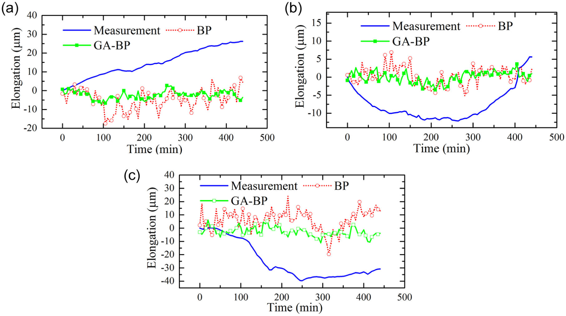
The compensation results comparison: (a) X-direction, (b) Y-direction and (c) Z-direction.
Compensation results.
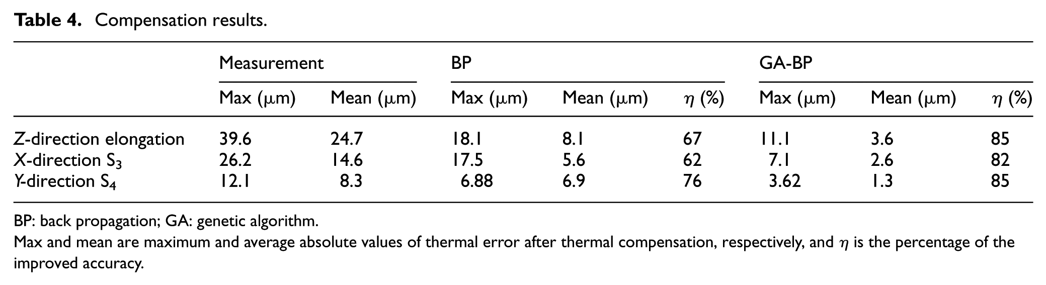
BP: back propagation; GA: genetic algorithm.
Max and mean are maximum and average absolute values of thermal error after thermal compensation, respectively, and
Table 4 indicates that the thermal error model based on GA-BP network performed perfectly than the BP network. After the compensation of thermal error, the error in the axial direction reduced significantly. For the GA-BP model, the axial maximum error is reduced from 39.6 µm to 11.1 µm, and the average error reduced from 24.7 µm to 3.6 µm. The axial accuracy is improved by 85%, which demonstrates the effectiveness of the proposed measuring, modeling and compensating methods, while the BP model could improve the accuracy only to 67%. The accuracy of radial thermal error S3 is improved to 82% by the GA-BP model. However, the accuracy of the X-direction can be only improved to 62%. Meanwhile, the accuracy of the Y-direction of the BP and GA-BP models is advanced by 76% and 85%, respectively.
Conclusion
In this article, to improve the accuracy, convergence and robustness of thermal error compensation models based on ANNs, two thermal error models were proposed based on BP and GA-BP neural networks, and the thermal errors of the high-speed spindle system were compensated to improve the machining accuracy of the jig borer effectively. Systematic thermal error measuring, modeling and compensating methods were proposed. And the following conclusions can be obtained:
Five eddy-current sensors were used to measure the thermal errors of the high-speed spindle. A novel method, which can be used to group temperature variables and select thermal sensitive points and exclude multicollinearity among temperature variables, was proposed so that the number of independent variables achieves minimum in thermal error models to improve the efficiency, stability and robustness of thermal error models. And the method of grouping temperature variables and selecting thermal sensitive points provided efficient theoretical guidance for the arrangement of temperature sensors instead of scholars’ engineering experience.
The modeling principle of the thermal error modeling method based on the traditional BP network was analyzed. Considering the shortages of traditional BP neural network which is simple and adaptive but converges slowly and is easy to fall into reach local minima, a GA was introduced to optimize the number of the nodes in the hidden layer, the initial weights and thresholds of the BP network. On the other hand, the method of thermal error modeling based on GA-BP neural network provides theoretical guidance for the determination the topology, the weights and thresholds of the BP network instead of the experience of researchers and repeated experiments. BP and GA-BP neural networks were trained with thermal error sampled data of high-speed spindle of a machine tool. The predictions of the GA-BP neural model showed that the accuracy, robustness and convergence were greatly improved compared with the traditional BP neural model.
Thermal error compensation equations of three directions were presented, considering thermal elongation and radial thermal tilt angles when thermal error compensation is conducted. Moreover, the thermal error compensation equations can accurately characterize the real position and pose when the spindle thermal deformation happened. And the thermal error compensation equations proposed in this article are effective and can improve the machining accuracy of machine tools by real-time compensation.
The thermal error compensation strategy was proposed. And a thermal error compensation module was developed based on the thermal error modeling method to realize real-time online thermal error compensation on Simens 840D.
The real-time compensation of the spindle thermal errors was conducted to validate the effectiveness of the BP and GA-BP models. The compensation results showed that the accuracy, robustness and convergence of the GA-BP neural model were much more excellent than the thermal error model based on traditional BP neural network and the GA-BP neural model was more suitable to be regarded the compensation model. And the thermal error model based on grey correlation analysis and traditional BP neural network has high fitting performance, and its prediction accuracy is above 94%. However, the predictive ability of the BP model is much lower than GA-BP model, and the convergence and generality are much worse than the GA-BP model. Therefore, the GA can be applied to optimize the number of the nodes in the hidden layer, the weights and thresholds of the traditional BP network.
By conducting real-time thermal error compensation, the machining accuracy of the machine tool was improved significantly. And the results showed that the axial machining accuracy of the jig borer was improved by 85%, the X/Y-direction accuracy was improved by 82% and 85%, respectively.
Footnotes
Declaration of conflicting interests
The author(s) declared no potential conflicts of interest with respect to the research, authorship and/or publication of this article.
Funding
This research is supported by the National High Technology Research and Development Program of China (Grant No. 2012AA040701).