
Abstract
The present error compensation technology of computer numerical control machine tools ignores radial thermal tilt angle errors of the spindle, while the thermal-induced offset is closely related to the tilt angle and the handle length. To solve this problem, three models of spindle thermal errors are proposed for the thermal yaw, pitch angles and elongation, and error compensation is performed based on the thermal tilt angles and cutting tool length. A five-point method was applied to measure the spindle thermal drifts at different speeds by eddy current sensors, which could effectively analyse the changes in the position-pose of the errors. Fuzzy clustering and correlation analysis were applied to group and optimise the temperature variables and select the variables sensitive to thermal errors in order to depress the multicollinearity of the temperature variables and improve the stability of the model. Finally, the thermal offset compensation was conducted in three directions. The results indicate that back propagation has a better capability for nonlinear fitting, but its generalisation is far less than that of time series. While the structure of multiple linear regression analysis is simple, its prediction accuracy is not satisfied. Time series adequately reflects the dynamic behaviours of the thermal error, and the prediction accuracy can reach 94%, with excellent robustness under different cutting conditions. The thermal error compensation equation that includes thermal tilt angles and cutting tool length is suitable for actual conditions and can accurately describe the space-pose of the thermal deformation and improve the machining accuracy.
Keywords
Introduction
Precision jig-boring machining has long been applied to manufacture complicated box-type parts. However, the accuracy may decrease and become far lower than the initial design value after the machine is used for a long period of time. This decreased accuracy over time primarily results from inadequate maintenance and accuracy stability and thermal error is the main factor leading to the inadequate accuracy, accounting for 70% of the total errors arising from various error sources. 1 Thermal error accounts for an increasing proportion of the total error as machining tools become more sophisticated. Moreover, the dynamical characteristics of the spindle also affect the thermal error. Zhang et al. 2 proposed a holospectrum-based balancing method to improve machining accuracy. Non-uniform temperature distribution causes thermal errors in computer numerical control (CNC) machine tools, and this distribution becomes nonlinear and non-stationary and varies with time. The mutual coupling of the location and intensity of the heat source, the thermal expansion coefficient and machine structure can create complex thermal characteristics. 3 Donmez et al. 4 proposed that changing temperatures produce thermal error, which is a major factor in the reduction in machining accuracy.
To study the thermal characteristics of a spindle, the temperature field and thermal errors must first be accurately measured. Existing measurement methods discussed in the literature mainly focus on the axial thermal elongation, while radial thermal tilt errors have not been sufficiently considered. In this article, five eddy current displacement sensors (five-point measurement) are applied to simultaneously measure axial and radial thermal deformations, and thermal error models are established based on the analysis of the space and pose of the thermal deformation.
There are two methods to establish the thermal error model, the theoretical model based on heat transfer and the experimental model. In recent years, the finite element method (FEM), which is used to analyse temperature fields and the thermal deformation of machine tools, has become a topic of particular interest. Min and Jiang 5 established a variety of thermal boundary conditions for a thermal error model based on the Fourier thermodynamic equation and analysed the temperature field distribution of the screw under different heat fluxes. Zhao et al. 6 proposed a method to calculate the thermal conductivity coefficient of the spindle surface and simulated and analysed the variation principles of the temperature field and the thermal deformation of the spindle. Creighton et al. 7 used the FEM to analyse the temperature distribution characteristics of a high-speed micro-milling spindle and constructed an exponential model of the axial thermal error related to the spindle speed and running time. However, the thermal error of a precision CNC machine tool is a mutual coupling of many complex factors that are affected by numerous variables; therefore, it is extremely difficult to establish a theoretical equation from the perspective of thermoelasticity and heat transfer.
When pure theoretic equations encounter difficulties, many scholars transfer their emphases to experimental research and construct thermal error models based on engineering experience. Neural networks can describe nonlinear mapping relationships very well. Since Rumelhart et al. 8 proposed learning methods of multilayer back propagation (BP), many scholars have begun to apply neural networks to thermal error modelling. Yang et al.9,10 used artificial neural networks (ANNs) to establish a relationship between the temperature and thermal error of a spindle, and the model proved to be useful for making generalisations. Ouafi et al. 10 constructed an ANN model for the spindle thermal error, with the temperature drawn based on a statistical methodology, and carried out error compensation experiments that effectively improved the machining accuracy. Multiple linear regression analysis (MLRA) with a simple structure is a traditional modelling method for the thermal error. Jenq and Wei 11 and Lee and Yang 12 established a compensation model for the spindle thermal error using an MLRA method. Hong and Ibaraki 13 studied the thermal characteristics of a rotary axis on the five-axis machine, analysed the effect of thermal error on errors in the motion of the rotary axis and calculated how errors in motion can be caused by thermal errors together with geometric errors. Vyroubal 14 presented a cost-effective method focused on the error compensation of the machine’s thermal deformation in the axis direction of the spindle based on decomposition analysis. Vissiere et al. 15 measured the thermal drifts of the spindle with a new method in which measurement accuracy can reach even the nanometre scale. Time series (TS) analysis provides a set of approaches to process the dynamic data. The essence of this method is that all types of data are approximately described by mathematical models. Through analysis of these models, the internal structure of the data can be analysed so that we can forecast its trends and apply necessary controls to it. Wang and Yang, 16 Miao et al. 17 and Wang et al. 18 applied the TS analysis method to establish a spindle thermal error model and used it to compensate for thermal errors, thereby obtaining better results. In this article, eddy current displacement sensors are used to measure spindle thermal errors; such sensors have the advantage of contact-free measurement. In recent years, new technologies have been used for the manufacture of such sensors. 19 PT100 has a high accuracy, and Frohlich et al. 20 quantitatively demonstrated its excellent stability, enabling it to be used for accurate temperature measurements.
With the thermal error model presented, the next work would be compensation for errors during machining. Fu et al. 21 and Miao et al. 22 built a model of the spindle axial thermal error using the multivariate linear regression method. Wang and Yang 16 also proposed a prediction model for the axial thermal deformation and applied the model to compensate a CNC machine. Ouafi et al. 10 presented a comprehensive modelling approach for real-time thermal error compensation based on multiple temperature measurements, and the thermal-induced errors of the spindle were reduced from 19 µm to less than 1 µm. There are other scholars who investigated the axial thermal error compensation method for the spindle, 23 and the machining accuracy was effectively improved. Zhang et al. 24 proposed a compensation implementation technique based on machine zero point shift and Ethernet data communication protocol for machine tools and thereby improved the machine accuracy.
Most of the present literature focuses on the axial expansion of the spindle, ignoring the radial tilt angle errors. However, thermal angle errors are key factors in compensating the terminal processing accuracy of the spindle. Thus, the spindle thermal error offset compensation should also consider the tilt angles and the length of the cutting tool. Therefore, in this article, three methods are proposed to modelling the spindle thermal errors on a jig-boring machine, considering the radial yaw and pitch angles and the length of the cutting tool, and the criteria for estimating the prediction goodness of the models are established. Thermal balance experiments were performed using a temperature displacement acquisition system to synchronously measure the temperature distribution and thermal deformation at different spindle speeds, and the effects of different spindle speeds on thermal characteristics were analysed. The fuzzy clustering analysis method was used to optimise the temperature variables, selecting the variables that were thermal error–sensitive. multi-input and multi-output (MIMO) ANN, MLRA and TS models were proposed for the axial elongation and radial thermal tilt angles of the spindle. Subsequently, a new set of sample data was used to validate the model robustness, and the predictive goodness of the three models was compared. Finally, the thermal offset compensation based on the cutting tool length and thermal tilt angles was conducted in three directions on the CNC machine, and the three models’ compensative efficiencies were analysed.
Experimental principles and equipment
Experimental system
The experimental system is shown in Figure 1, which focuses on the spindle of a precision CNC jig-boring machine. The changes in the temperature field and the thermal distortion of the spindle can be analysed by this system. The maximum speed of the spindle is N = 20000 r/min, and the cooling system of the spindle is controlled intelligently by the temperature. The front and rear bearings and motor are cooled.
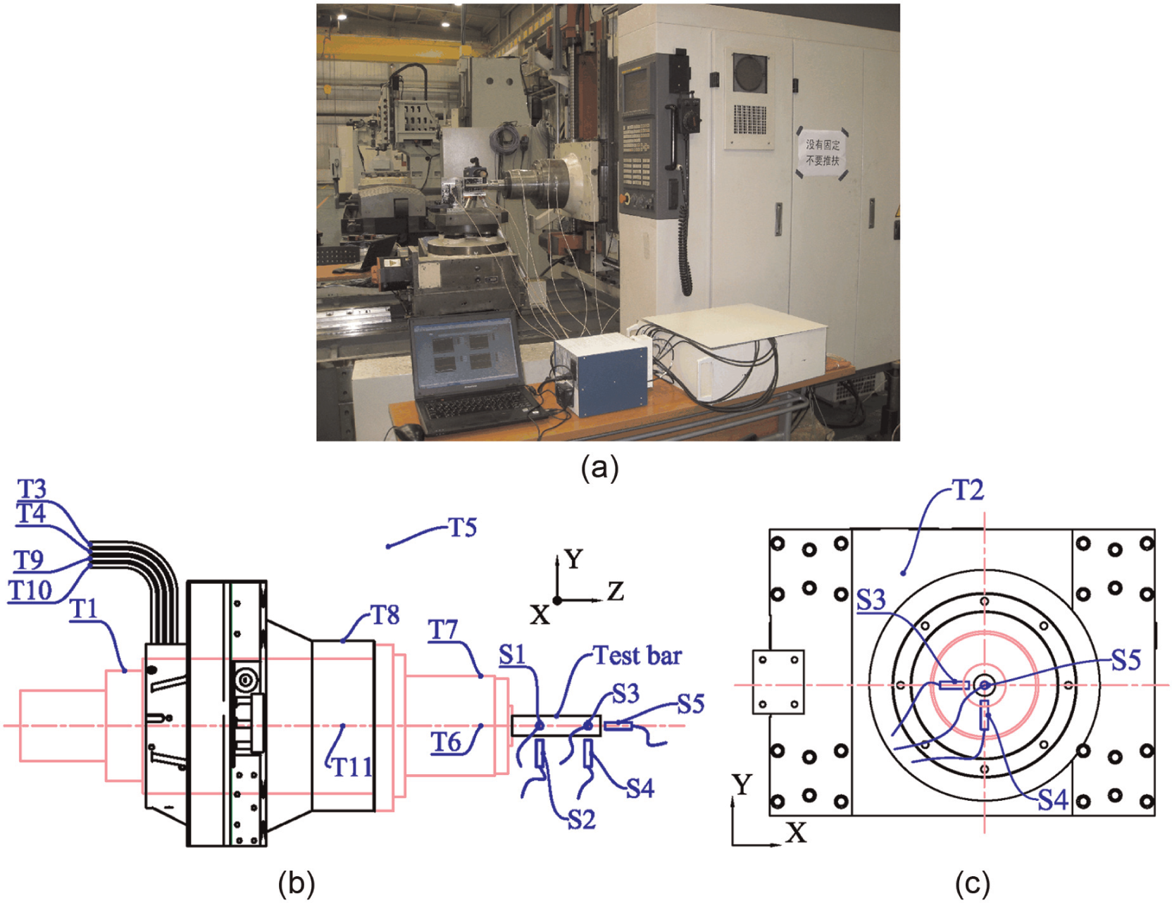
Spindle experiment setup: (a) boring machine and measurement system, (b) left view and (c) front view.
The measured equipment and functions are as follows: a synchronous acquisition system (developed by our group based on NI SCXI) is used to determine the temperatures and the thermal deformations. This system uses the precise magnetic temperature sensors of the Pt100 to measure the temperatures of the motor, bearings, pedestal and coolant of the spindle system and environment. High-precision eddy current sensors are utilised to measure the spindle thermal drifts. The system performs real-time synchronous acquisition of temperatures and thermal drifts.
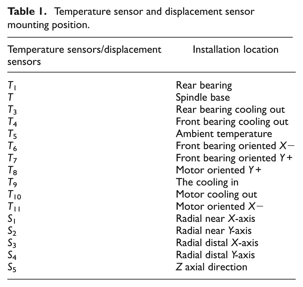
Table 1 presents and describes the positions of the sensors on the machine. Temperatures are denoted as T 1,…, T 11, and the eddy current displacement sensors are defined as S 1,…, S 5.
Temperature sensor and displacement sensor mounting position.
Measurement principle
The spindle thermal drifts are measured by a five-point method,
25
with the displacement sensor fixture and measurement diagram shown in Figure 2. The spindle is parallel to the Z-axis, and the axial thermal expansion can be obtained by S
5. The radial thermal yaw
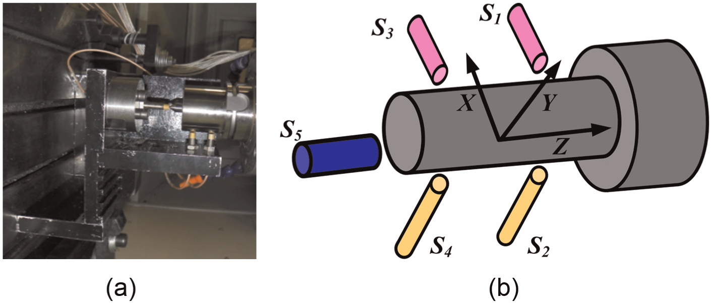
Spindle five-spot installation diagram: (a) the sensor fixture and (b) five-point measurement sketch map.
After the spindle has run for a long period, thermal elongation expands the axial direction, and thermal angle change causes a tilt in the radial direction due to the uneven gradient distribution of the temperatures, as shown in Figure 3, where the thermal yaw angle

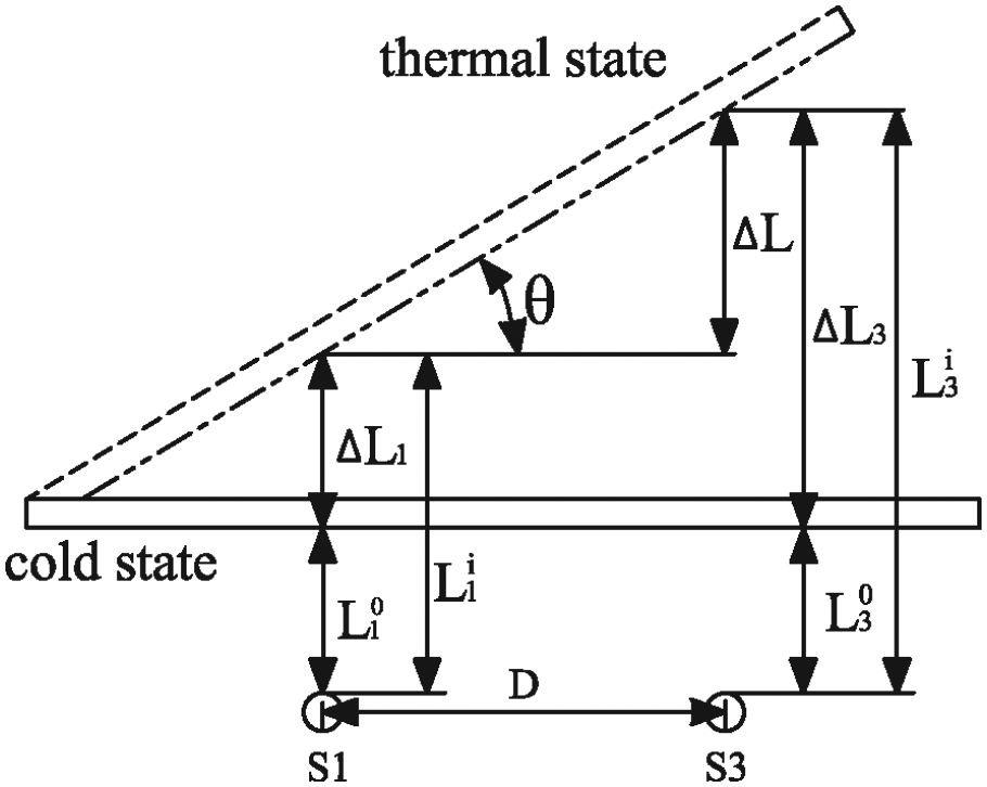
Spindle thermal inclination sketch.
where i denotes the number of measurements. The thermal yaw angle is too small in this experiment (i.e.

The thermal yaw can be obtained by applying equations (1) and (2)

where
Similarly, the thermal pitch angle

Experimental results and analysis
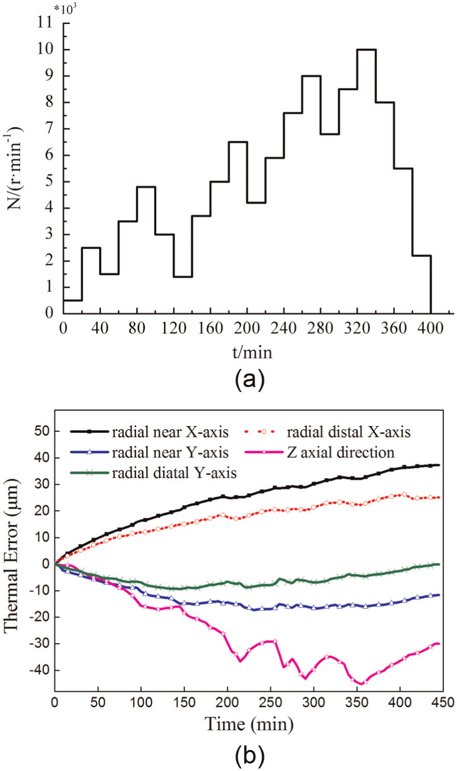
The spindle speed affects the distribution of the temperature field and the magnitude of the thermal drifts. This section focuses on a set of experimental data. To simulate the actual changes in the spindle speeds during processing, the velocity was varied in the experiment, as shown in Figure 4.
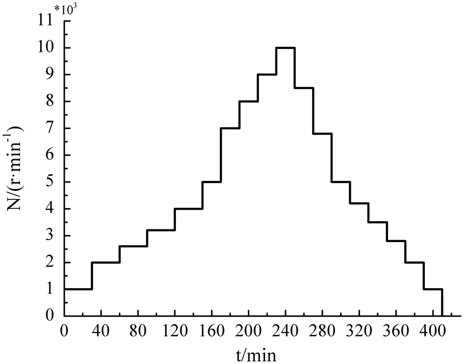
Distribution of the step speeds.
Time-domain analysis of thermal errors
The thermal drifts of the spindle are shown in Figure 5. The measurements indicate that the displacement trends increased gradually over time, eventually reaching thermal equilibrium. The axial elongation increased over time, and the direction was negative, which indicates that the elongation of the spindle expanded in the negative direction on the Z-axis. The time to equilibrium was approximately 385 min, with a maximum elongation of 39.6 µm. The thermal error was positive in the X-axis direction, which indicates that the spindle moved away from displacement sensors S
1 and S
3 during operation, deviating from the Z-axis and swinging to the negative direction of the X-axis on the XZ plane. The thermal yaw angle with the Z-axis is
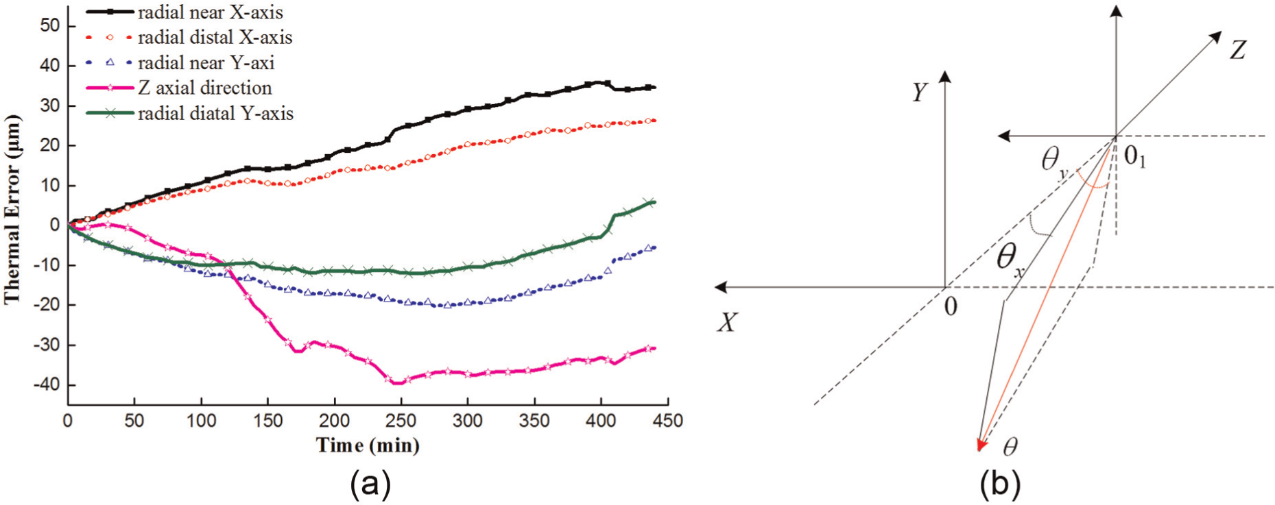
Thermal drifts of the spindle: (a) thermal errors and (b) the position and pose of the thermal spindle.
Temperature field distribution
The temperature variations in the spindle system are shown in Figure 6. The temperature trends of all measured points increased with time, but the increasing curves of the temperatures exhibited cyclical changes because the temperatures of the spindle were controlled by an intelligent cooling system, which set a threshold to reduce the temperature. If the temperature of the components reached this threshold, the cooling system activated. Therefore, the temperature exhibited fluctuation changes.
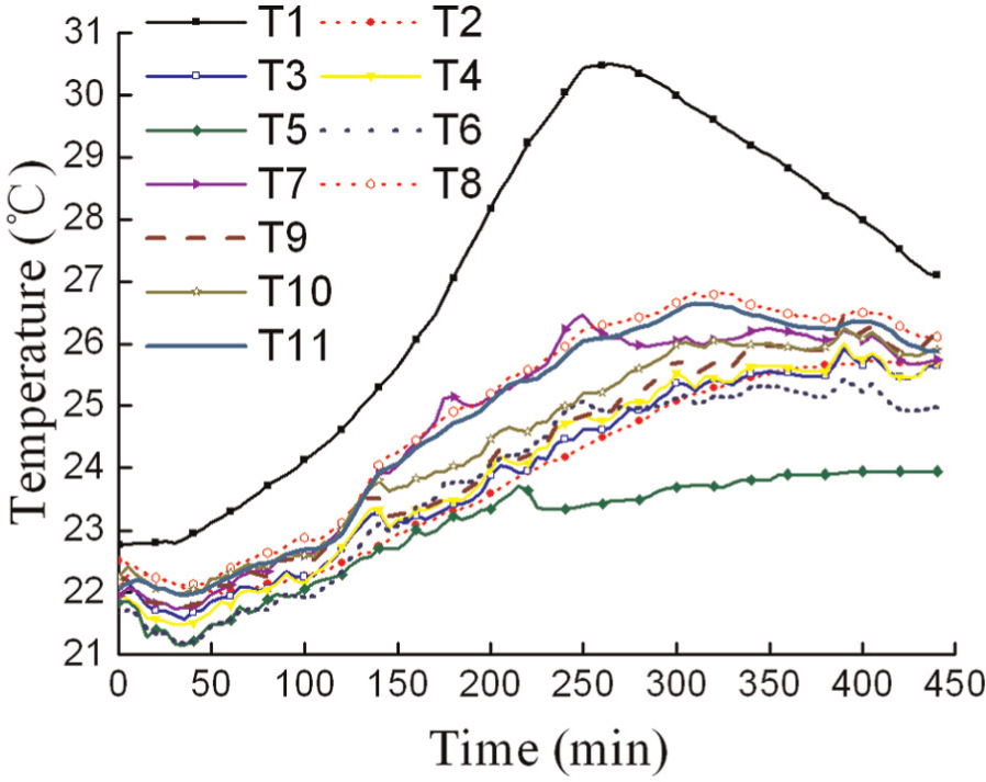
Temperatures of the spindle.
As the front bearing, rear bearing and the motor were cooled separately, temperatures could be inhibited from unbounded increase. However, the heat removed by the cooling fluid was less than the heat generated by the spindle, so the overall trend was still an increase to thermal equilibrium. Approximately 320 min was required for the temperature to reach thermal equilibrium, at which point the rear bearing had the highest temperature of 30.4 °C due to its large capacity, heavy load and severe friction, which generated more heat. The motor temperature was 26.7 °C. The temperatures of the other measured points were approximately 26 °C.
Temperature fuzzy cluster grouping and optimisation
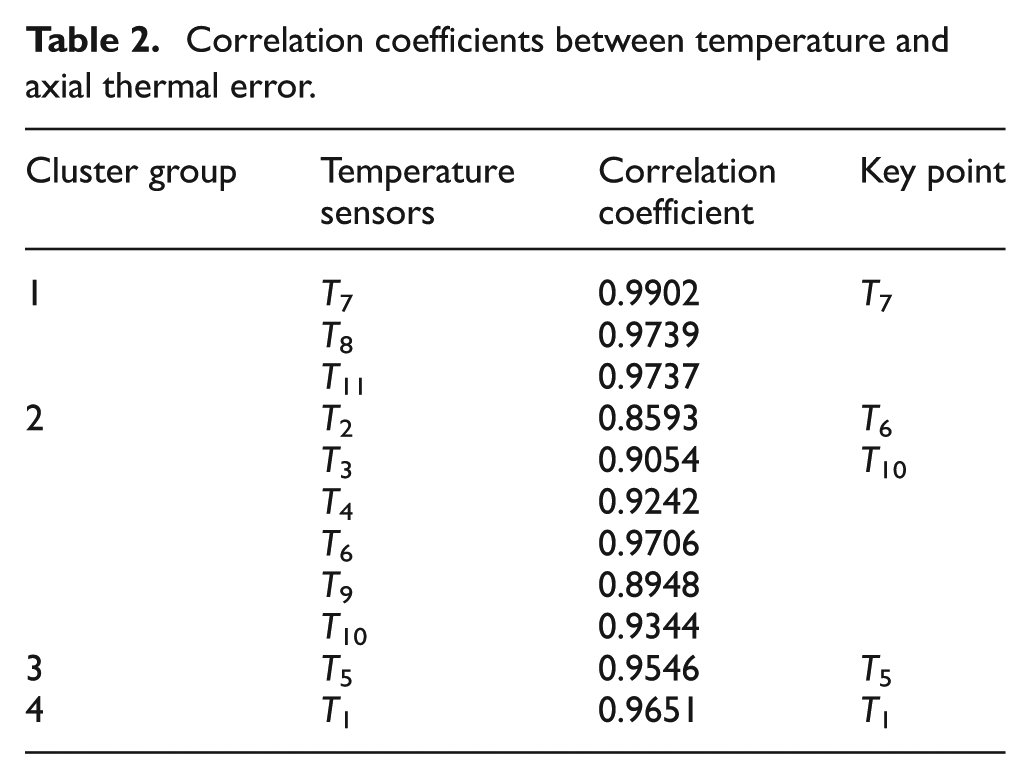
The famous scholar Ruspini 26 was the first to propose the concept of fuzzy partition. Specifically, Ruspini introduced fuzzy set theory into cluster analysis. Other researchers then presented a variety of the fuzzy clustering analysis method based on fuzzy graph theory, including the biggest tree method based on fuzzy graph theory. 27 This article groups the temperature variables of 11 measuring points using fuzzy clustering, applies statistical correlation to optimise the measuring points and calculates the correlation coefficient between each temperature variable and thermal error. Finally, the measurement points with the greatest correlation coefficients in each group are taken as the typical temperature variables.
Temperature fuzzy clustering
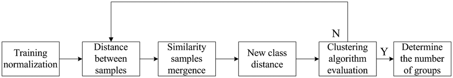
As the temperature variables have small values, system cluster analysis was used, and the variable packet flow is shown in Figure 7.
Fuzzy clustering grouping.
Assuming the temperature variable T = {T
1, T
2,…, Tm
} is the object to be analysed by fuzzy clustering, each object in T is Tk
(k = 1, 2,…, m), whose characteristics can be described by a limited number of values. Therefore, there is a corresponding vector P(Tk
) = (Tk
1, Tk
2,…, Tks
) matched with the object Tk. Tkj
(j = 1,2,…, s) is the jth characteristic value of Tk. P(Tk
) is the set of eigenvectors for Tk
. The sample T is divided into c fuzzy subsets
Cluster analysis is also known as the hierarchical clustering method. The feature vectors are gradually clustered according to the distance criteria. The classification moves from greater to lesser distance until it reaches the desired classification. The general steps of system clustering are as follows:
Initialise the data. Assuming that the sample set T contains m subsets T
1
(0), T
2
(0),…, Tm
(0), which form one class, calculate the distance between each pair of subsets and obtain a distance matrix
Find the smallest element in the distance matrix
Compute distances between the new categories to obtain the distance matrix
Repeat the second step until the classification meets the requirements.
For m = 11, the number of packets is set to C = 4. After calculating, the optimal grouping is obtained using the clustering algorithm of the combination of Euclidean-centroid, as shown in Figure 8. The temperature variables are divided into Groups {T 1}, {T 5}, {T 2, T 3, T 4, T 6, T 9, T 10}, {T 7, T 8, T 11}.
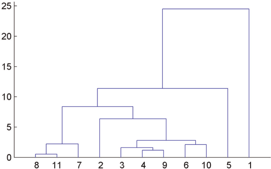
Clustering dendrogram.
Optimisation of temperature variables
Based on the results of the above groups, correlation coefficients between the axial thermal error E and the temperature Ti can be calculated
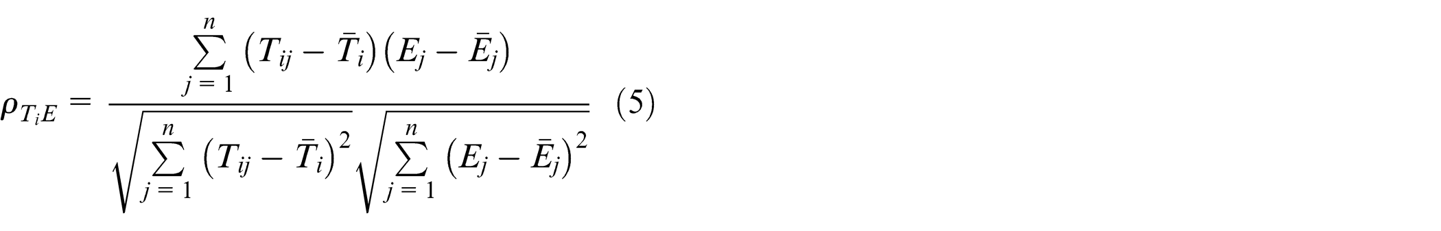
In the equation above, i = 1, 2,…, m is the ith measurement point of the temperatures, and j = 1, 2,…, n is the number of measurements. Tij
is the temperature of the ith measured point at the jth measurement. Ej
is the thermal elongation at the jth measurement,
Correlation coefficients between temperature and axial thermal error.
Thermal error modelling and prediction
Based on the five typical temperature variables determined by the packet optimisation, three spindle thermal error models are established, and the performance of the models is estimated through criteria provided to evaluate the goodness of the fitting.
Linear regression analysis
Linear regression analysis is a valid statistical method of determining an interdependent quantitative relationship between two or more variables. According to the principle of minimum error, a mathematical model describing the statistical relationship of the variables is determined.
MLRA
Assuming that there is a linear relationship between the dependent variable y and independent variable

where
For n sets of experimental data
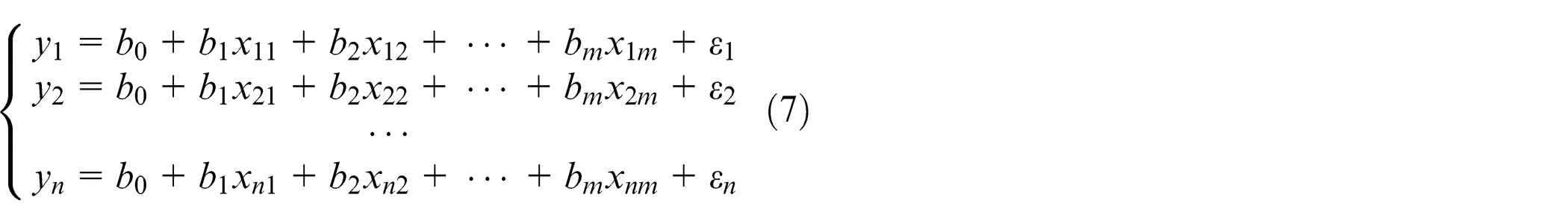
Then, presume
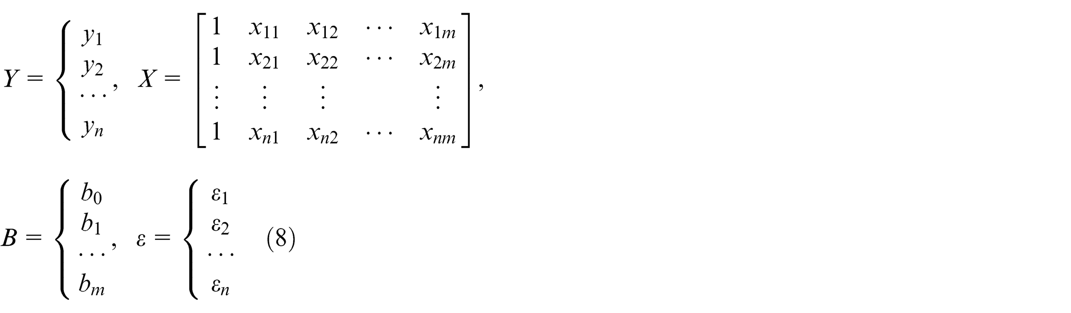
Equation (7) becomes

Equation (9) is a matrix form of the MLRA model.
Least-square estimation of parameters
Assuming that parameters

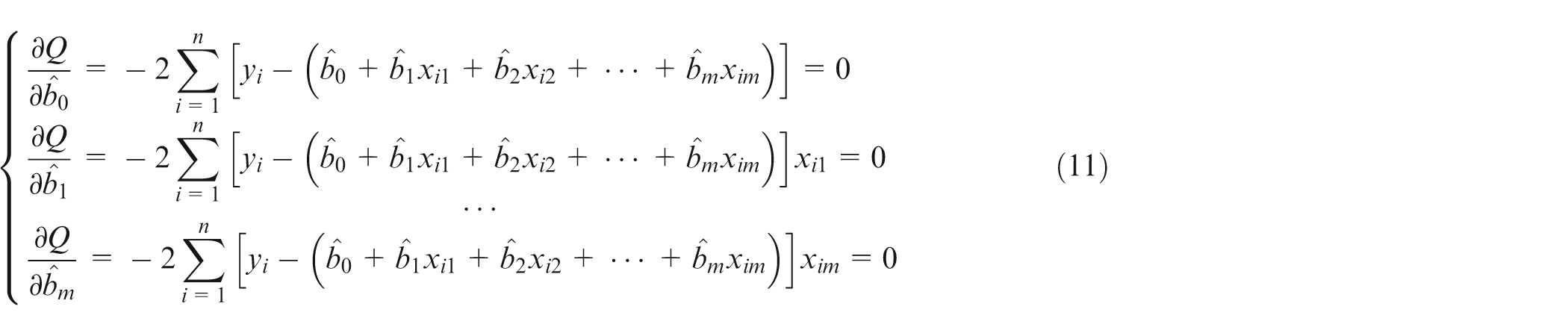
That is
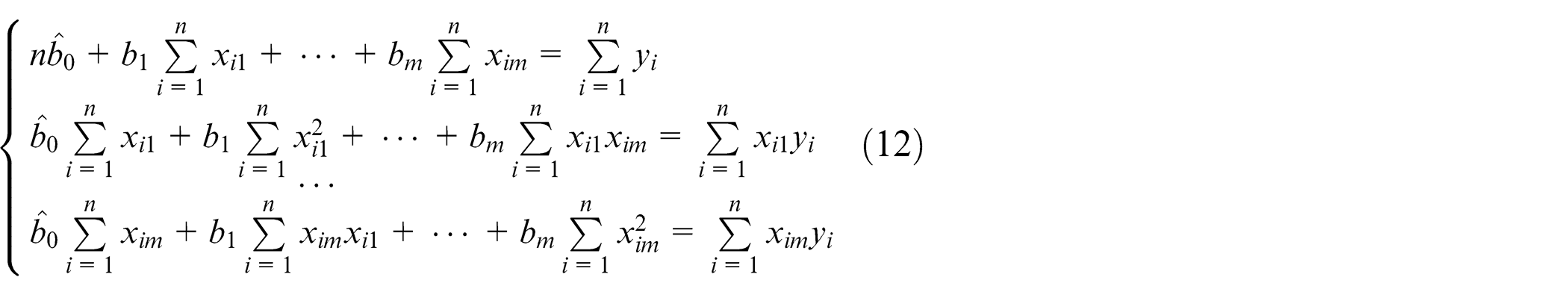
Equation (12) can be written in the form of a matrix formula

If the matrix
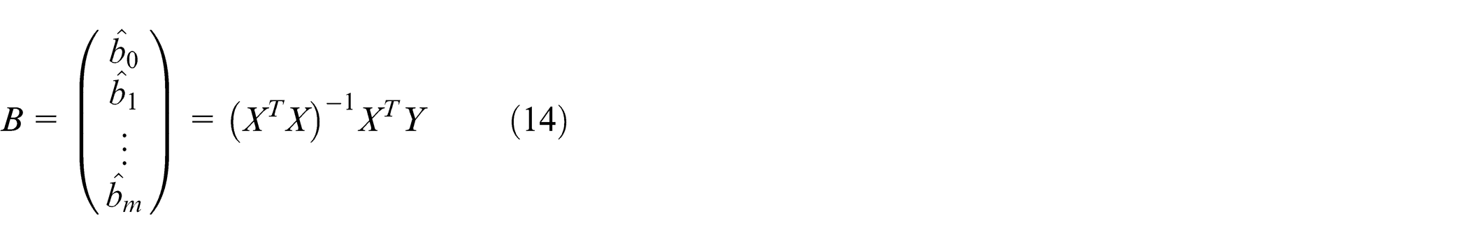
Vector B is the least-square estimation of the MLRA model.
The maximum coefficient R 2 is applied to determine a combination of independent variables
The identified temperature variables
MIMO neural network modelling
BP model
The relationship of the spindle thermal error to temperature is strongly nonlinear. An MIMO model of the thermal error is established based on a feedback neural network (BP)

where
Model structure
Setting a desired target, the efficiency of learning and the number of the iteration, the network is trained using the trainlm algorithm. Figure 9 illustrates the structure of the model: the hidden layer contains two layers made up of 5 × 1 neurons. The network constitutes five temperature variable inputs and three thermal drift variable outputs.
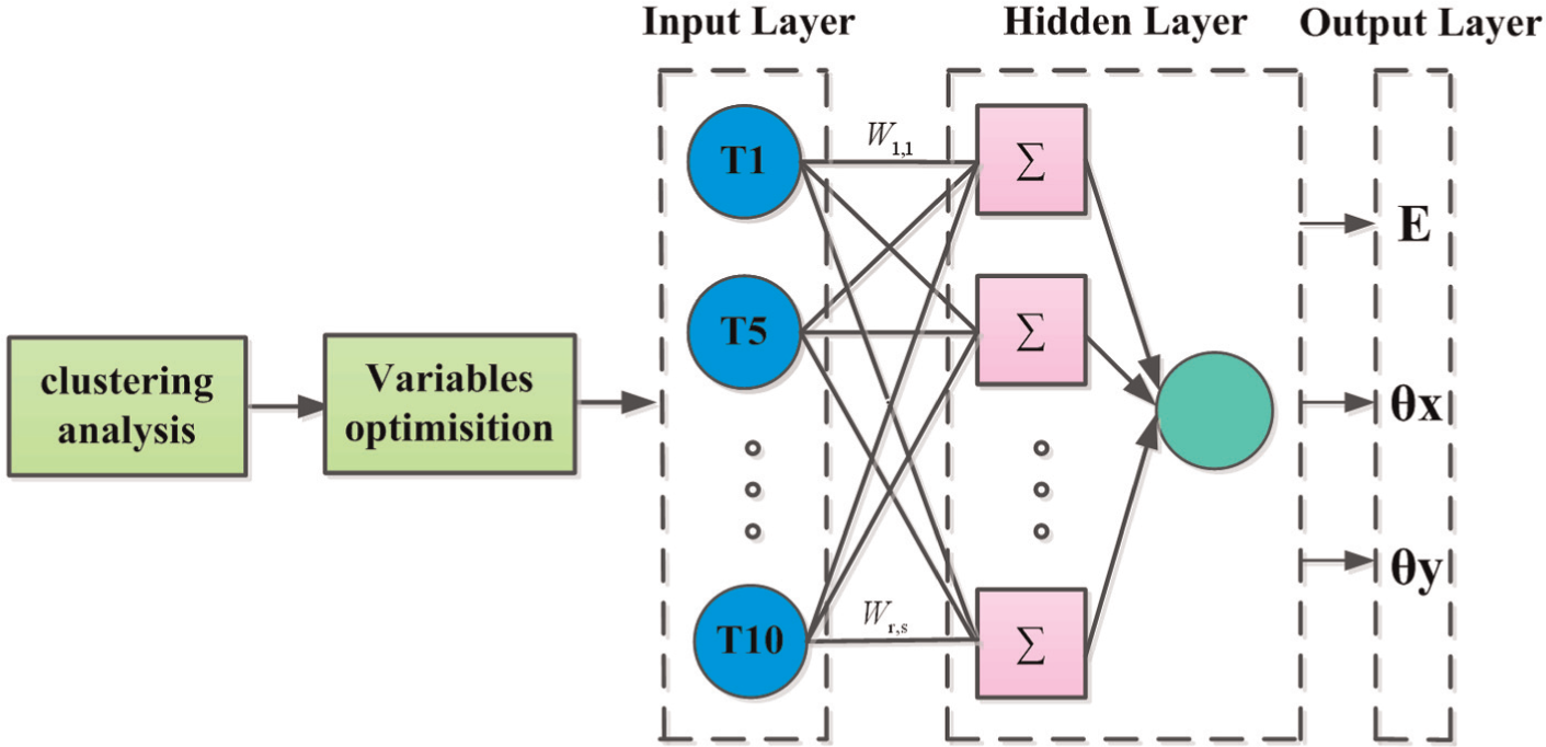
Neural network structure.
TS analysis
The basic idea of the TS analysis is that a mathematical model is established through the analysis of the time sequence of samples based on limited data of the observation system, accurately reflecting the dynamic dependency of the system, which is applied to predict and monitor the future behaviour of the system.
Stationarity determination and standardisation of thermal error sequence
Given that the sequence


where
The original sequences of the spindle thermal errors undergo standardising processing
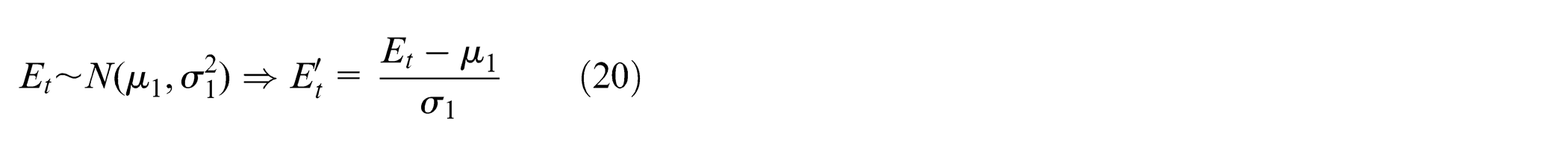


where
Model identification and parameter estimation
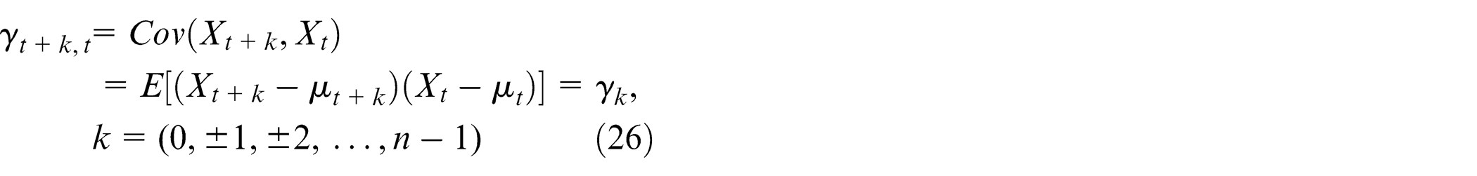
The autocorrelation function (ACF) and the partial autocorrelation function (PACF) are applied to calculate the tailing of the series, and the results indicate that the new TS of the standardised thermal errors are the autoregressive and moving average hybrid model autoregressive moving average (ARMA)(p, q), which is as follows 29

where

the ARMA model is transformed into

Box et al. 29 suggested that if the ARMA(p, q) model contains p order autoregressive AR(p) and q order moving average MA (q), its ACF is a pattern mixed exponential and attenuation sine wave after p-q order delay. Correspondingly, the partial correlation function is not an exact exponential form but, rather, is controlled by a mixture of index and decaying sine wave. The covariance is
The ACF is

According to statistical theory, the covariance function of TS with stationarity and 9 mean is estimated as follows

Thus, the ACF is estimated as follows
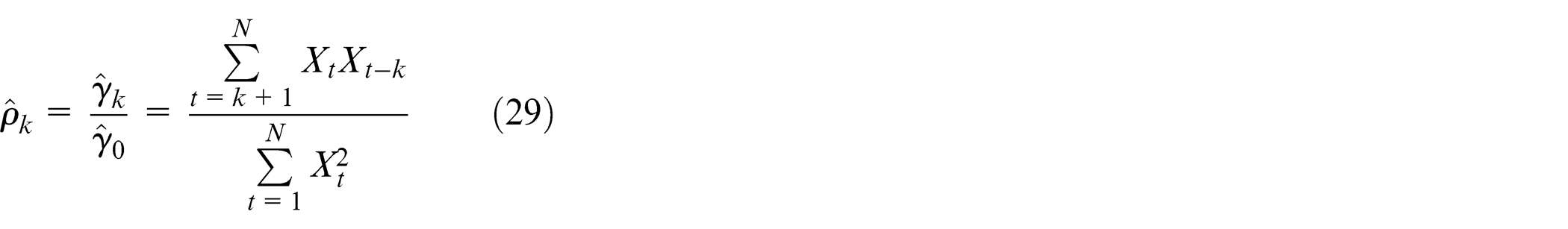
Yule–Walker equations can obtain autoregression coefficients; set
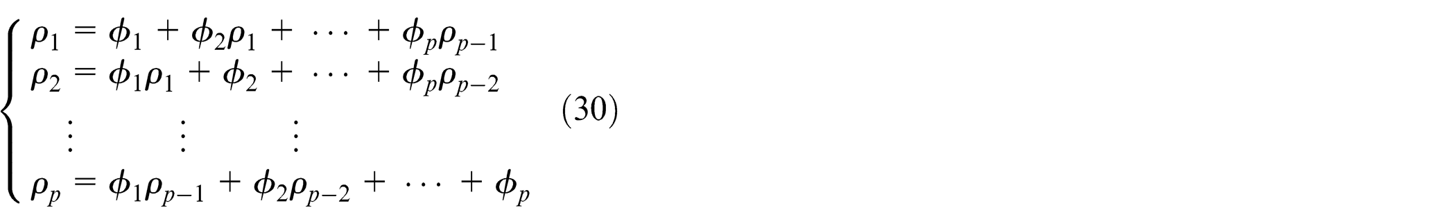
Replacing the theoretical autocorrelation
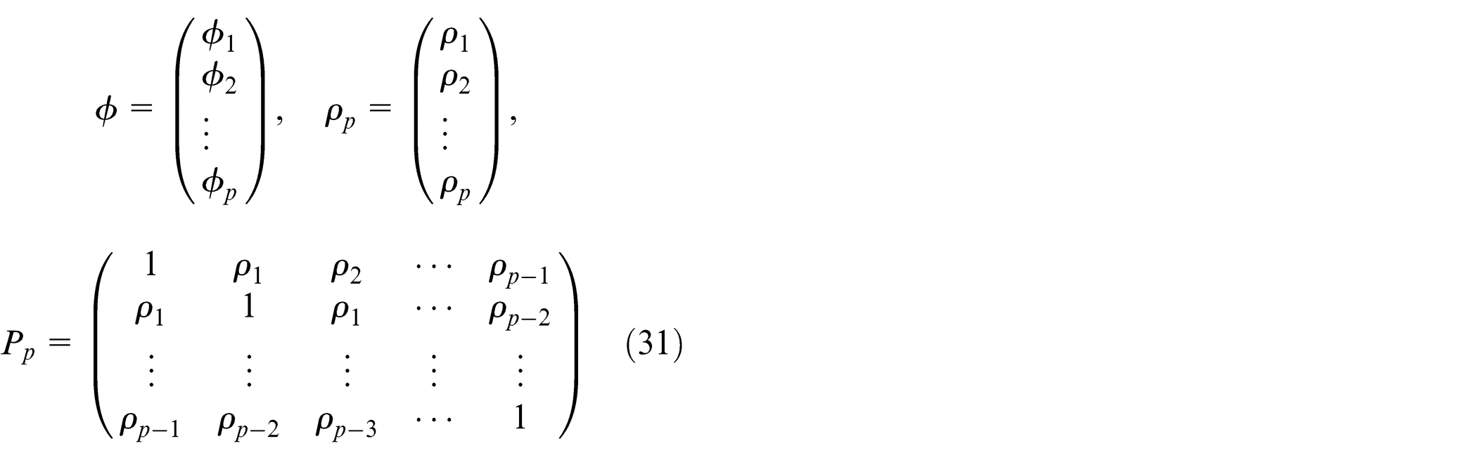
the parameter

Defining

the covariance
Using the convention that


Estimations of the parameters


Setting the order range

where
After calculation, the new TS
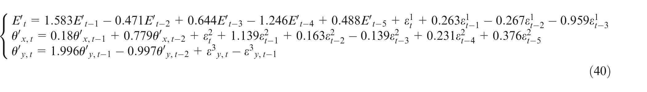
Assuming that vector
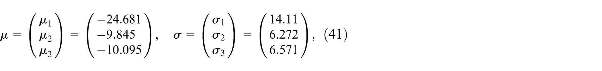
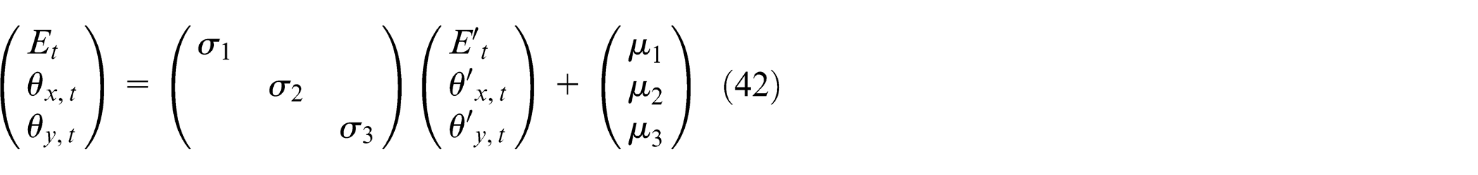
the new TS are reversed according to the following transformation, and the final spindle system thermal error model is
Model predictions and comparison
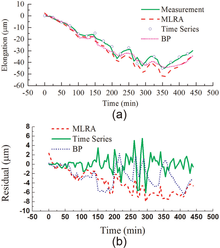
The experimental data in Figure 4 are taken as the training sample, and the sample data number is 89. Then, the three models – MIMO neural network (BP), MLRA and TS – are used to predict the thermal drifts of the spindle. The predicted and the measured values are compared in Figures 10–12.
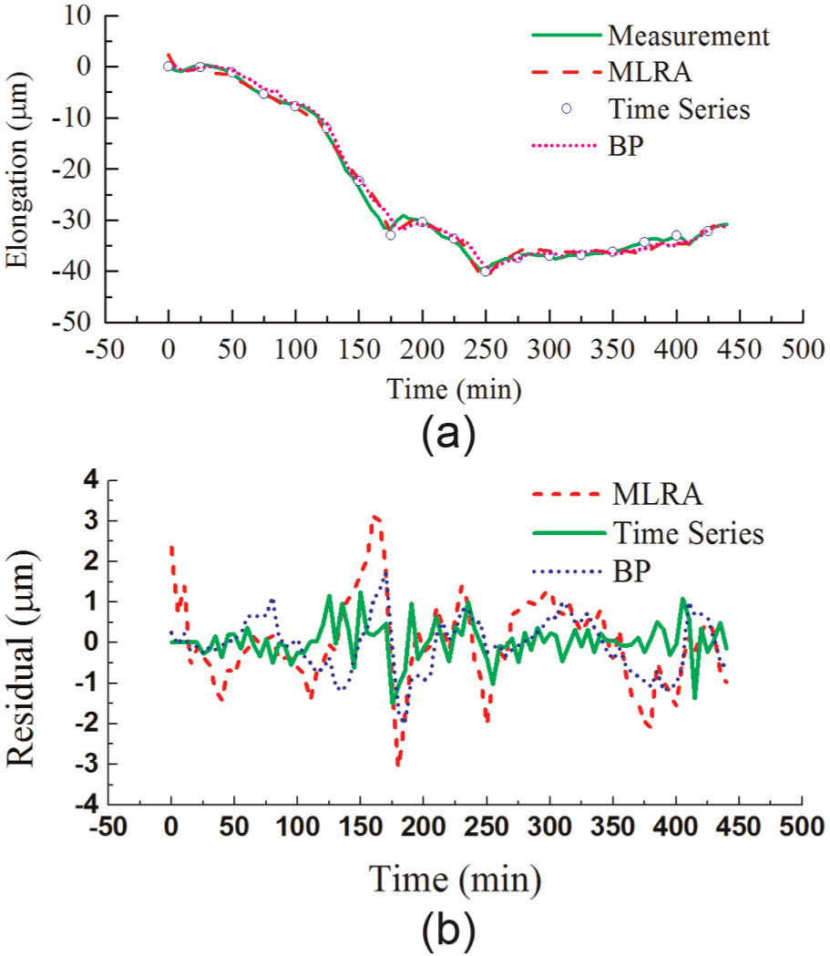
Axial thermal elongation: (a) prediction and measurement and (b) residual error.
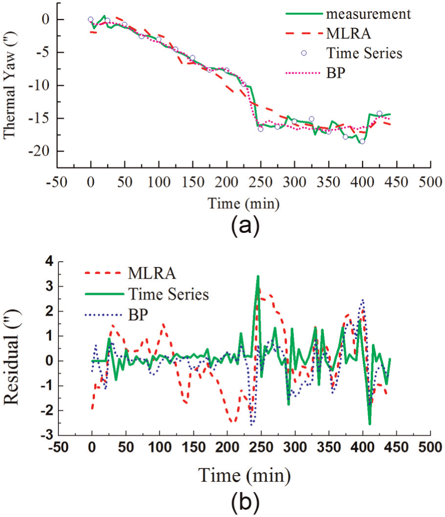
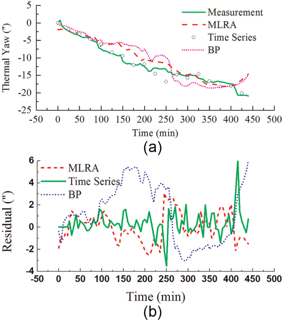
Radial thermal yaw angle error: (a) prediction and measurement and (b) residual error.
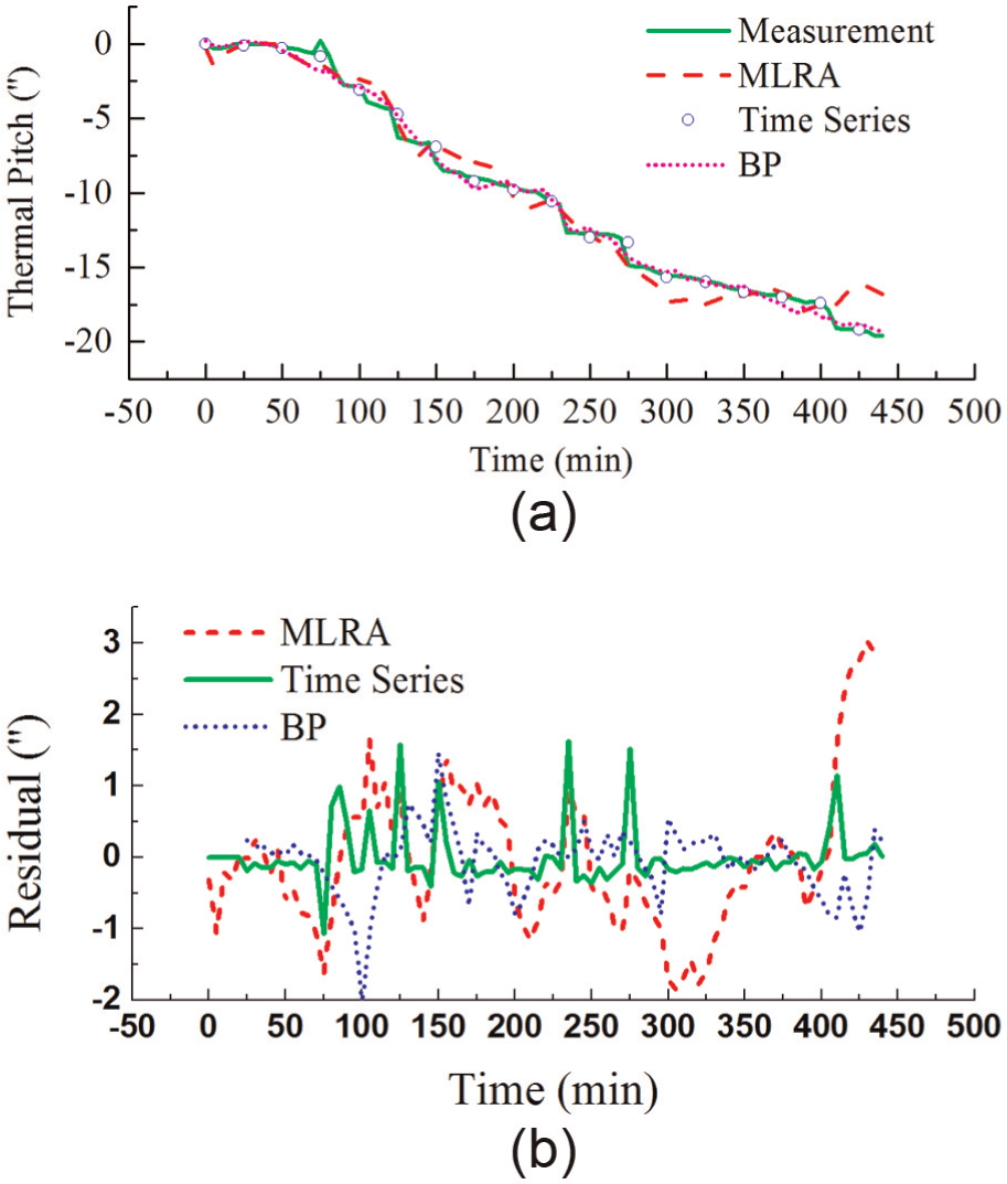
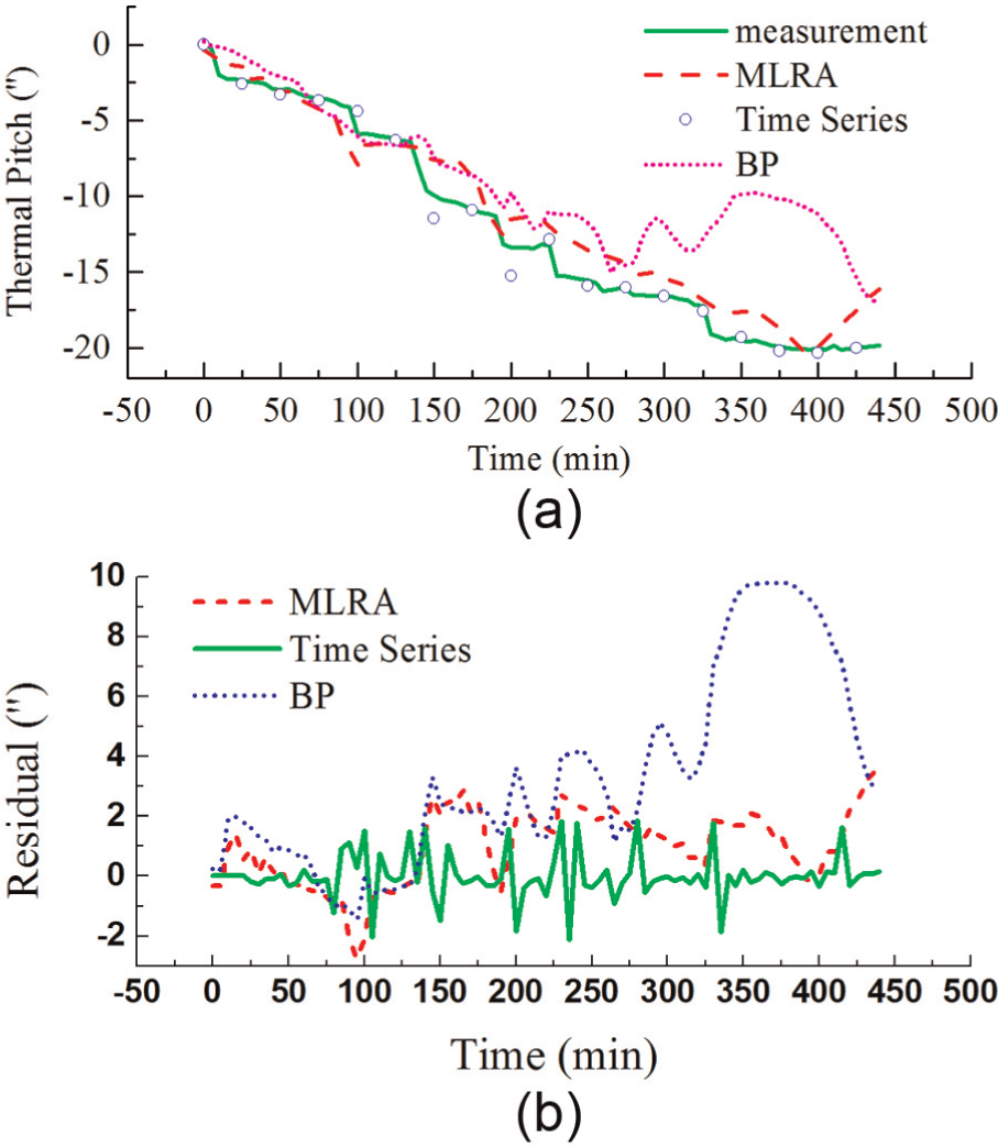
Radial thermal pitch angle error: (a) prediction and measurement and (b) residual error.
Next, we establish the evaluation criteria for the model fitting. Assuming the absolute value of the residual error is

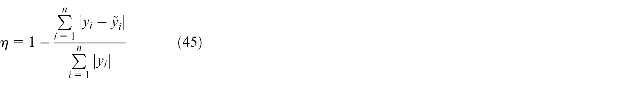
where
Fitting goodness parameters for thermal elongation E.
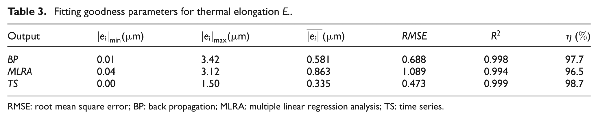
RMSE: root mean square error; BP: back propagation; MLRA: multiple linear regression analysis; TS: time series.
Fitting goodness parameters for thermal yaw angle
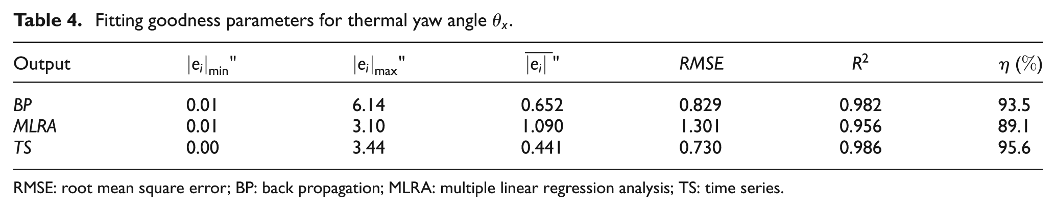
RMSE: root mean square error; BP: back propagation; MLRA: multiple linear regression analysis; TS: time series.
Fitting goodness parameters for thermal pitch angle
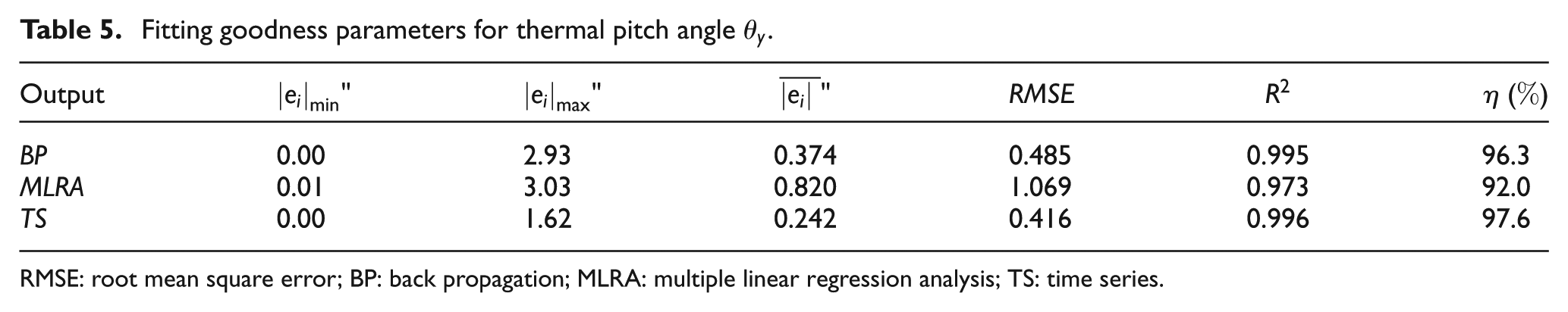
RMSE: root mean square error; BP: back propagation; MLRA: multiple linear regression analysis; TS: time series.
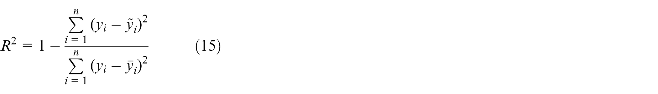
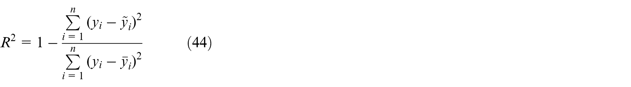
The determination coefficient R 2 can then be calculated with a boundary region of [0, 1], which characterises the extent to which the original data fall within the curve at a certain confidence level, with a larger R 2 indicating that the curve fits the original data better, and that the argument for explaining the model is more powerful. The root mean squared error of the fitted and measured values is denoted by RMSE, which indicates how closely the curve fits the original measurement data; a smaller value (closer to 0) indicates that the original data are more concentrated around the fitted curve on both sides. Analysing the parameters of fitting goodness in the three tables shows that the prediction behaviour of the three models is very good, and the maximum residual error, minimum error and average absolute error are very small, which indicates that the accuracy of the three models is high. The RMSE is near 0, and the determination coefficients are also close to 1. The prediction accuracy can reach 90%, and it further exhibits a strong fitting ability. The TS model is better than the BP neural network, which is superior to the MLRA.
Model validation
To verify the universality and generalisation of the models, a new data sample is used to predict the spindle thermal errors. Figure 13 describes the spindle speeds map and experimental results.
New air cutting condition: (a) random distribution of the speed and (b) thermal drifts.
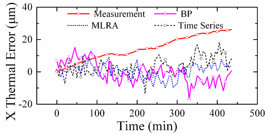
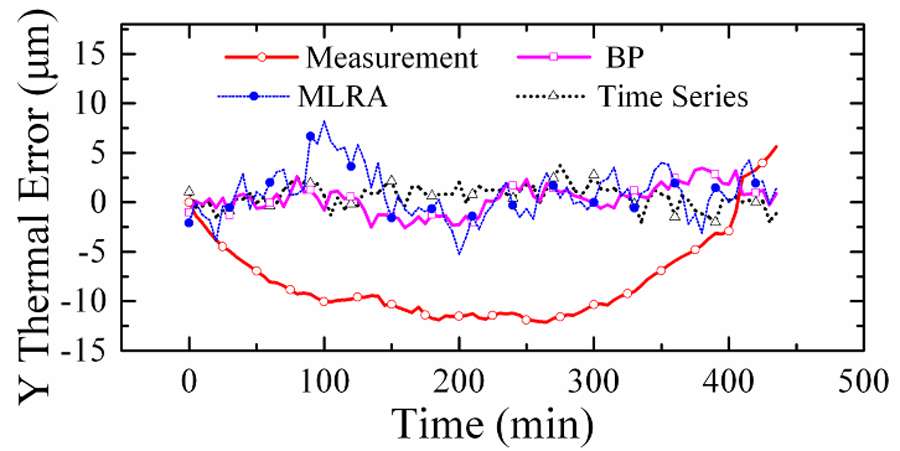
Then, using the BP, MLRA and TS models to predict thermal errors in the three directions of the spindle, the predicted values are compared to the measurements, as shown in Figures 14–16.
Axial thermal elongation: (a) prediction and measurement and (b) residual error.
Radial thermal yaw angle error: (a) prediction and measurement and (b) residual error.
Radial thermal pitch angle error: (a) prediction and measurement and (b) residual error.
The prediction-goodness parameters of the three models are presented in Tables 6–8. For E,
Prediction-goodness parameters for thermal elongation E.
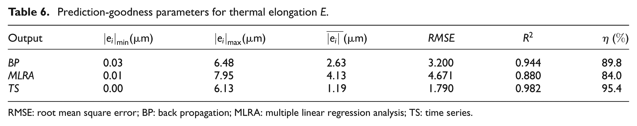
RMSE: root mean square error; BP: back propagation; MLRA: multiple linear regression analysis; TS: time series.
Prediction-goodness parameters for thermal yaw angle
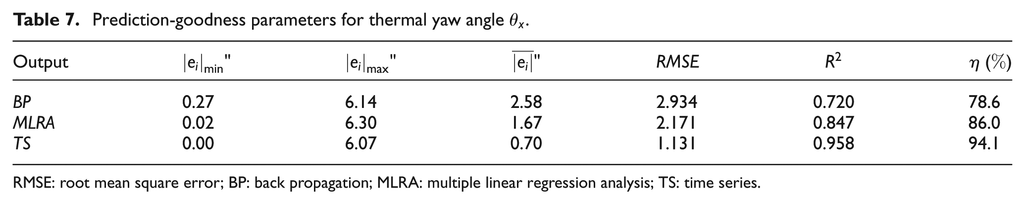
RMSE: root mean square error; BP: back propagation; MLRA: multiple linear regression analysis; TS: time series.
Prediction-goodness parameters for thermal pitch angle
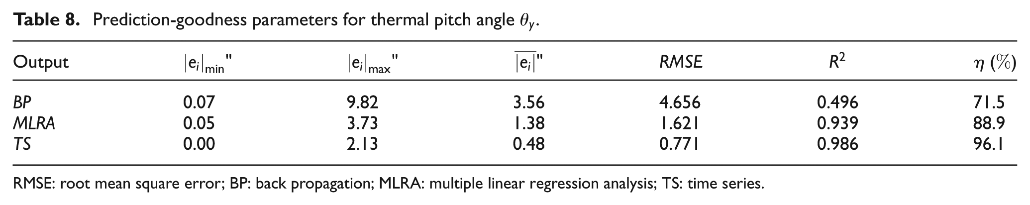
RMSE: root mean square error; BP: back propagation; MLRA: multiple linear regression analysis; TS: time series.
Comparison of the prediction-goodness parameters of the three models shows that when the spindle speed condition changes, the predictive abilities of all models for new data decrease. However, the forecasting accuracy of the TS model remains above 90%, indicating that TS can adequately reflect the dynamic characteristics of spindle thermal errors, and it provides excellent generalisation under different conditions. In contrast, BP has a powerful fitting capability and can perfectly describe the nonlinear relationship of temperatures with spindle thermal errors, but the model is strongly dependent on the training sample. Under new conditions, its prediction-goodness parameters drop sharply, even becoming far lower than the traditional MLRA model.
Model universality analysis
We now further explain the robustness of the TS model for application to different cutting conditions and its capability to adequately reflect the thermal error dynamic characteristics.
1. The temperature rate of the spindle system has a great influence on the thermal error, affecting the model prediction accuracy.
The essential reason for thermal errors is the existence of a temperature gradient in the spindle system. The uneven distribution of the temperature field of the spindle causes different thermal expansions of the components, which causes a relative deviation of the geometric positions among the parts, leading to thermal deformation. The influence factors of the spindle thermal characteristics are very complex, as the rotor and stator of the motor, bearings and other components can generate different amounts of heat per unit time in different operating conditions so that the temperature rate
In the two groups of experiments with different speeds, even if the temperatures are the same, the corresponding thermal deformations are not entirely equivalent, as shown by a comparison between the working condition for training models (1) shown in Figure 4 and the working condition for the validation of the models (2) shown in Figure 13(b). Figures 17–19 show that E,
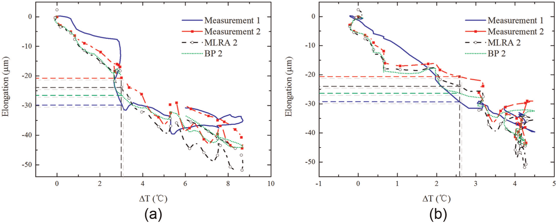
Axial thermal elongation with temperature: (a)
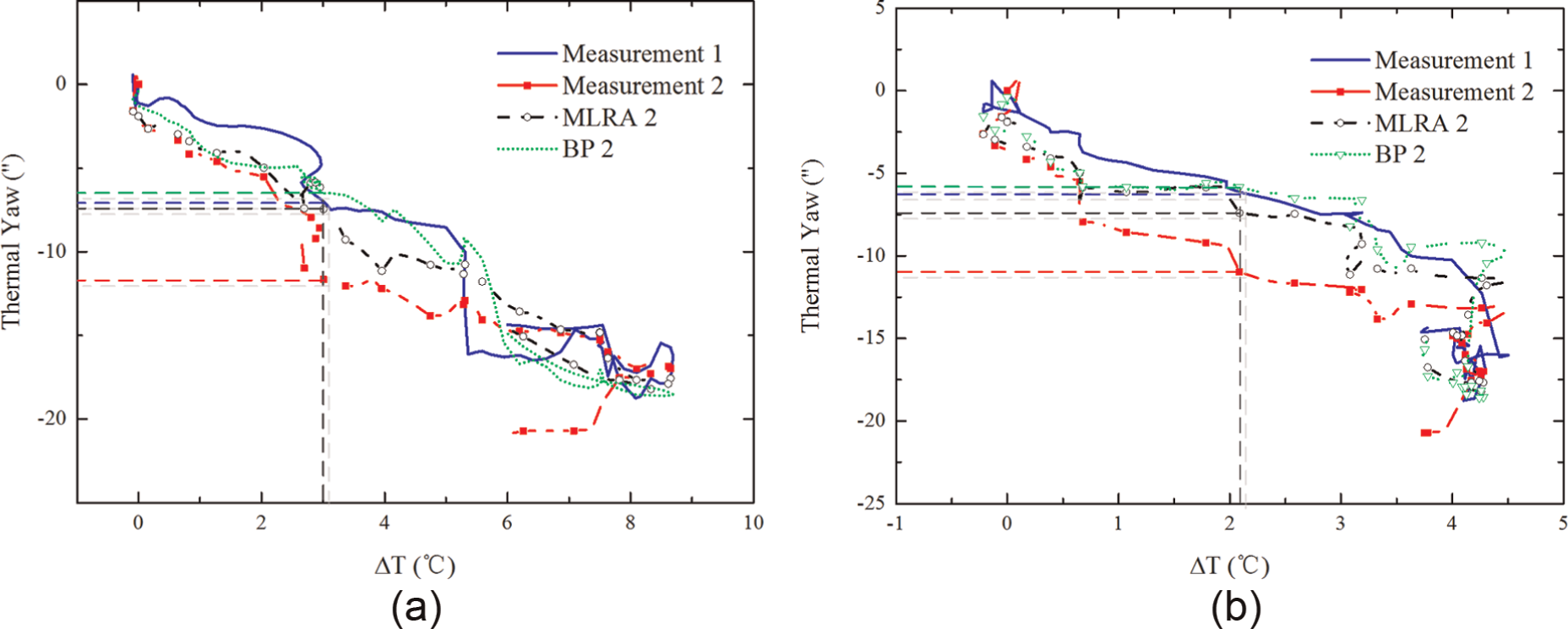
Radial thermal yaw angle error with temperature: (a)
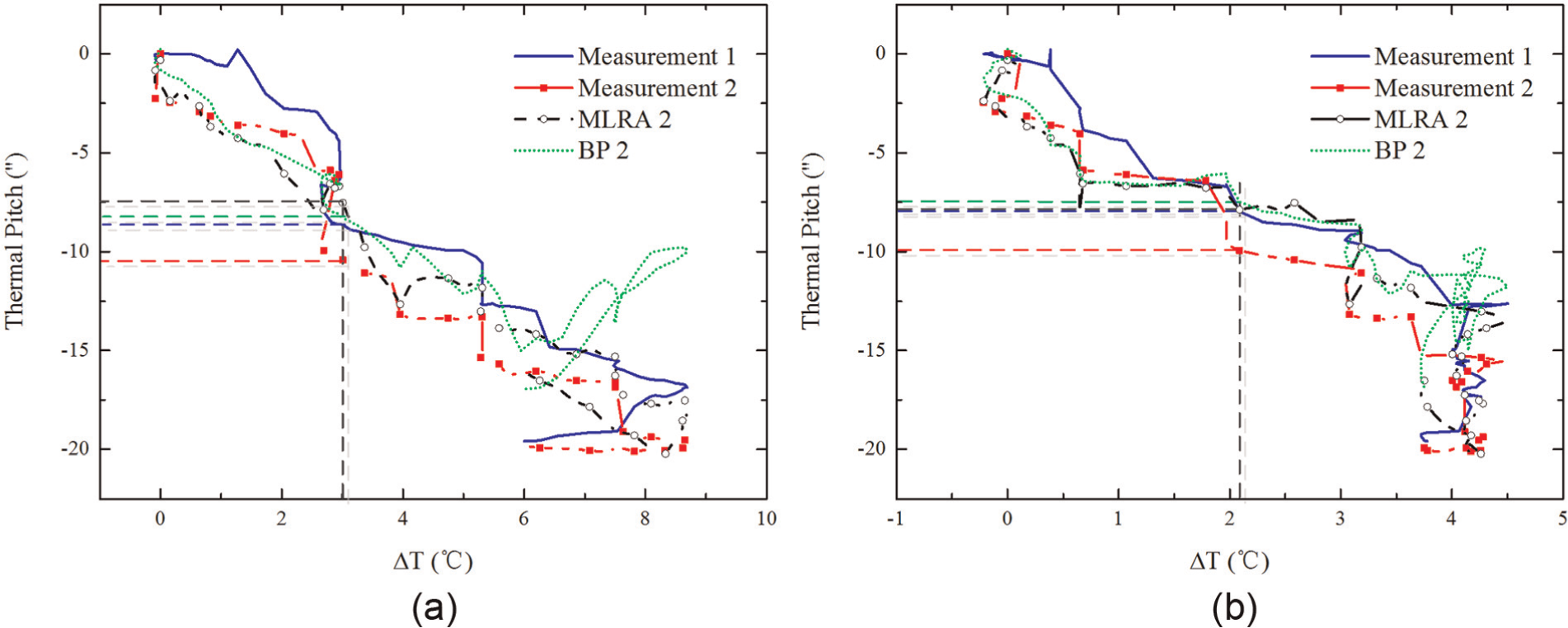
Radial thermal pitch angle error with temperature: (a)
In condition 2, when t = 165 min, the temperature rises of the rear/front bearings are
Comparison between the measured and the predicted results at
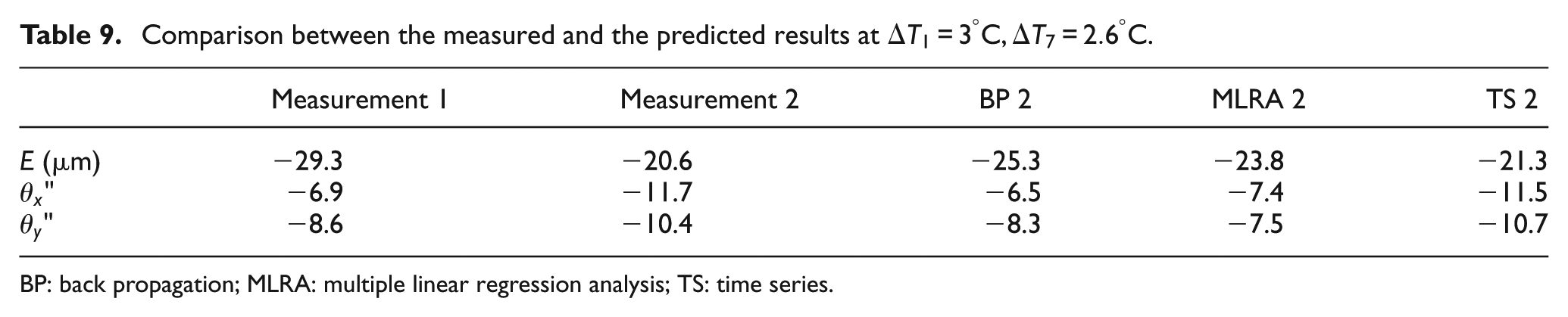
BP: back propagation; MLRA: multiple linear regression analysis; TS: time series.
The BP neural network has a strong nonlinear mapping ability, but its physical explanation is weak, its predictive ability is heavily dependent on the typical training samples, and the approximation and generalisation ability of the BP model are closely related to the typicality of the learning samples. When the sample changes, the predictive ability decreases. Fortunately, the TS model has no temperature variables, thus avoiding this difficulty.
2. The intrinsic properties of thermal errors on machines fitted by the TS model.
The thermal errors of the spindle are low-frequency signals that change slowly, show an increasing trend in processing due to the temperature rise and grow approximately linearly. Meanwhile, influenced by cooling fluid, heat conduction inside the shaft and air convection, there is a fluctuation with a certain periodicity in the series of the thermal error, which is obviously nonlinear. Moreover, the thermal error sequence is a random process that is influenced by outside factors, such as environmental temperature, radiation and vibration of the machine, so that the series of the thermal error inevitably contains random noise. In summary, the thermal error series usually includes three parts: a trend term, a periodic component and random elements, and Figures 10(a), 11(a) and 12(a) and Figures 14(a), 15(a) and 16(a) show these features clearly.
The
3. The nonlinear relationship between the temperature rise and the thermal error is an important consideration in model selection.
The machine thermal error is nonlinear not only in the time domain but also in the relationship with temperature rise,
4. The hysteresis effect of the thermal error has a great impact on the selection of the model.
Because an effect follows its cause, the change in thermal deformation of the spindle lags behind changes in the temperature field. In the case of thermal elongation, the experimental data are
This conclusion was proven in the experiment. While the spindle speeds decreased, as shown in Figures 4 and 13(b), the dissipated heat of the spindle was greater than the generated energy, so the temperatures declined slightly, while the thermal deformations continued to increase slowly, as shown in Figures 17–19. Both BP and MLRA only consider the present temperatures and thermal errors, ignoring the delayed effect between them, so the two models do not fully express the essential hysteresis characteristics of the thermal errors. Contrasting finely with BP and MLRA, the TS model reflects the dynamic dependency of the thermal errors series by the following equation

5. TS model can better characterise the cumulative effect of the thermal errors.
The acquired thermal error at each moment in the experiment is the accumulation of the thermal errors at the previous stage; namely, there is an intrinsic dependency between adjacent observations.
6.
TS in practical engineering are commonly non-stationary, which can be realised as a stochastic process. The thermal drifts and temperatures of the spindle in this article are no exception, and they are proven to be non-stationary series by the ADF test algorithm (ADF).
In this article, when the original sequences
In summary, the most important feature of MLRA is that the model has a simple structure with ordinary prediction accuracy, although the adaptive ability of the model is not strong and not suitable for nonlinear problems. The BP neural network has a strong nonlinear mapping ability, but it depends heavily on the training samples, and the approximation and generalisation abilities of the network model are closely related to the typicality of the learning samples. If the difference between new experimental samples and the sample for estimating the parameters of models is great, the predictive accuracy values of BP and MLRA are poor.
The TS analysis provides a set of approaches to process dynamic data. The basic idea of the TS analysis is that a mathematical model, which accurately reflects the system dynamic dependency, is established through the analysis of the time sequence samples based on a limited sample of the observation system. The method’s primary meaning is that all types of data are approximately described by mathematical models. Through the model analysis, the internal structure of the thermal error series can be mined so that we can forecast its trends and apply necessary controls to it. Hence, the TS model can adequately reflect the dynamic characteristics of the spindle thermal error, and it has excellent generalisation ability under different conditions.
Thermal error compensation
Cutting tool compensation offset
Figure 20 shows the thermal drift of the spindle in plane XOZ, with the spindle parallel to the Z-axis. During the experiments, the deviation mainly arose from spindle deformation due to the slight temperature rise of the detection probe. Therefore, it can be approximately considered that there were no changes in the shape of the probe and the tool. Supposing that the detecting probe was AP, where P was the end and the probe had length L, the displacement sensors S
1 and S
3 in the X-direction were placed at points B and H, respectively, with a distance between them of D, but the measurement point S
3 was not at the end of the probe. AT represents the handle. After the spindle deformed, the location of the probe translated to
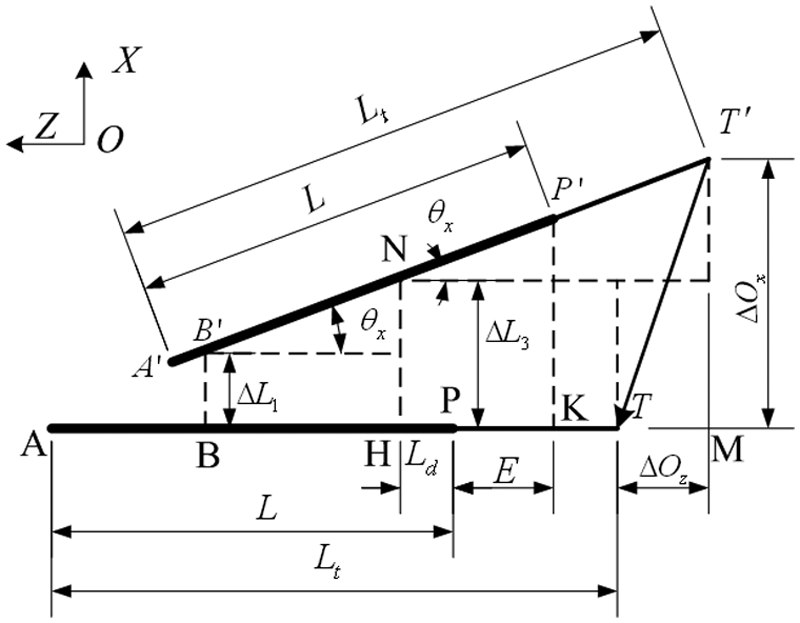
Thermal error offset map of the cutting tool.
The experimental results showed that the spindle expanded in the negative Z-direction after being heated and elongated from point T to M, so that the thermal offset of the cutting tool tip in the Z-direction was

where
Because the thermal yaw angle was small (i.e.


This indicates that the thermal offset of the cutting tool in the Z-direction was not related to the length of the tool.
The thermal offset of the cutting tool in the X-direction was

The thermal yaw angle was small, so

Applying equation (60) to equation (59), the thermal offset of the tool in the X-direction can be obtained

where
Similarly, the thermal offset of the cutting tool in the Y-direction

For

where
Because the thermal offsets of the tool in the X-, Y- and Z-directions were all negative, we can set the vector

Assuming that the original coordinate value of point W on the workpiece is

That is
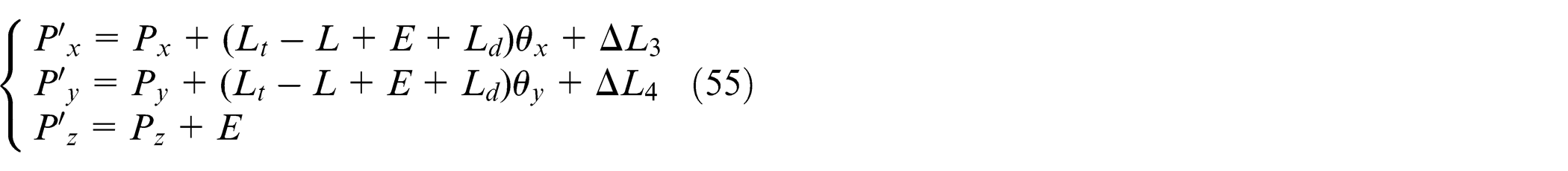
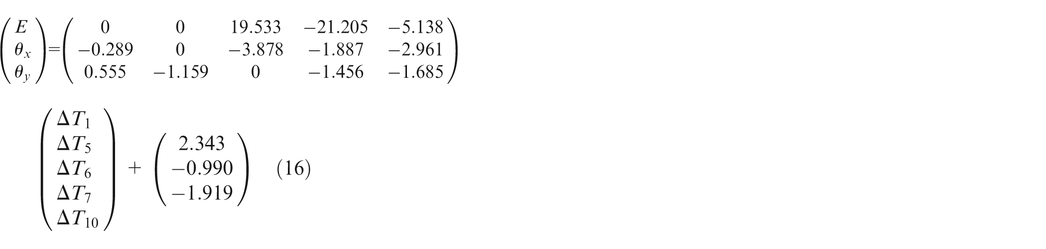
The spindle axial thermal elongation E, radial thermal yaw angle
Real-time compensation control
A sketched map of the spindle thermal error compensation is provided in Figure 21, and the CNC system is the Siemens 840D. The compensation system is composed of three parts: the processing module, HMI interface and PLC compensation module. The processing module acquires the temperatures and displacements from the sensors installed on the machining tool and can establish the thermal error model. While the real-time compensation is carried out, this module can calculate the thermal offsets and send the ultimate compensation values to the HMI based on the 840D secondary developments. Subsequently, the offsets are accepted by the PLC, and the offset value is inserted into the processing instructions to implement compensation for the thermal errors.
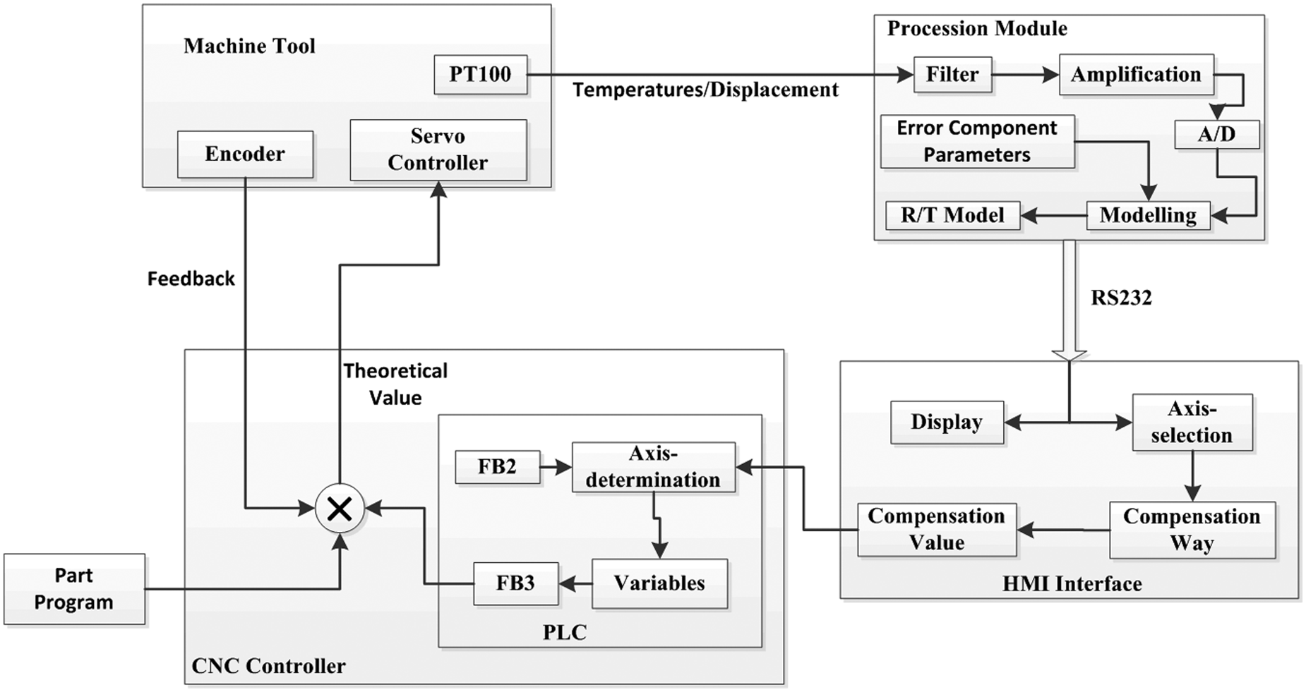
Thermal error compensation control.
Compensation result
The spindle thermal error compensation is implemented in three directions, and Figures 22–24 show the comparison of the measured value of the thermal error before and after compensation. After compensation in the X-direction, the displacement sensor S
3 is measured again and compared with the measurements before compensation. Similarly, displacement sensor S
4 in the Y-direction is compared before and after compensation, while the compared object in the Z-direction is S
5. The compensation parameters of the three models are shown in Table 10. Maximum and mean are the maximum and average absolute value of the thermal error after thermal compensation, respectively, and
Compensation in the X-direction.
Compensation in the Y-direction.
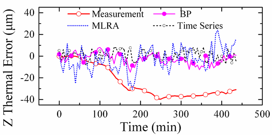
Compensation in the Z-direction.
Compensation result.
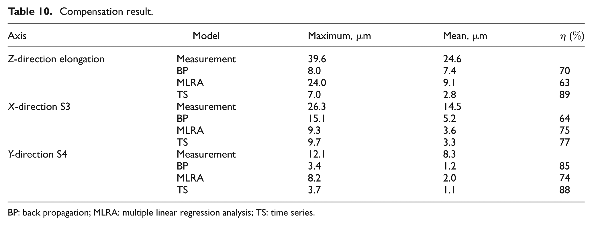
BP: back propagation; MLRA: multiple linear regression analysis; TS: time series.
Table 10 indicates that the TS model performed better than BP or MLRA. After compensation for the thermal errors, the error was reduced significantly in the axial direction. For TS, the maximum error decreased from 39.6 to 7 µm in the axis, and the average error decreased from 24.6 to 2.8 µm. The axial accuracy improved by 89%, which effectively demonstrates the proposed measurement and modelling method. BP and MLRA improved the accuracy by 70% and 63%, respectively. The absolute average value of the thermal error S 3 decreased from 14.5 to 3.3 µm in the X-direction, and the accuracy improved by 77% based on TS. In contrast, BP could improve the accuracy by 64% in the X-direction, while MLRA improved it by 75%. The accuracy was enhanced by 88%, 85% and 74% in the Y-direction using TS, BP and MLRA, respectively.
Conclusion
In this article, three types of thermal-induced error models with prediction-goodness evaluation criteria were constructed, with the aim of solving the problem that traditional spindle thermal error compensation ignores the radial tilt angle errors and the cutting tool length and does not improve the accuracy of the spindle in three dimensions. The error offsets in three directions were compensated with perfect accuracy improvement. A system of technical solutions was proposed for the measurement, modelling and compensation of the thermal error.
A synchronous acquisition system was developed, including a thermal deformation collection unit based on five eddy current displacement sensors and a multi-point temperature measurement unit with platinum resistance, which could simultaneously obtain real-time status information of the position-pose of the thermal error and the temperatures of the critical points. This information provides an in-depth analysis of the thermal behaviour of the motorised spindle. In addition, the five-point measurement method could effectively analyse changes in the axial expansion and radial thermal tilt angle errors.
A comprehensive thermal offset equation was presented, considering the radial tilt angles, elongation and cutting tool length, which can accurately describe the real position and pose of the spindle thermal deformation and efficiently improve the machine accuracy through compensation.
A compensation module was developed, and the compensated strategy was provided based on the feedback integral method and the secondary development of Siemens 840D, realising real-time on-line compensation.
A novel method was proposed to group temperature variables, using fuzzy cluster theory to packet temperature variables, and typical temperature variables were selected through statistical correlation analysis. This method can improve the efficiency of the model prediction with minimum independent variables and reduce modelling costs. Comparison of the three thermal error models demonstrated that the BP neural network has a desired fitting ability, but its generalisation is far less than that of the TS model. While the traditional MLRA model has a simple structure, it is a compromise choice between forecast accuracy and modelling cost. In contrast, the TS model can fully exploit the inherent dynamic characteristics of the thermal errors, which is more suitable to be used on the spindle thermal error compensation.
Footnotes
Declaration of conflicting interests
The authors declare that they have no financial and personal relationships with other people or organisations that can inappropriately influence our work; there is no professional or other personal interest of any nature or kind in any product or company that could be construed as influencing the position presented in, or the review of, the article.
Funding
This research was supported by the National High-Tech R&D Program of China (863 Program) under Grant Number 2012AA040701.