
Abstract
In this study, material removal rate (MRR) and surface roughness (Ra) in electrical discharge machining process have been modeled to make the process more efficient and reliable. First, adaptive neuro fuzzy inference system as one of the most used methods has been applied for prediction of material removal rate and Ra. Also a proposed method, that is, nonlinear modeling by system identification, has been applied to predict material removal rate and Ra. A group of electrical discharge machining experiments considering four input variables was conducted to collect dataset for training the predictive models. At the end, the comparison of predicted results from both approaches with experimental data shows that the new method has a much better performance than the adaptive neuro fuzzy inference system approach.
Keywords
Introduction
Electrical discharge machining (EDM) is a nontraditional manufacturing process which has been extensively applied to machine conductive hard-to-cut materials (like super alloys) regardless of their hardness and some other physical properties such as elasticity modulus and thermal capacity.1–3 The material removal mechanism of the process is based on electro-thermal effect of electrical discharge phenomena frequently occurred between the two nearest lumps located on two electrodes with opposite polarity which submerged in insulated dielectric fluid.4,5
Due to complex and stochastic nature of EDM process, it is still a disputable problem to establish a robust model denoting accurate relationships between controllable input variables and output parameters.6–8 That is the reason why so many efforts with different approaches such as statistical analysis based on design of experiments, artificial neural networks (ANN) and fuzzy logic and adaptive neuro fuzzy inference system (ANFIS) have been carried out to model, analyze, optimize and predict EDM process performance.6,8–13
In order to contribute the knowledge and experiences of the experts, applying fuzzy logic–based techniques could be a reliable technique to model and optimally control the process. To reach machining stability and improvement in performance index (machining speed, depth of cut) a fuzzy inference system with only two input signals including frequency of short circuit and arcing was employed by Kaneko and Onodera. 14 They introduced a self-adjusting fuzzy controller using jumping height and approaching movement of electrode to avoid abnormal states in EDM process.
Tsai and Wang 15 compared six models based on ANN with an ANFIS model and their results illustrating the superiority of ANFIS model for predicting MRR (16.33% error). They concluded that ANFIS model using generalized bell (G-bell) membership function (MF) in input variables would result in the best results. In order to predict the white layer thickness and the average surface roughness (Ra) in wire electrical discharge machining (WEDM) process, Çaydas et al. 16 ran a full factorial design that consists of 24 experiments. Pulse duration, open circuit voltage, dielectric flushing pressure and wire feed rate were considered as four input variables. They applied ANFIS models using Gaussian MF in input variables. To evaluate ANFIS models, eight test cases extracted from 24 experimental data were chosen for simulation. Maji and Pratihar 12 presented models of EDM performance by statistical approach based on response surface methodology and ANFIS. The modeling based on ANFIS was conducted in two directions: forward and reverse mapping. Two types of fuzzy MFs, including triangular and generalized bell MFs, were used in ANFIS models. Because of nonlinear inherent of EDM process, ANFIS models using G-bell MF displayed more accurate results compared to ones using triangular MF for predicting MRR and Ra. Artificial data obtained from regression equations of output characteristics were used for optimal training of ANFIS models. Majumder 17 conducted a comparative study to model and optimize EDM process parameters. Three evolutionary algorithms including simulated annealing, genetic algorithm and particle swarm optimization (PSO) were coupled with neural network model. These three evolutionary algorithms used well-trained back-propagation neural network (BPNN) model as a fitness function. Through this investigation, PSO integrated that BPNN model was found more accurate to predict the optimal process parameter for maximum machining performance.
From the literature survey, obviously most of the neural network–based approaches explained so far had used a recursive structure such as ANN and ANFIS. Beside some drawbacks, recurrent neural networks, because of their intrinsic nonlinearity and computational simplicity, are natural candidates to approximate a given model for such a stochastic-natured process like EDM. However, system identification approach as one of the widely employed methods for prediction purposes, including such convenient model forms for prediction purposes like the nonlinear autoregressive model with exogenous variables (NARX) 18 and Hammerstein–Wiener (HW) model, 19 has not been employed before, to the authors’ knowledge, for EDM performance prediction. The success of NARX and HW models is due to both their capability of capturing nonlinear dynamics and the availability of identification algorithms with a reasonable computational cost.20,21 These two are a powerful class of models which has been demonstrated that they are well suited for modeling nonlinear systems.22,23
In this study, ANFIS, as one of the most used and a new approach, that is, nonlinear modeling using system identification, has been employed to build predictive models of EDM performance. The main goal of the current work, beside an enhancement of ANFIS model’s capability through artificial data, is to compare the predictive performance of ANFIS approach with the NARX and HW models and to illustrate that the presented approach is reliable and has much higher accuracy than other common method (such as ANFIS) in order to predict characteristics such as MRR and Ra. To compare the results, all conditions for ANFIS and system identification methods are set to be identical—including input variables and training data. This article is structured as follows: in the next section, brief review of ANFIS, NARX and HW concepts is presented. In section “Experimental setup and method,” experimental setup and method is presented. In section “Results and discussion,” prediction results are presented and then discussed. Finally, conclusions are presented.
Basic theory
In this section, a brief review of ANFIS and system identification concepts for predicting output characteristics is presented.
ANFIS
ANFIS was developed by Jang 24 to minimize an output error measure and maximize cost index. As shown in Figure 1, ANFIS is a multilayered feed-forward neural network based on Sugeno fuzzy inference system which has been widely applied for modeling, predicting and controlling of stochastic and nonlinear processes. ANFIS concurrently uses fuzzy reasoning and neural network calculation to establish mapping relation from input variables to output parameter. 19 Faster convergence, smoothness, adaptability, smaller size of the training set and optimization search space are the main advantages of using ANFIS rather than neural networks and fuzzy systems.25,26 In order to tune adaptive parameters of ANFIS, training of network and optimal distribution of MFs are executed by hybrid learning algorithm composed of least squares estimates and back-propagation error to perform forward pass and backward pass, respectively.
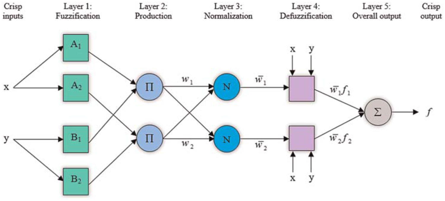
ANFIS architecture.
An MF is a curve that defines how each point in the input space is mapped to a membership value between 0 and 1. There are different types of MFs; here, three of the most common MFs which are utilized in this study are introduced in the next subsections.
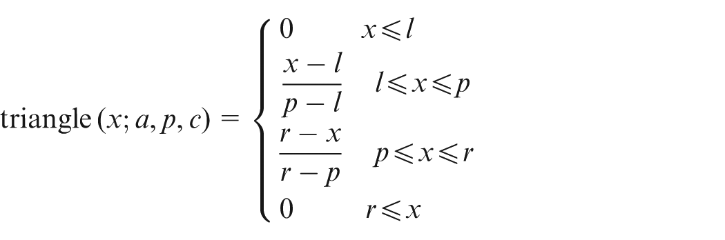
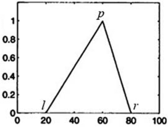
Triangular-shaped MF
The triangular curve is a function of a vector x and can be defined by three parameters, left point (l), peak point (p) and right point (r), as follows
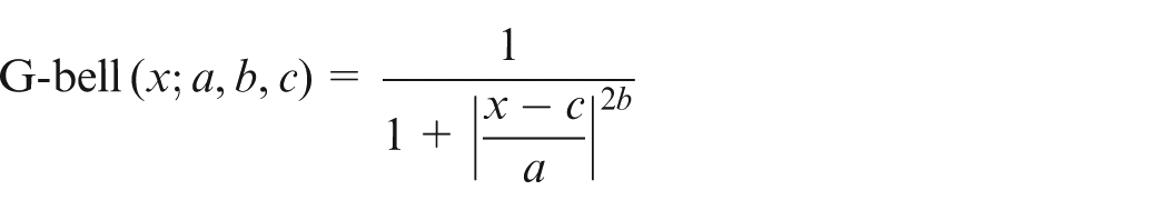
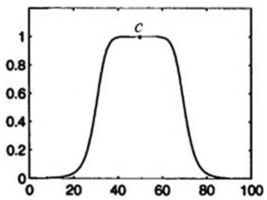
Generalized bell-shaped MF
The G-bell function is a symmetric curve that depends on three parameters a, b and center of the curve (c) as given by
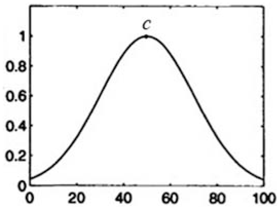
Gaussian curve MF
The Gaussian MF function is a symmetric curve that can be defined by two parameters, MF’s width (w) and MF’s center (c), as follows

System identification
NARX
NARX models are the nonlinear generalization of the well-known autoregressive exogenous (ARX) models, which constitute a standard tool in linear black-box model identification. 27 These models can represent a wide variety of nonlinear dynamic behaviors and have been extensively used in various applications.22,23,28
Typically, the NARX models will be used as black-box structures and have a structure as equation (1)
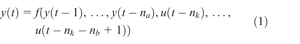
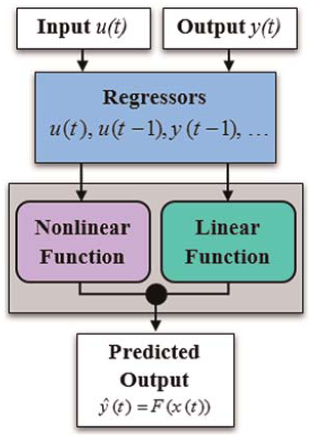
where the function f depends on a finite number of previous inputs u and outputs y. na is the number of past output terms and nb is the number of past input terms used to predict the current output. nk is the delay from the input to the output, specified as the number of samples. The NARX model uses a parallel combination of nonlinear and linear blocks. NARX model structure is shown in Figure 2. The NARX model uses regressors as variables for nonlinear and linear functions. Regressors are functions of measured input–output data. The predicted output

where
where
NARX model structure. 23
The NARX model computes the output in two stages:
Computes regresses from the current and past input values and past output data.
The nonlinearity estimator block maps the regresses to the model output using a combination of nonlinear and linear functions.
HW
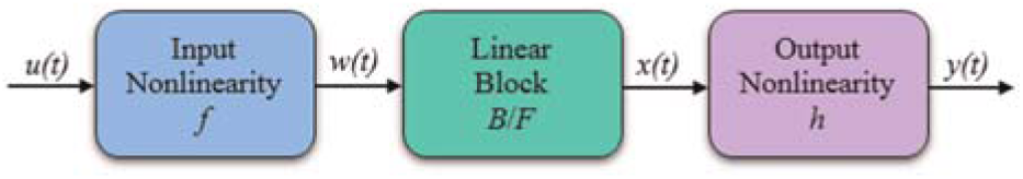
HW model describes linear systems surrounded by an input and an output static nonlinearity as shown in Figure 3. This block-oriented nonlinear model has been studied for some time now 19 and has also been used for modeling and prediction purposes.23,30 The HW model can be used as a black-box model structure because it provides a flexible parameterization for nonlinear models. 25
Hammerstein–Wiener model structure.
where w(t) = f(u(t)) is a nonlinear function transformation input data u(t); w(t) has the same dimension as u(t); x(t) = (B/F)w(t) is a linear transfer function; x(t) has the same dimension as y(t); B and F are the backward shifting operators.
For ny outputs and nu inputs, the linear block is a transfer function matrix containing entries
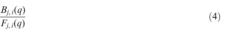
where j = 1, 2, …, ny and i = 1, 2, …, nu; y(t) = h(x(t)) is a nonlinear function that maps the output of the linear block to the system output; w(t) and x(t) are the internal variables that define the input and output of the linear block, respectively.
Because f acts on the input port of the linear block, this function is called the input nonlinearity. Similarly, because h acts on the output port of the linear block, this function is called the output nonlinearity. The nonlinearities f and h are scalar functions, one nonlinear function for each input and output channel. The linear block setting [nb, nf, nk] sets the order of the linear transfer function, where nb is the number of zeros plus 1, nf is the number of poles and nk is the input delay.
The HW model computes the output y in three stages:
Computes w(t) = f(u(t)) from the input data. w(t) is an input to the linear transfer function B/F;
Computes the output of the linear block using w(t) and initial conditions: x(t) = (B/F)w(t−nk);
Computes the model output by transforming the output of the linear block x(t) using the nonlinear function h: y(t) = h(x(t)).
The input and output nonlinearities can be configured as a sigmoid network, wavelet network, saturation, dead zone, piecewise linear function and one-dimensional polynomial.
Experimental setup and method
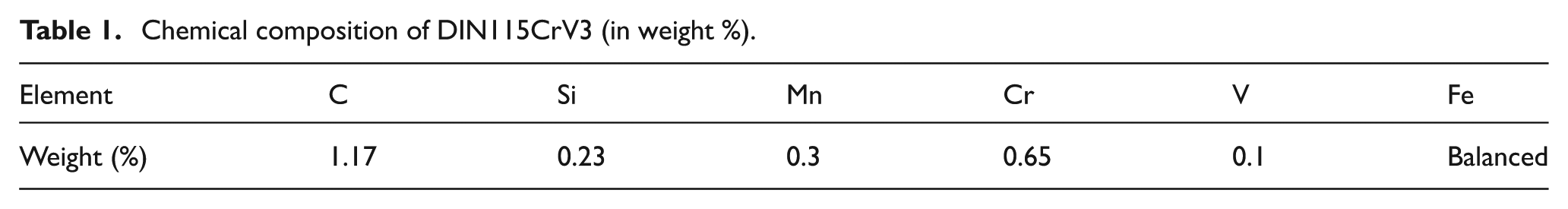
Anorak spark erosion 20 A machine was employed to perform the experiments. In this study, ISO-frequency pulse generator mode was employed to conduct the experiments. Commercial pure copper with wide application and access was chosen as the tool electrode material. The steel DIN115CrV3 with a density of 7.8 g/cm3 and commercial kerosene oil were selected as a workpiece material and dielectric medium, respectively. Table 1 lists the chemical composition of DIN115CrV3. Cylindrical shape with 10 mm diameter and 40 mm length was selected for both electrode tool and workpiece. Due to the cylindrical shape of the workpiece, a chuck was installed on the bottom surface of the EDM machine tank to clamp the workpiece. A total of 10 min was assigned as machining time for each setting of the experiments.
Chemical composition of DIN115CrV3 (in weight %).
Planning of experiments was conducted based on a mixed-level design to establish the input–output relationships in EDM process. The input variables and their values are given in Table 2. MRR and Ra were considered as output features. A total of 60 number of experiments was determined by multiplying corresponding levels of input variables. Also, eight new settings of experiments with different input variable levels from those of main data (including 60 settings) have been employed as a test case to evaluate each predictive model’s prediction accuracy.
Process input variables and their levels.
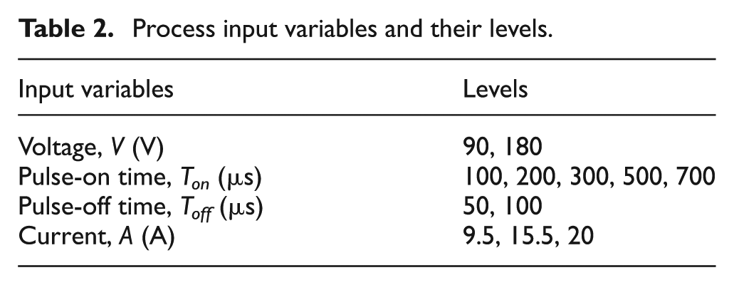
The corresponded input level values in Table 2 are the most extensively used ranges which are widely applied in the industry. Since the industrial operating conditions include various settings, in order to astutely evaluate the model’s predictive performances, these eight test cases’ input values were selected between the corresponded ranges of input variable levels reported in Table 2; while some researchers had chosen some data as test data which are extracted from the main data.11,15
MRR was calculated by means of changing the mass before and after EDM operation utilizing a digital single pan balance with maximum capacity of 210 g having a resolution of 1 mg. The following equation was employed to calculate the volume of MRR
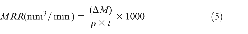
where
Results and discussion
In this section, the models based on ANFIS, NARX and HW for predicting MRR and Ra are presented. To investigate the performance of the obtained models, various criteria have been used to compare performances and calculate the errors. To design ANFIS models, number and type of MFs have a key role. Through applying various linear and nonlinear MFs, triangular, generalized bell and Gaussian MF that have displayed better performance have been selected to establish ANFIS models. Various numbers of MF have been tried for each input variable, which resulted to allocate 2, 5, 2, 3 MF for voltage, pulse-on time, pulse-off time and current, respectively. Hence, ANFIS models based on 2 × 5 × 2 × 3 = 60 fuzzy rules were established as shown in Figure 4. The hybrid learning algorithm was employed for training ANFIS predictive models. All the predictive models were designed after 100 epochs.
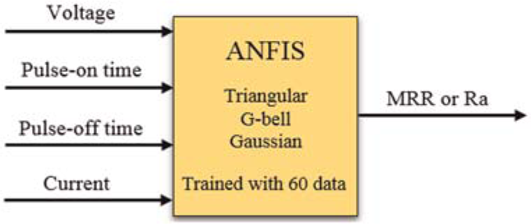
ANFIS model structure.
Configuration of the developed ANFIS models is same as the previous ANFIS models. It means that these models have been designed and constructed utilizing triangular, G-bell and Gaussian MF with 60 fuzzy rules as shown in Figure 5. Also, the hybrid learning algorithm was employed for training, and all models were designed after 100 epochs.
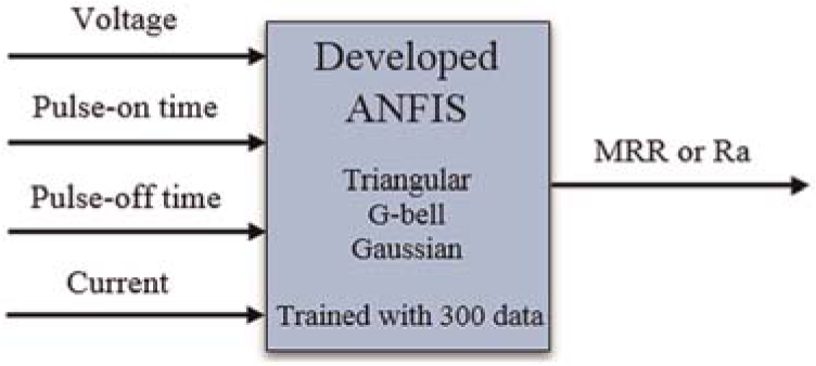
Developed ANFIS model structure.
Two groups of dataset have been used to construct the ANFIS models. The first one consists of 60 experimental data and the second one consists of 300 data that comprises 240 artificial data and 60 experimental data. The first group of the dataset was employed to train ANFIS models, while the second group of the dataset was employed to train the developed ANFIS models.
The 240 artificial data in the second dataset were generated by regression equations. The regression equations were obtained using Minitab 16 software. To achieve the best results, several regression equations for MRR and Ra were tested. Finally, based on residual analysis and adjusted correlation coefficient, best results were obtained from the following equations
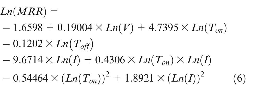
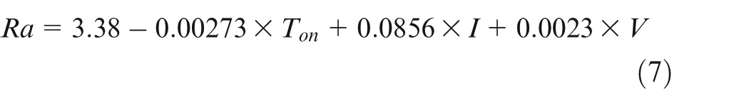
where V, Ton, Toff and I represent the voltage, pulse-on time, pulse-off time and current, respectively.
At this stage, the performance of the obtained models, ANFIS and developed ANFIS, will be investigated through simulation. To assess this, output results of these models from prediction of the eight blind test data of MRR and Ra are compared with the real ones. First, the comparison is done in the form of coefficient of determination (R2) which is calculated according to equation (8)
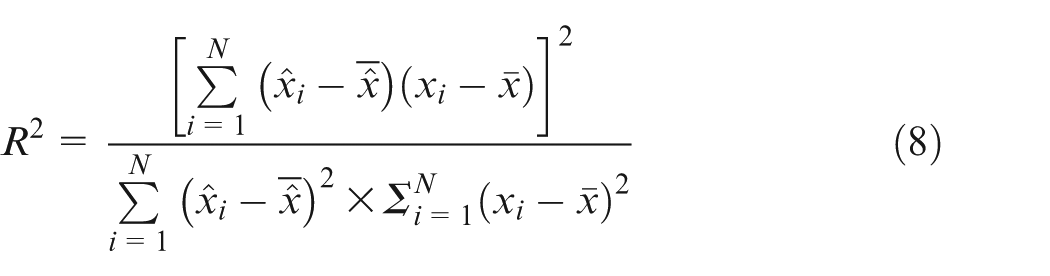
In this equation,
As mentioned in the previous section, in the test data, there are some data settings with different range values from the experimental dataset, since the industrial operating condition includes enormous setting. Therefore, to attain a reliable and accurate model of the process performance, such model must be capable of accurately predicting different level of the industrial operating setting. And also that the test data have not been seen by the models. Hence, the best predictive model is the one that is well trained and can better map the relationship between inputs and outputs. Such model can accurately predict all the outputs, even those output that have different range values. Figure 6 shows the R2 results of the ANFIS and developed ANFIS models for MRR prediction.
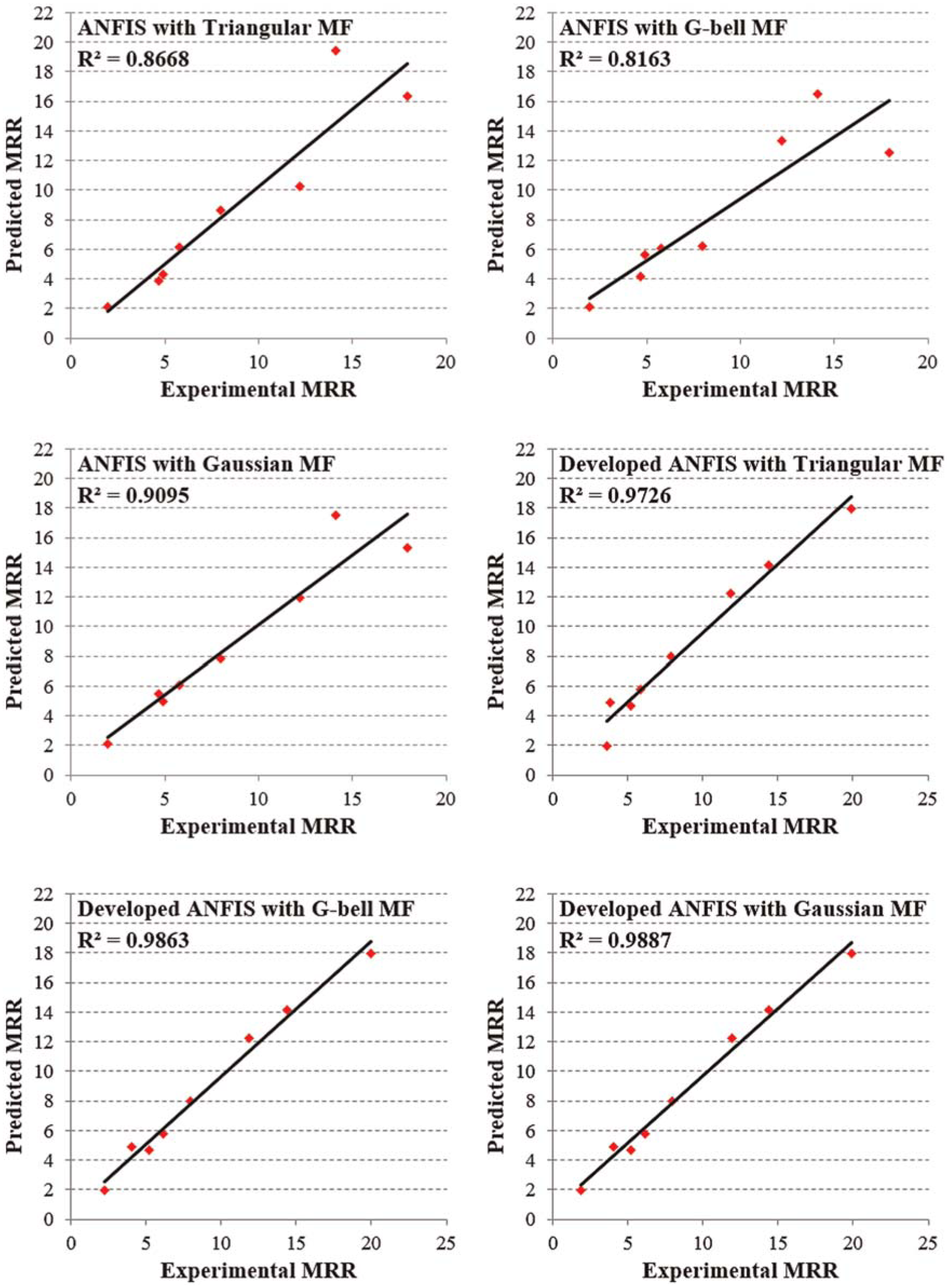
R2 result of ANFIS and developed ANFIS models for MRR prediction.
As it can be seen from Figure 6, the best result from both ANFIS and the developed ANFIS models is achieved using Gaussian MF. This result indicates that the Gaussian MF has better performance to establish a mapping between inputs and output variable (MRR). An appealing result is that the performance of the models achieved from the developed ANFIS models was much better than those achieved from the ANFIS models. To illustrate more, even the best models resulted from the ANFIS models had a weaker performance in comparison with the models achieved through the developed ANFIS models. This outcome shows that the number of training data has significant impact on the performance of the ANFIS models. So, it is not necessary to have a large number of high-cost and time-consuming laboratory data. Instead, if required, additional data can be artificially generated.
In the next stage, performance of ANFIS approach for prediction of the Ra has been investigated. Figure 7 shows the R2 results of the ANFIS and developed ANFIS models for Ra prediction.
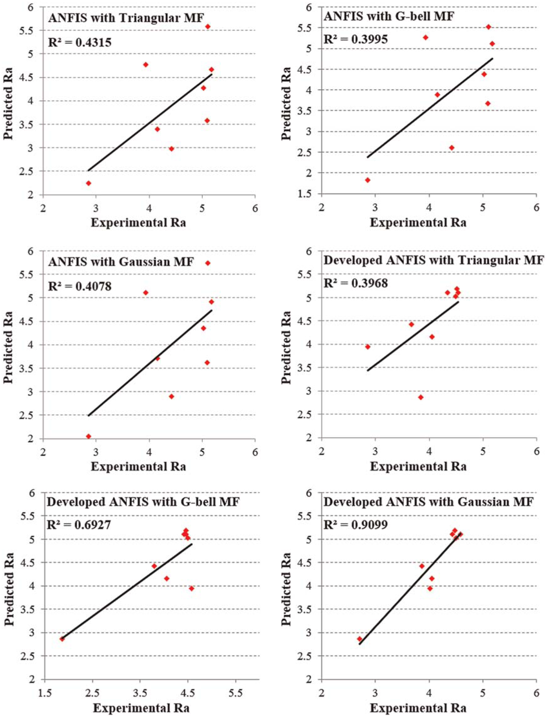
R2 result of ANFIS and developed ANFIS models for Ra prediction.
The results show that for the prediction of Ra, developed ANFIS models also surpassed the ANFIS models. So, the artificial data were well produced and had a positive effect on the models’ prediction performances. An interesting result is that in both cases of MRR and Ra prediction, the best result from ANFIS approach has been achieved using Gaussian MF.
Moreover, in the next step, the prediction of MRR and Ra is done with the system identification of nonlinear models, NARX and HW. In order to achieve best prediction results, various configurations have been considered for NARX and HW. At the end, with thorough review, the best models for MRR and Ra were selected. Same as ANFIS models, inputs of NARX and HW models are voltage, pulse-on time, pulse-off time and current, respectively. Moreover, all of the NARX and HW models were trained by employing 60 experimental data similar to the ANFIS models. Specifications of the best models for MRR and Ra are summarized in Table 3.
Specification of the selected NARX and HW models.
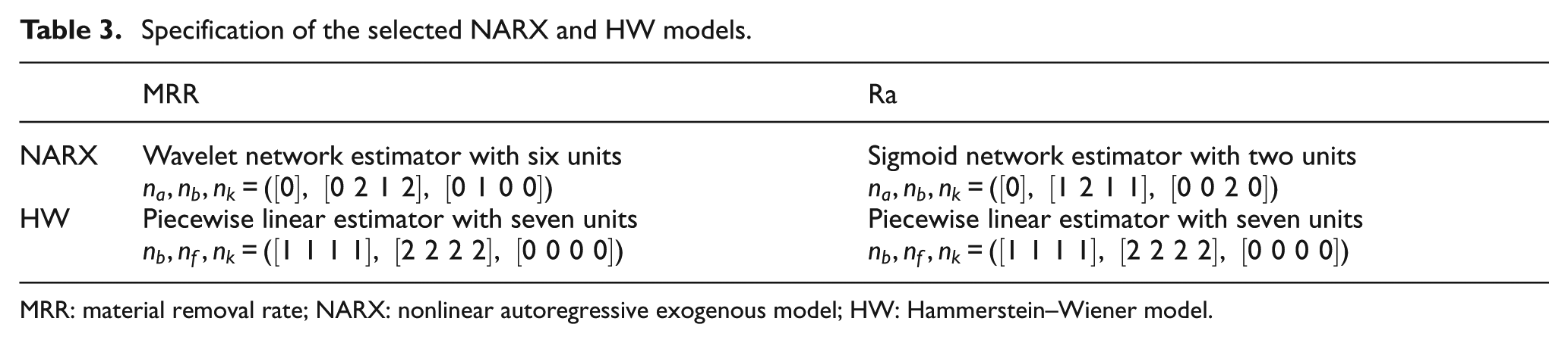
MRR: material removal rate; NARX: nonlinear autoregressive exogenous model; HW: Hammerstein–Wiener model.
Using R2 criteria, performance of the selected models is investigated. Figure 8 shows the R2 results of the NARX and HW models for MRR and Ra prediction.
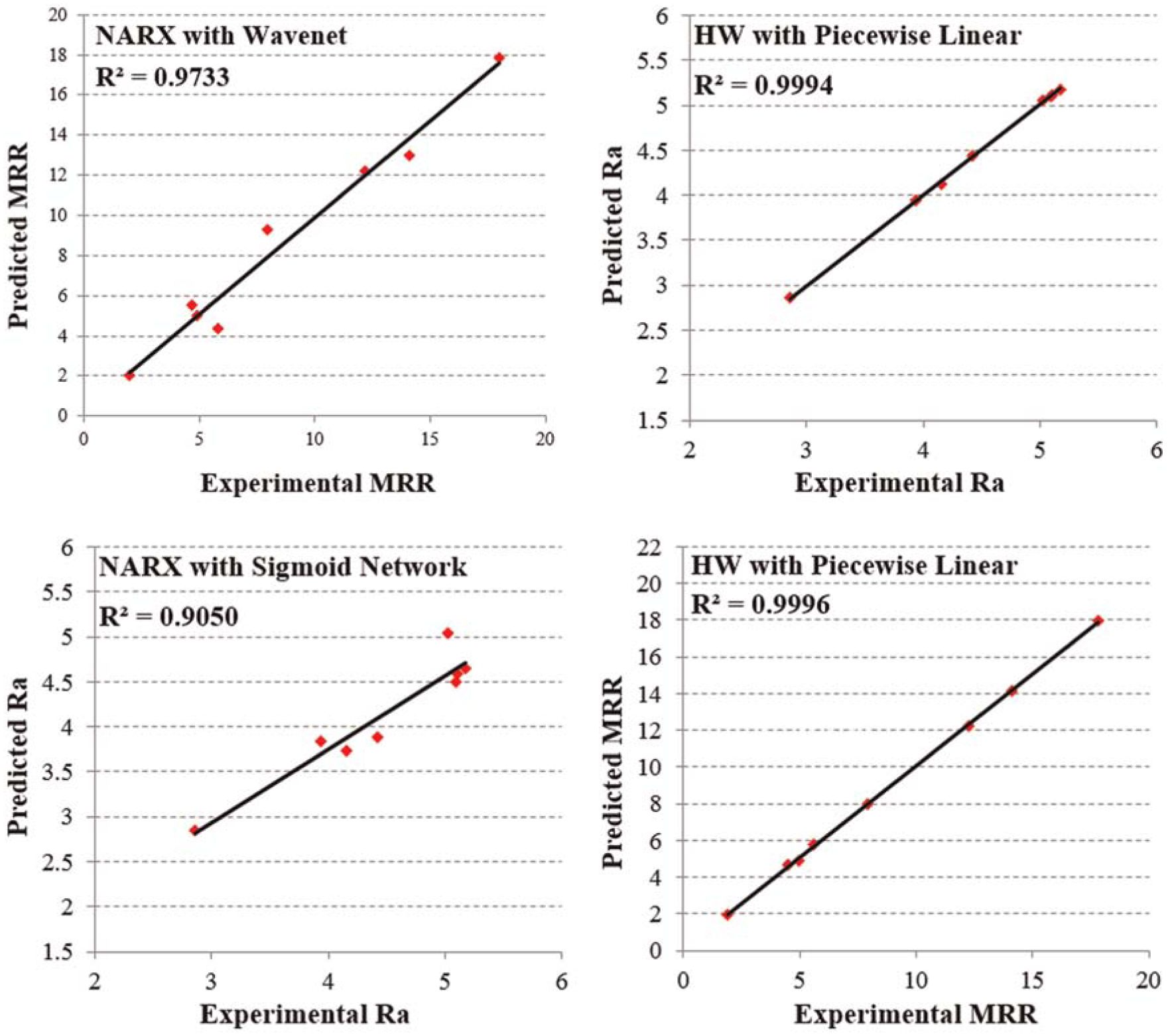
R2 result of NARX and HW models for MRR and Ra prediction.
As it can be seen from Figure 8, performance of the selected HW models is excellent in both cases of MRR and Ra prediction. Also, the performance of the NARX model for prediction of MRR is very good. It can be seen that the performance of the NARX model is almost equal to the best model from Figure 7. Of course, performances of NARX models are not as well as HW models. However, NARX model built for MRR used only three inputs (without using the first input data, i.e. voltage) and showed a satisfactory performance (as it can be seen from Table 3). It should also be noted that like ANFIS, NARX and HW models have just been trained with 60 experimental data. So, it can be concluded that the performance of the HW models is indeed excellent.
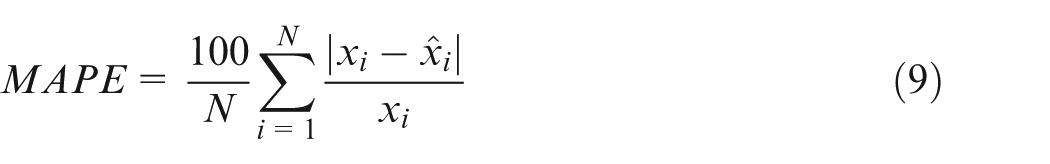
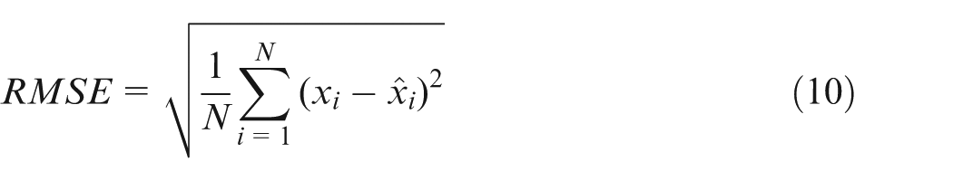
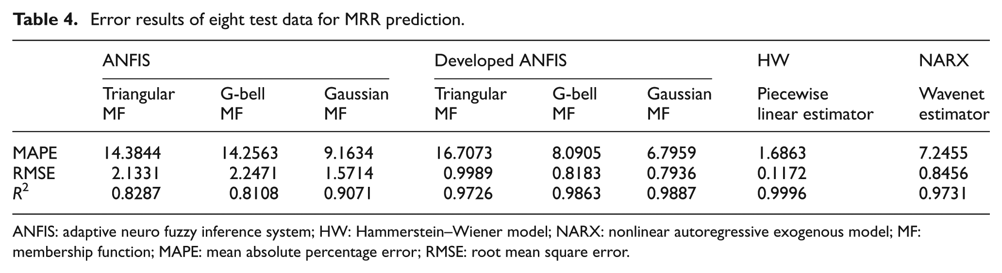
Moreover, to compare the performance of all the selected models, various criteria were used to calculate prediction errors. The criterion mean absolute percentage error (MAPE), according to equation (9), shows the mean absolute error that can be considered as a criterion for model risk to use it in real-world conditions. Root mean square error (RMSE), according to equation (10), is a criterion to compare the error dimension in various models. The errors of the obtained models for the prediction of MRR considering these error criteria are summarized in Table 4.
Error results of eight test data for MRR prediction.
ANFIS: adaptive neuro fuzzy inference system; HW: Hammerstein–Wiener model; NARX: nonlinear autoregressive exogenous model; MF: membership function; MAPE: mean absolute percentage error; RMSE: root mean square error.
As it can be seen from Table 4, the HW model has very low error values. This model predicted MRR values very accurately. Developed ANFIS model utilizing Gaussian MF for input variables is located in the second place regarding low error values. However, as it is said before, they have been trained by more data than the NARX model. Therefore, the performance of the NARX model could also be considered adequate for predicting EDM performances. It can be seen that the HW model shows an evident improvement at predicting MRR over the best ANFIS model.
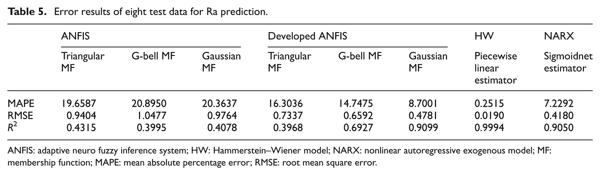
In the next step, performance of all the selected models in Ra prediction is investigated. Table 5 shows error results of the obtained models for the prediction of Ra considering error criteria (equations (8)–(10)).
Error results of eight test data for Ra prediction.
ANFIS: adaptive neuro fuzzy inference system; HW: Hammerstein–Wiener model; NARX: nonlinear autoregressive exogenous model; MF: membership function; MAPE: mean absolute percentage error; RMSE: root mean square error.
As the results of Table 5 shows, performance of the HW model for the prediction of Ra is also outstanding. It can be seen that just like MRR, the HW model shows an obvious improvement in predicting Ra over the best ANFIS model. Moreover, performances of the developed ANFIS model (with Gaussian MF) along with NARX model are acceptable.
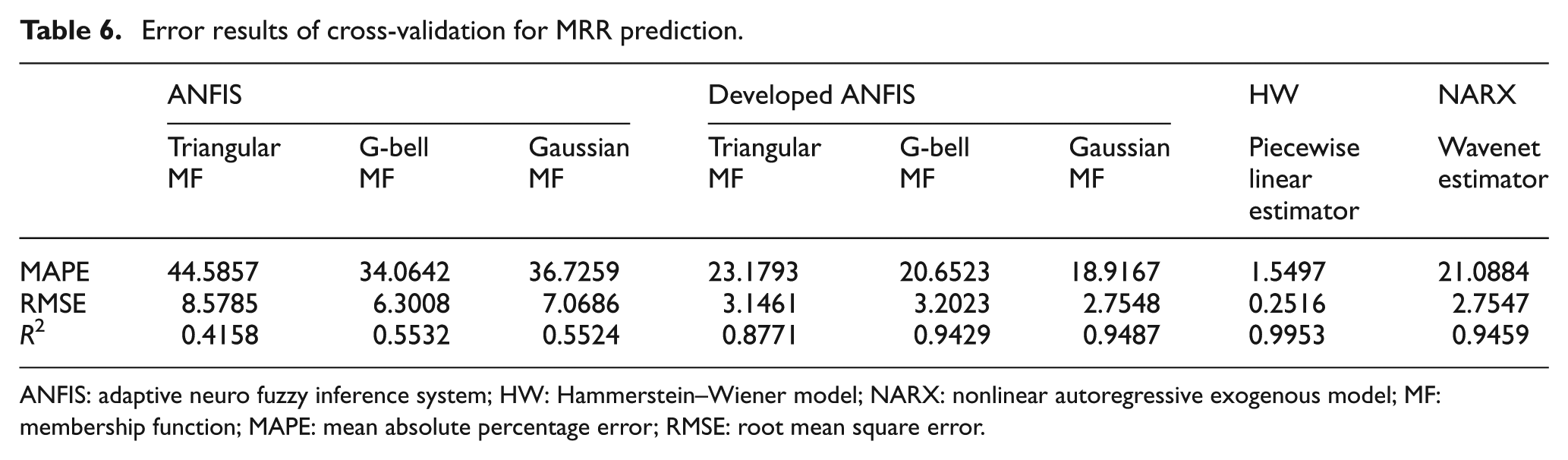
Finally, to achieve an unbiased estimation of the model performance, the dataset can be divided randomly into k subsets of equal size and k-fold cross-validation performed. In this method, models are built k times, each time leaving out a single subset as the validation data for testing the model and the remaining k − 1 subsets are used as training data. The k results from the folds are then averaged to yield a single result. Here, to maintain the ratio of test data similar to previous tests (Tables 4 and 5), each test subset is set to contain eight data. The dataset contains 68 data; thus, the dataset is randomly divided into nine folds in which each fold contains eight data. Since nine folds containing eight data result in 72 sample data, only in one fold, four duplicate data must be used. Tables 6 and 7 show the outputs for nine-fold cross-validation for MRR and Ra, respectively.
Error results of cross-validation for MRR prediction.
ANFIS: adaptive neuro fuzzy inference system; HW: Hammerstein–Wiener model; NARX: nonlinear autoregressive exogenous model; MF: membership function; MAPE: mean absolute percentage error; RMSE: root mean square error.
Error results of cross-validation for Ra prediction.
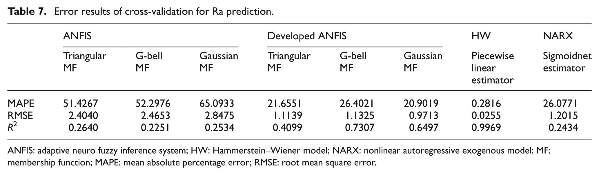
ANFIS: adaptive neuro fuzzy inference system; HW: Hammerstein–Wiener model; NARX: nonlinear autoregressive exogenous model; MF: membership function; MAPE: mean absolute percentage error; RMSE: root mean square error.
At the end, it can be seen from cross-validation results in Tables 6 and 7 that models from the system identification approach, especially HW models, have an excellent predictive performance of EDM characteristics. Hence, predicting MRR and Ra using HW model is a new approach to obtain higher prediction accuracy with lower computational cost. Also, the proposed approach needs less experimental data than ANFIS approach. Furthermore, if extra data are needed, using regression equations is an effective and suitable method instead of collecting another time-consuming and costly experimental dataset.
Conclusion
In this article, prediction of MRR and Ra characteristics in EDM process has been studied. For this purpose, two approaches were used, ANFIS and a proposed method, that is, nonlinear system identification. The required dataset for training the models was obtained through running experiments based on a design with mixed levels utilizing comprehensive analysis of variance. Then, using regression equations which were fitted on output responses, artificial data were obtained. Real experimental data and artificial data were used for training of ANFIS and developed ANFIS models, respectively, while NARX and HW models of system identification method were trained only by experimental data. Then, all models were compared with each other to evaluate their predictive performance. To accomplish this, some experimental data with different input variable values from training data were used as a test case, and performances of all the models for the prediction of the MRR and Ra were evaluated by various error criteria. Furthermore, cross-validation was performed to achieve an unbiased estimation of the model performance.
The evaluation of results and their comparison show that the obtained models from the proposed method, system identification, especially the HW models, have an outstanding predictive performance with higher accuracy than ANFIS models for both MRR and Ra. Also, the result shows the effectiveness of the artificial data on the performances of the developed ANFIS models. Therefore, instead of making a costly and time-consuming large dataset, required data can be artificially produced (e.g. by regression equations) that lead to proper and effective performance.
Footnotes
Declaration of Conflicting Interests
The author(s) declared no potential conflicts of interest with respect to the research, authorship and/or publication of this article.
Funding
The author(s) received no financial support for the research, authorship and/or publication of this article.