Sage Journals: Discover world-class research

Abstract

A numerical model based on computational fluid dynamics is developed to analyze fluid flow and thermal aspects in grinding. The model uses multiphase fluid flow with heat transfer based on the volume-of-fluid method, convection, conduction in solids and a multiple reference frame model of the porous grinding zone. Fluid velocity vectors, useful flow rate, grinding temperatures and energy partition are predicted using the model. In lieu of direct measurements of these quantities, the verification relies on the indirect assessment of surface integrity. The simulation results provide adequate agreement with the measured residual stress, depth of heat-affected zone and full width at half maximum profile with respect to the grinding temperatures.

Keywords

Grinding computational fluid dynamics thermal effects heat transfer surface integrity

Introduction

Grinding of high-speed steel (HSS) is difficult due to high workpiece hardness and wear resistance. The grindability of HSS is largely affected by the hard tungsten–molybdenum and vanadium carbides held firmly in the hardened-steel matrix.¹ These typically lead to high specific energies compared to grinding other steels, especially when using aluminum oxide wheels. This can lead to high workpiece surface temperatures, resulting in various types of thermal damage such as thermal softening (overtempering), residual tensile stresses, rehardening and cracking. Residual tensile stress and rehardening burn are particularly critical because they reduce service life and reliability of a workpiece operating under fatigue conditions.² It was found by Chen et al.³ that thermal loads generated in the grinding process are the primary source of tensile residual stresses. The most practical solution to avoid the onset of tensile residual stresses is to keep the grinding temperatures below the workpiece tempering temperature. Therefore, it is crucial that the grinding temperatures are readily known—either by direct measurements or by simulation.

A critical parameter for calculating the grinding temperatures using the moving heat source theory is the energy partition, which is the fraction of the specific energy transported as heat to the workpiece in the grinding zone.⁴ Typically, to determine the specific energy into the workpiece, grinding power is measured and specific energy is calculated using the material removal rate. Then, the energy partition is estimated, which requires considerable experimental effort. Different estimation techniques are discussed by Malkin and Guo.⁴ An alternative method of determining the specific energy into the workpiece involves measuring the depth of rehardening burn in ground workpieces and reverse-calculating the maximum surface temperature.⁵ This also requires time-consuming metallographic examinations. Therefore, a more straightforward, the simulation-based approach is needed to provide an estimate of the energy partition.

Calculation of the grinding temperatures based on analytical models usually does not take into account the effect of a grinding fluid. In this respect, the presented work explores computational fluid dynamics (CFD) modeling to analyze the heat transfer (and fluid flow) in grinding. The inclusion of CFD-based fluid mechanics to grinding analysis provides a detailed representation of the fluid flow (including the pressure distribution) and the simulation of the temperature fields in the grinding zone, as well as the estimation of energy partition. The simulation is expected to give better control of the grinding temperatures and, consequently, thermal damage to the workpiece. CFD analysis of grinding processes has the ability to give valuable insight into the process—namely, into the interactions between the grinding fluid, the grinding wheel and the workpiece—and how the fluid itself influences the temperature field. The understanding of essential thermal and fluid flow aspects that result from the numerical simulations constitutes valuable knowledge to end-users (practicing engineers) utilizing grinding technology as well as researchers aiming to achieve better cooling.

Background

Heat transfer and fluid delivery in grinding have been studied analytically, experimentally and numerically by a variety of researchers. One of the earliest contributions to thermal analysis of grinding includes the work of Malkin and Anderson,⁶ who used calorimetric measurements to experimentally determine energy partition by considering chip-formation, plowing and sliding energy fractions, neglecting the cooling effect by the grinding fluid. At the same time, the importance of calculating the grinding temperatures and analyzing their effect on thermal damage was realized. Malkin and Guo⁴ also presented a full overview of analytical methods to calculate the grinding temperatures and their effect on thermal damage. In contrast to the analytical approaches, Liao et al.⁷ empirically analyzed the thermal effect of the grain–workpiece interface and the shear plane between the workpiece and the chip using constant thermal properties and neglecting transverse conduction. All the model parameters were determined experimentally. A numerical approach to modeling temperature in grinding by using a finite element method (FEM) was demonstrated by Mamalis et al.⁸ Their work was complemented with the experiments in order to obtain the input data for the numerical model and to examine the thermal damage to the workpiece. Mao et al.⁹ also used the numerical simulations to investigate the temperature field in the contact zone due to thermal loading of the workpiece. Their technique considered nonlinear temperature dependence of the workpiece thermophysical properties, where the heat flux entering the workpiece was assumed proportional to the maximum chip thickness. Klocke et al.¹⁰ extended the use of FEM by introducing three-dimensional (3D) models with temperature-dependent material properties and heat sources derived from the experimental results. Their research indicated that a 3D FEM-based model (including the temperature-dependent material properties) can realistically predict the temperatures in grinding.

Chang¹¹ developed predictive models of fluid pressures to study their effects on the flow. A modified Reynolds equation for porous media was used to compute the hydrodynamic pressure with upstream boundary conditions supplied by the ram pressure. The analysis was based on solving momentum and continuity equations for fluid flow through a porous wheel. Ebbrell et al.¹² analyzed the effects of the air boundary layer on the fluid flow delivered under flood conditions. The position of a fluid-delivering nozzle confirmed a significant effect on the useful flow rate. CFD methods were used to model the flow patterns of the boundary layer approaching the minimum gap in order to gain a better understanding of the flow mechanisms around the grinding zone and to improve fluid delivery. The limitation of this model refers to the analysis of an air flow in a single phase only. Moreover, no heat transfer simulations were included in the analysis. Gviniashvili et al.¹³ developed an analytical model for estimating the fluid flow rate between the grinding wheel and the workpiece. The outcome of this research was that the useful flow that passes through the contact zone is a function of the available power for the fluid acceleration, the wheel speed and the velocity of a fluid. This model also enabled to determine a suitable nozzle outlet gap to achieve a required fluid film thickness in the grinding zone. Morgan et al.¹⁴ experimentally addressed the quantity of fluid required for grinding. The obtained results suggested that the rate of fluid flow supply needed to be about four times the achievable useful flow rate. Another conclusion was that the achievable useful flow rate depends on the wheel porosity and the wheel speed, whereas actual useful flow rate depends on nozzle position and design, as well as flow rate and fluid velocity. Experimental methods used in this research were complemented by CFD, which included a two-dimensional (2D) single-phase simulation of the air boundary layer forming around the wheel and a 3D single-phase simulation of grinding fluid flow inside the nozzle. The limitations of this approach are as follows: separate specification of the fluid velocity and the flow rate, unaccounted interdependence between the fluid and the air flows and unconsidered heat transfer aspects. Baines-Jones¹⁵ introduced the idea of multiphase flow simulation when analyzing jet break up of fluid exiting a grinding nozzle. The work recommended furthering this simulation to include the rotating grinding wheel and workpiece and is the basis for this work.

In view of this background, the purpose of this research is to extend previous numerical approaches to predicting the grinding temperatures and fluid flow in grinding by: (1) using a moving heat source and a multiphase fluid flow in the numerical simulations and (2) accounting for the nonlinear change in the thermophysical properties of both solids and fluids in the grinding zone—represented by a porous media model.

Numerical model

Description of the model

A 2D numerical grinding model was built using commercial CFD software (ANSYS). The physical and numerical setup of the model is more comprehensive than preceding approaches to modeling, which were reviewed in the previous section. The modeling employs a full, multiphase, gas–liquid, volume-of-fluid (VOF) method, a multiple reference frame (MRF) of the porous grinding zone and the Reynolds stress turbulence model (RSM). The 2D model system boundaries, shown in Figure 1, include the nozzle (grinding fluid delivery and pressure boundary conditions) and the two solids in the grinding zone (porous grinding wheel and workpiece).

Figure 1.

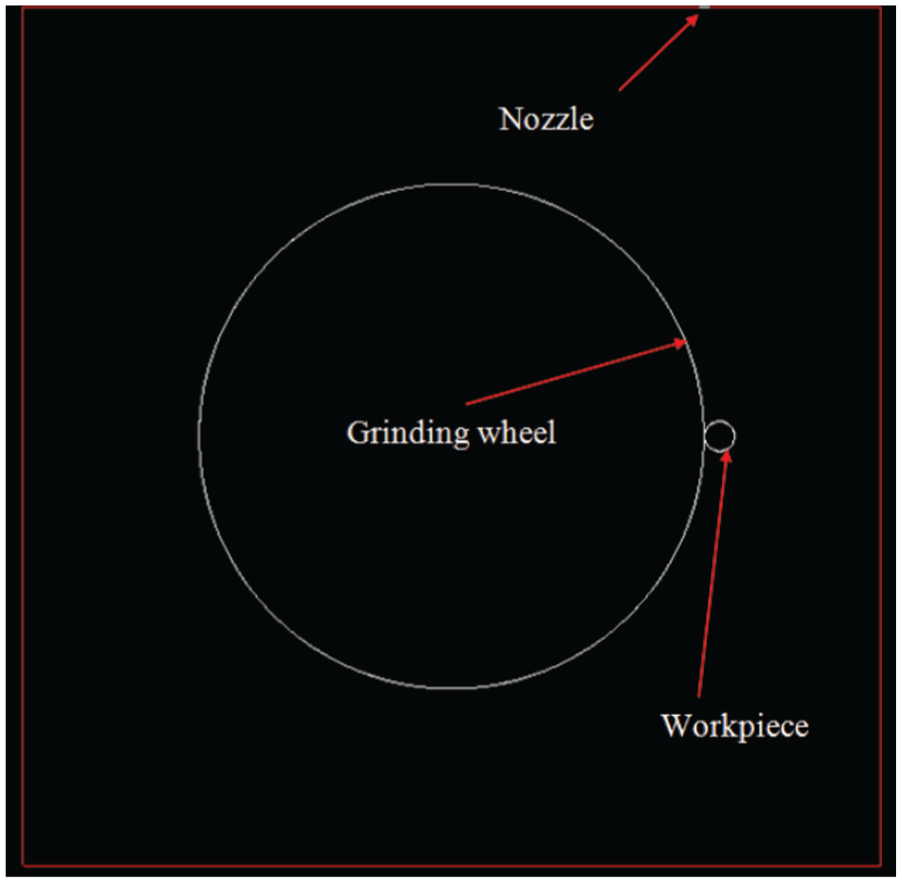
Geometry of the 2D numerical model.

The grinding wheel and the workpiece were modeled as solids with heat conduction as the main physical property. Volumetric heat generation (arising from the grinding thermal effects), solid zone motion (due to the grinding kinematics) and convection between the fluid and solid zones were included in order to represent an all-inclusive energy-transfer phenomenon in the computational domain. In order to accurately compute the heat transfer between the solid and the fluid, the grinding wheel was specified as a rough wall, since the roughness affects flow resistance as well as heat and mass transfer on the walls. The wall roughness here was specified with roughness that corresponds to the grain size. The grinding zone model hence includes pores and grains, that is, a homogeneous porous zone with permeability and inertial loss coefficients calculated from the grain and pore size (the assumed wheel porosity is 40%). The grinding zone is modeled as a moving heat source, that is, via an MRF rotating with the wheel. The reasoning behind this is that the porosity of the wheel significantly influences the useful flow rate through the grinding zone.¹⁶ The nozzle design^17–19 and fluid-supply parameters (nozzle angle, nozzle height, nozzle outlet area and fluid jet velocity),^20,21 however, were not the focus of modeling and analysis.

The computational grid is built of tetragonal elements and contains 54,828 cells, 110,600 faces and 55,773 nodes. A more detailed representation of the grinding zone grid structure is shown in Figure 2.

Figure 2.

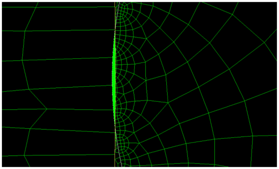
Detailed representation of the grinding zone computational grid.

The inclusion of the two-phase VOF model, the MRF and the RSM into the simulation represents a state-of-the-art approach to numerical modeling of fluid flow and thermal aspects in grinding. The advantages of this approach are as follows:

A wide range of length and time scales

Stationary and moving wall boundaries

Porous regions

An accounting for complex geometries, particularly in the contact region

Modeling rationale

VOF multiphase model

In order to accurately track the motion of the grinding fluid in and around the grinding zone to capture the correct multiphase flow dynamics, the VOF multiphase model was used along with a high-resolution interface-capturing numerical discretization scheme. The VOF multiphase model is a form of surface-tracking technique that is applied to a fixed Eulerian grid. In this model, there is a single set of momentum equations which is shared by all the fluids. The volume fraction of every fluid in each computational cell is tracked over the entire domain. The effect of surface tension along the interface between each pair of phases was implemented in the model. The model was them improved by specifying the contact angles between the phases and the walls. For example, a wall adhesion angle—in conjunction with the surface tension model—was specified in order to capture the effect of fluid adhesion on the solid walls, that is, the grinding wheel and the workpiece.

MRF

The relative motion between the grinding wheel and the workpiece (grinding kinematics) was captured by using the MRF for simulating time-averaged flow fields. The rotating domains were specified as three rotational reference frames: (1) around the workpiece, (2) around the grinding wheel and (3) around the porous grinding zone. In the model’s MRF steady-state approximation, individual cell zones can be assigned with different rotational and/or translational speeds. The flow in each moving cell zone is hence solved using the MRF equations. At the interfaces between the cell zones, a local reference frame transformation is performed to enable flow variables in one zone to be used to calculate flows at the boundary of the adjacent zone.

RSM

In turbulent fluid flows, the problem of modeling the Reynolds stress arises. For such turbulence closure modeling, the Boussinesq hypothesis is commonly used. The greatest disadvantage of this hypothesis is that turbulent dynamic viscosity is assumed to be an isotropic scalar quantity, which is not completely true. An alternative RSM approach is to solve the flow-transport equations for every term in the Reynolds stress tensor. It requires additional scale-determining equations (normally for turbulent dissipation rate): that is, five transport equations must be solved in 2D flows and seven in 3D flows. The RSM is clearly superior for fluid flows in grinding, where the anisotropic effect of turbulence has a dominant influence on the mean flow. The RSM includes the effects of streamline curvature, swirl, rotation and rapid changes in strain rate in a more precise way compared to one-equation and two-equation models. Therefore, it has higher ability to accurately model complex fluid flows and is used in this work.

Simulation

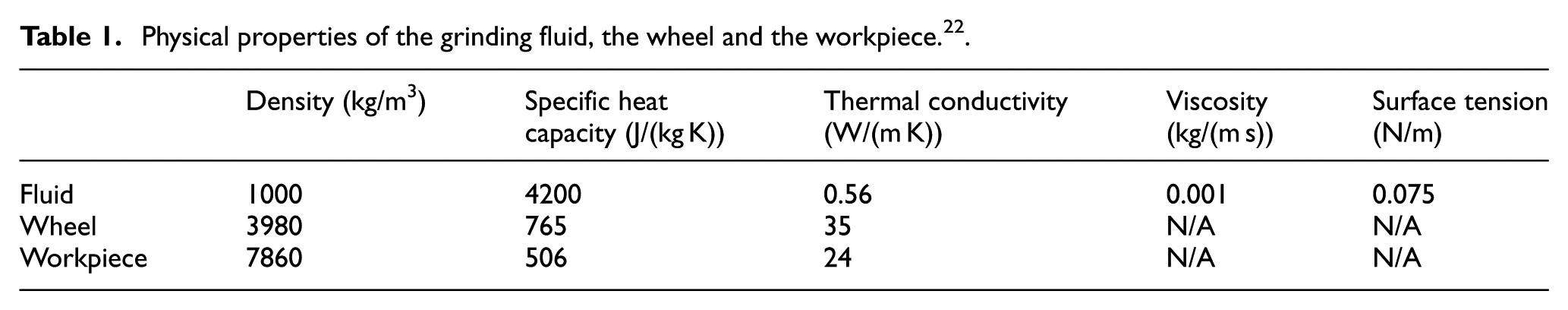
The grinding fluid used in the simulation was a water-based coolant (5% emulsion). The wheel used in the simulation was aluminum oxide with a grain size of 0.19 mm (value used for calculating the porosity parameters of the grinding zone). The workpiece material was HSS. The physical properties of the grinding fluid, as well as the two solids in the grinding zone, are given in Table 1.

Table 1.

Physical properties of the grinding fluid, the wheel and the workpiece.²²

	Density (kg/m³)	Specific heat capacity (J/(kg K))	Thermal conductivity (W/(m K))	Viscosity (kg/(m s))	Surface tension (N/m)
Fluid	1000	4200	0.56	0.001	0.075
Wheel	3980	765	35	N/A	N/A
Workpiece	7860	506	24	N/A	N/A

Four different grinding scenarios are considered in setting up the simulation:

Burned workpiece—ground without the use of grinding fluid (dry)

Burned workpiece—ground with the use of grinding fluid (cooling)

Unburned workpiece—ground without the use of grinding fluid (dry)

Unburned workpiece—ground with the use of grinding fluid (cooling)

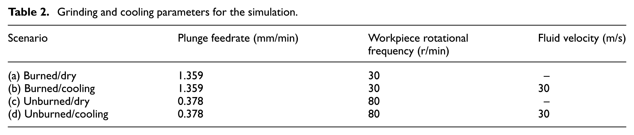
The grinding and cooling parameters associated with the four scenarios are given in Table 2. The wheel and workpiece diameters were 440 mm and 25 mm, respectively. The wheel speed was set constant at 63 m/s. Cooling considered the nozzle orifice diameter of 10 mm, the turbulence intensity of 3% and the turbulent length scale of 0.7 mm.

Table 2.

Grinding and cooling parameters for the simulation.

Scenario	Plunge feedrate (mm/min)	Workpiece rotational frequency (r/min)	Fluid velocity (m/s)
(a) Burned/dry	1.359	30	–
(b) Burned/cooling	1.359	30	30
(c) Unburned/dry	0.378	80	–
(d) Unburned/cooling	0.378	80	30

Simulation of the useful flow rate through the grinding zone

The grinding fluid enters the domain of the simulation from a nozzle at the top right corner of the domain boundary, as shown in Figure 3. This is a low-pressure injection of the grinding fluid (flood application). The fluid hits the grinding zone between the grinding wheel and the workpiece, where it is entrained by the rotating porous wheel, accelerated through the grinding zone and then expelled with the speed matching the wheel speed. Part of the applied fluid is deflected and sprayed to the sides due to the air barrier surrounding the grinding wheel, whereas some of the grinding fluid adheres to the wheel, but it is gradually released due to the centrifugal force. Adhesion of the grinding fluid to the solid surfaces depends on the wheel porosity and is included in the simulation by adding the surface tension effects via the VOF model.

Figure 3.

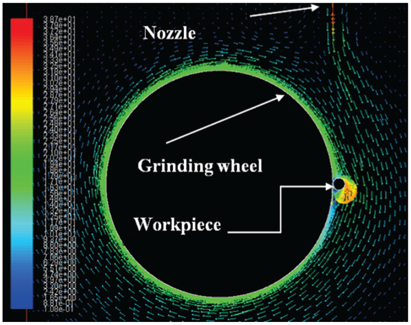
Fluid velocity vectors.

The useful flow rate is the fraction of the total fluid that actually enters the porous grinding zone. It can be directly measured (as percent utilization) experimentally by capturing the fluid at the exit from the grinding contact,²³ which requires a huge effort but can be carried out in a laboratory setting.

In our case, the simulation was used as an alternative to investigate the effects of the fluid and the wheel velocities on the useful flow rate. In order to facilitate the fluid flow analysis, the fluid motion is numerically characterized by fluid velocity vectors, along with their magnitude in meters/second. Some of the highest fluid velocities (around 39 m/s) are also found in the grinding zone, as shown in Figure 3. The increase in fluid velocity in the grinding zone is 30% compared to the velocity at the inlet.

The obtained results for the set cooling scenarios show that the useful flow rate is around 20%, on average, which agrees well with the reported experimental values of 5%–30%.²³

Simulation of the grinding temperatures

Thermal analyses of grinding, based on the moving heat source theory,²⁴ neglect the influence of the grinding fluid on the grinding temperatures. One of the exceptions is the research presented by Des Ruisseaux and Zerkle,²⁵ who considered the effect of cooling. In practice, however, almost all grinding operations are performed using some sort of cooling. To demonstrate the effects of cooling (and its efficiency), the simulations also include the dry grinding scenarios ((a) and (c) in Table 2).

A comparison of the temperature fields in the workpiece for cases of burned (b in Table 2) and unburned (d in Table 2) workpieces—with grinding fluid application—is shown in Figure 4. It can be seen that the temperature field (temperatures are given in °C) distorts in the direction of workpiece rotation due to the cooling of the bulk material by the grinding fluid and surrounding air. The shape of the temperature field is the same in both cases, but the temperature values are higher in the points of comparison, in the case of the burned workpiece.

Figure 4.

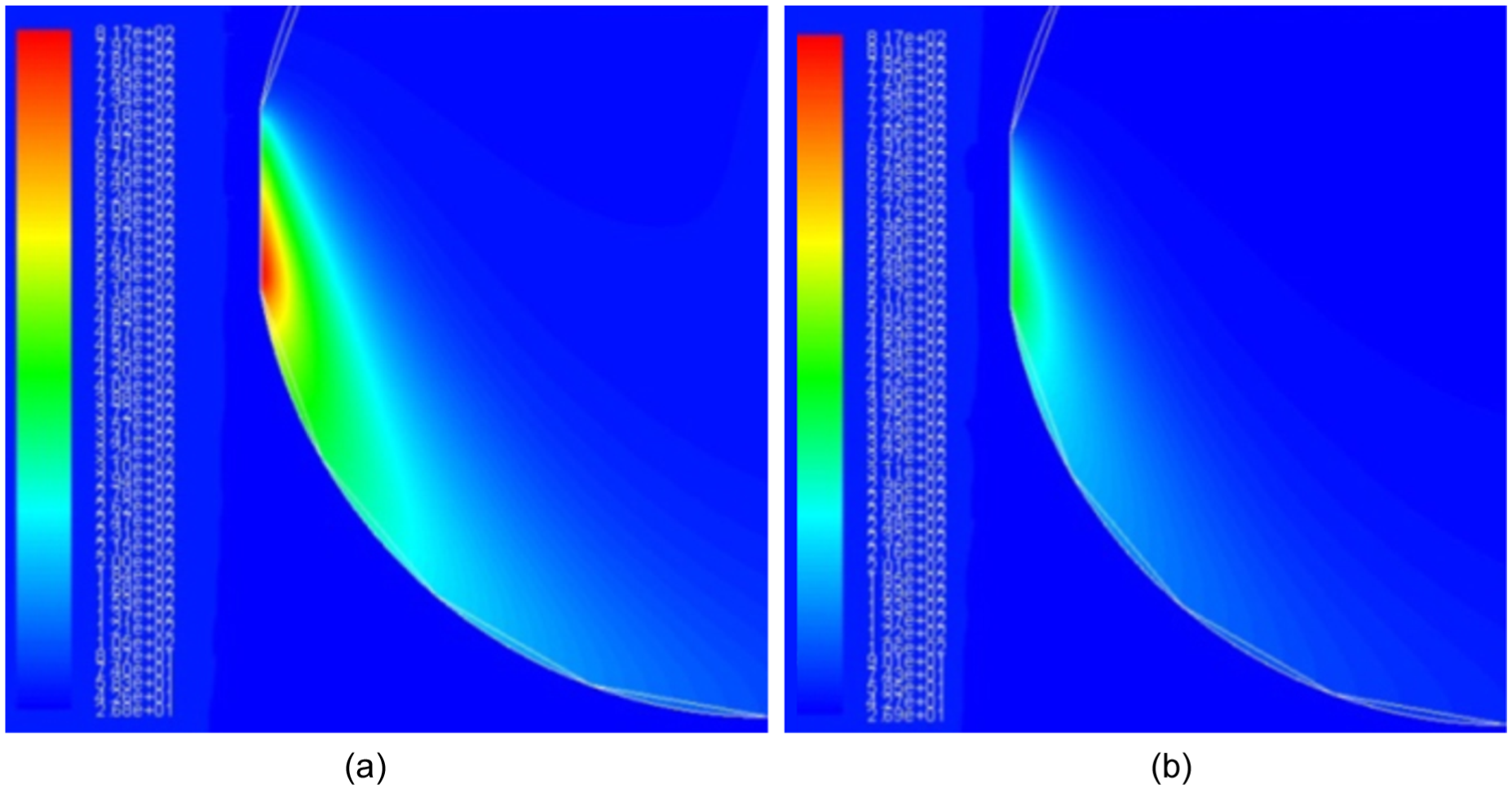
Grinding temperatures in (b) burned and (d) unburned workpieces.

From the simulations, it is possible to ascertain that a grinding fluid provides a bulk cooling of the workpiece, reducing the workpiece surface temperatures of the burned workpiece by 26% (and by 28% on the surface of the unburned sample), thus helping to reduce the thermal loads. Figures 5 and 6 show the temperatures for the burned and unburned workpieces, with and without application of grinding fluid. The temperatures are shown for a non-dimensional parameter x/l_c , describing the relative position in the grinding zone, where l_c is the contact length.

Figure 5.

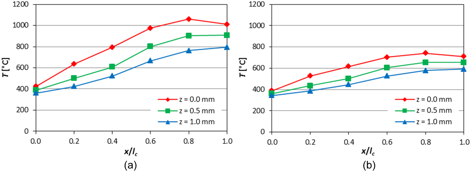
Temperatures in burned workpiece: (a) without and (b) with grinding fluid application.

Figure 6.

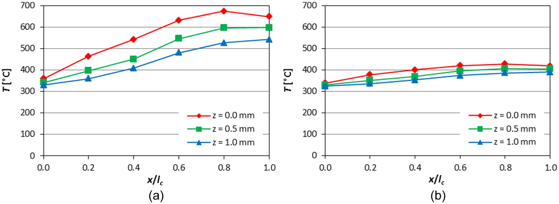
Temperatures in unburned workpiece: (c) without and (d) with grinding fluid application.

Based on the simulations above, it is further possible to quantify the effectiveness of cooling for the burned and unburned workpieces. The predictions suggest that the maximum workpiece surface temperatures can be reduced by 30%–40% when applying the grinding fluid as compared to dry grinding. This means that cooling by grinding fluids at the grinding zone is not totally ineffective for this type of operation.⁴ This is further validated by the simulated grinding energy fractions, as shown in Table 3.

Table 3.

Simulated energy partition (energy into the workpiece) and energy into the fluid.

Scenario	Energy into the workpiece (%)	Energy into the fluid (%)
(a) Burned/dry	82.2	0.0
(b) Burned/cooling	75.1	9.6
(c) Unburned/dry	80.5	0.0
(d) Unburned/cooling	72.8	10.2

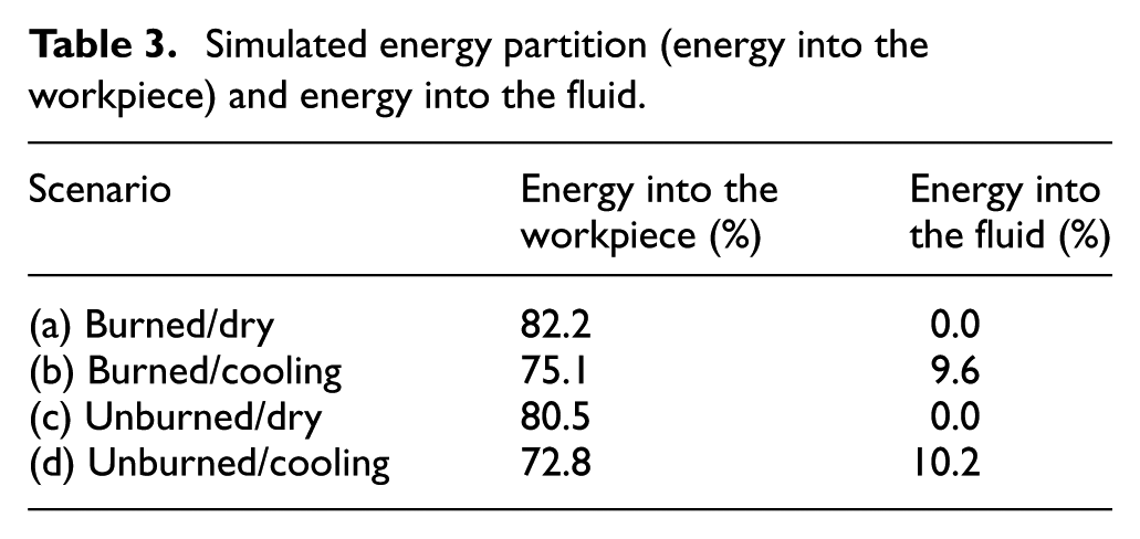
The results are again in good agreement with previous estimates; Malkin and Guo⁴ reported that for shallow-cut grinding with conventional abrasive wheels, the energy partition is typically 60%–85%. The cooling reduces the energy partition by about 10% when compared to dry grinding, which is low but not negligible. This is corresponding to the fraction of the total grinding energy convected by the grinding fluid - about 10% for the simulated cases. Heat convection by the grinding fluid could be increased, leading to larger fraction of the total grinding energy. Effective fluid delivery is therefore essential for improving the thermal aspects of grinding.

Experimental

The experiments were carried out on a standard computer numerical control (CNC) cylindrical grinding machine. The workpieces (diameter = 25 mm) were made of AISI M2 HSS with the following chemical composition: C: 0.9%, Cr: 4.2%, Mo: 5%, W: 6.4% and V: 1.8%. The hardness of the workpiece surface was 64 HRC obtained by the following heat treatment: hardening in a protective atmosphere at 1180 °C and two temperings at 560 °C (with at least 1 h holding time). An 80-grain mesh, J-grade, seven-structure, vitrified-bonded, aluminum oxide wheel was used (diameter = 440 mm, width = 35 mm). The wheel was dressed prior to each experimental trial with a diamond blade (width = 0.35 mm) using dressing depth = 0.01 mm and traverse dressing feed rate = 300 mm/min. The width of grinding was held constant for all the experiments and set to 29 mm (not using the full wheel width). An emulsion in 5% concentration was used, as considered in the simulation. Dry grinding tests were not run due to potential damage to the machine.

Two sets of cylindrical grinding experiments were carried out to produce the burned (scenario (b)) and the unburned workpieces (scenario (d)). The experiments included changing the plunge feedrate and the workpiece rotational frequency according to Table 2. This gives two distinct grinding conditions (Table 4) that generate the grinding temperatures leading to burned and unburned workpieces.

Table 4.

Grinding conditions.

Workpiece	Equiv. depth (µm)	Chip thickness (µm)	Contact length (mm)	Spec. MRR (mm³/(mm s))
Burned	45.29	1.246	1.04	1.78
Unburned	4.73	1.156	0.34	0.50

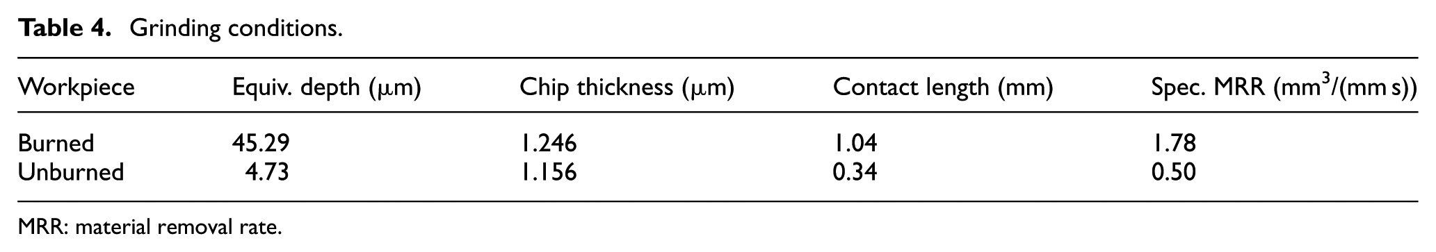
MRR: material removal rate.

Stress profiles were measured on the ground surfaces, comparing burned with non-damaged surface. This has been performed using an X-ray diffractometer (Figure 7) featuring the Cr K alpha X-ray source to acquire the diffraction peak at a Bragg angle 2θ = 156.4°, using collimator size of 2 mm in diameter. Modified Sin²ψ method measurements were performed at four ±ψ = 45° angles with no additional oscillations and 7 s explosion time. The Young’s modulus and Poisson’s ratio used for the reflection were 211 MPa and 0.3, respectively.

Figure 7.

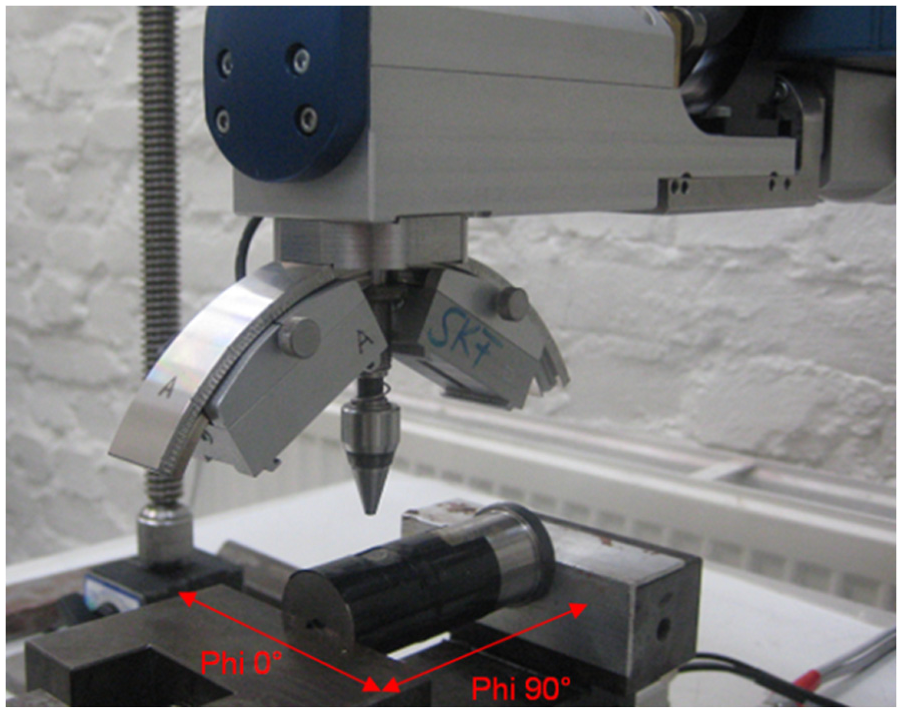
X-ray diffractometer setup.

The residual stresses versus depth profiles were measured by removing successive layers of material up to the depth of 500 µm by electro-polishing, thus avoiding the reintroduction of additional residual stresses. Considering the size of the workpiece in relation to the stressed layer (<200 µm), the difference between the redistributed stress due to layer removal and the true stress state (relaxation effect) is negligible. Therefore, no corrections were made for layer removal.

Surface integrity and simulation assessment

The grinding temperatures affect the surface integrity of ground workpieces; therefore, the assessment of surface integrity, based on analyzing the residual stress, heat-affected zone depth and full width at half maximum (FWHM) profile, provides a good method to verify the simulated grinding temperatures. Surface integrity indicators are hence used for indirect verification of the simulation.

Stresses in the circumferential direction (phi 0°), phi 45° direction and axial direction (phi 90°) were evaluated. The subsurface residual stresses differ slightly between the circumferential and axial directions. This is evident especially in the case of the burned workpiece (Figure 8(a)). On the surface, this difference is less expressed. Residual stresses are predominantly compressive on the surface, and they increase monotonically with the depth. In the burned workpiece, residual stress amplitudes shift from compressive to tensile approximately 10 µm beneath the surface, while the maximum tensile magnitude of 1400 MPa is observed at about 50 µm below the surface. Such high values of tensile residual stresses are typically caused by high thermal loads, for example, temperatures between 600 and 800 °C that are predicted by the simulation as shown in Figure 5(b). In contrast, the surface integrity of the unburned workpiece is improved, which is evident from a significantly lower tensile residual stresses—reaching the maximum of 100 MPa 10 µm beneath the surface as shown in Figure 8(b). This profile indicates low grinding temperatures in the 300–400 °C range, which yield an unburned workpiece thus confirming the simulated temperatures shown in Figure 6(b). A closer look at the residual stress profile for the unburned workpiece also reveals that the most compressive stresses (−200 MPa) are reached in circumferential direction, while the minimal are observed in axial direction (−40 MPa).

Figure 8.

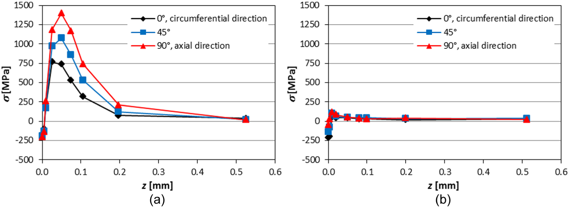
Residual stress in (b) burned and (d) unburned workpieces.

The assessed heat-affected zone depths tend to further verify the simulation. In case of the burned workpiece, the heat-affected zone reaches a depth of 250 µm, while this depth is only 20 µm for the unburned workpiece. The latter depth is significantly lower, meaning that practically no tensile residual stress is present in case of unburned workpiece.

In addition to residual stress profiles, FWHM profiles also give further insight into stresses, hardness and plastic deformation. For example, FWHM values typically increase with increasing hardness and vice versa. The FWHM profiles shown in Figure 9 consist of the average values from psi angles, where the untreated material values are approximately 6°. The surface integrity assessment is particularly interesting for the workpiece surface. The FWHM profile of the unburned workpiece surface is monotonous, meaning that the surface hardness is not reduced. The grinding temperatures here are below the tempering temperature of 560 °C, which agrees with the simulation. On the other hand, however, the FWHM values rapidly increase at the burned surface, reaching the maximum of 8.5°. This indicates a severe plastic deformation from the strain-hardening effect caused at high grinding temperatures. Such an increase in FWHM from its initial value points to a decreased hardness (overtempering) and significant onset of residual tensile stresses. The grinding temperatures causing this increase are therefore certainly higher than the tempering temperature (560 °C), which again is in good agreement with the simulation.

Figure 9.

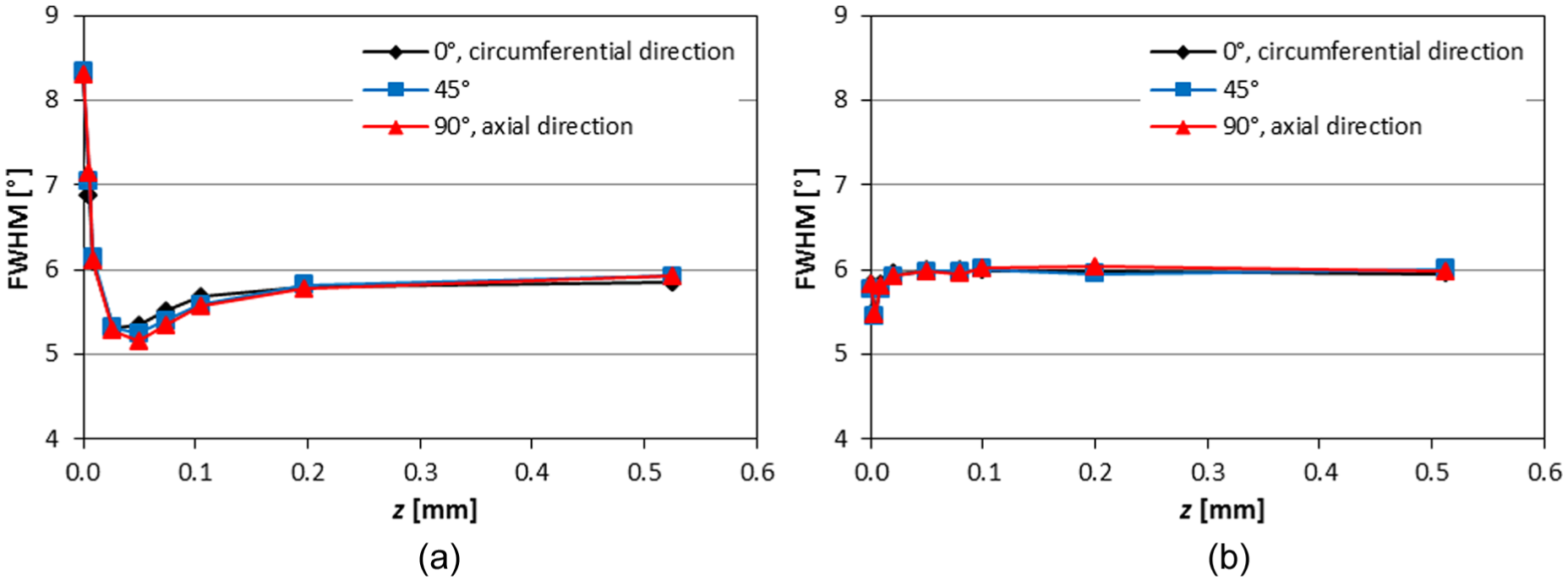
FWHM profiles in (b) burned and (d) unburned workpieces.

Conclusion

A novel analysis of thermal and fluid flow aspects in grinding is described. The analysis uses numerical modeling through CFD. The results indicate that the useful flow rate, is around 20%. Application of the grinding fluid provides bulk cooling of the workpiece. It was found that cooling in shallow-cut grinding operations using conventional abrasive wheels is not insignificant, since the workpiece surface temperatures can be reduced by 30%–40% when compared to dry grinding. The fraction of the energy convected by the grinding fluid is about 10%. The obtained energy partitions (about 70–80%) are in good agreement with previous estimates. CFD results indicate an adequate match between the simulated grinding temperatures and surface integrity measurements. In the burned workpiece, residual stresses are tensile, caused by temperatures ranging between 600 and 800 °C. Undesired tensile residual stresses are avoided when the grinding temperatures stay in the 300–400 °C range. In the latter case, the heat-affected zone is minimal (20 µm) and with very low tensile stress levels where the overtempering of the workpiece material is avoided, as implied by the corresponding FWHM profile.

Footnotes

Declaration of conflicting interests

The author(s) declared no potential conflicts of interest with respect to the research, authorship and/or publication of this article.

Funding

The author(s) received no financial support for the research, authorship, and/or publication of this article.

References

Badger

Grindability of conventionally produced and powder-metallurgy high-speed steel. CIRP Ann: Manuf Techn 2007; 56: 353–356.

Krajnik

Drazumeric

Badger

et al . Particularities of grinding high speed steel punching tools. Adv Mat Res 2011; 325: 177–182.

Chen

Rowe

McCormack

DF.

Analysis of the transitional temperature for tensile residual stress in grinding. J Mater Process Tech 2000; 107: 216–221.

Malkin

Guo

Thermal analysis of grinding. CIRP Ann: Manuf Techn 2007; 56: 760–782.

Drazumeric

Badger

Krajnik

Geometric, kinematical and thermal analyses of non-round cylindrical grinding. J Mater Process Tech 2014; 214: 818–827.

Malkin

Anderson

RB.

Thermal aspects of grinding: part 1—energy partition. J Eng Ind: T ASME 1974; 96: 1177–1183.

Liao

Luo

Yang

TH.

A thermal model of the wet grinding process. J Mater Process Tech 2000; 101: 137–145.

Mamalis

Manolakos

Markopoulos

et al . Thermal modelling of surface grinding using implicit finite element techniques. Int J Adv Manuf Tech 2003; 21: 929–934.

Mao

Zhou

Ren

et al . Analysis and FEM simulation of temperature field in wet surface grinding. Mater Manuf Process 2010; 25: 399–406.

10.

Klocke

Duscha

Linke

et al . FEM-based simulation of temperature in speed stroke grinding with 3D transient moving heat sources. Adv Mat Res 2011; 223: 733–742.

11.

Chang

CC.

An application of lubrication theory to predict useful flow rate of grinding fluids on grinding porous media. Tribol Int 1997; 30: 575–581.

12.

Ebbrell

Wooley

Tridimas

et al . The effects of cutting fluid application methods on the grinding process. Int J Mach Tool Manu 2000; 40: 209–223.

13.

Gviniashvili

Woolley

Rowe

WB.

Useful grinding fluid flow rate in grinding. Int J Mach Tool Manu 2004; 44: 629–636.

14.

Morgan

Jackson

et al . Optimisation of fluid application in grinding. CIRP Ann: Manuf Techn 2008; 57: 363–366.

15.

Baines-Jones

Nozzle design for improved useful fluid flow in grinding. PhD Thesis, Liverpool John Moores University, Liverpool, 2010.

16.

Guo

Malkin

Analysis of fluid flow through the grinding zone. J Eng Ind: T ASME 1992; 114: 427–434.

17.

Alberdi

Sanchez

Pombo

et al . Strategies for optimal use of fluids in grinding. Int J Mach Tool Manu 2011; 51: 491–499.

18.

Lopez-Arraiza

Castillo

Dhakal

et al . High performance composite nozzle for the improvement of cooling in grinding machine tools. Compos Part B: Eng 2013; 54: 313–318.

19.

Rouly

Bauer

Warkentin

An investigation into the effect of nozzle shape and jet pressure in profile creepfeed grinding. Proc IMechE, Part B: J Engineering Manufacture. Epub ahead of print 22 May 2015. DOI: 10.1177/0954405415584960.

20.

Heinzel

Meyer

Kolkwitz

et al . Advanced approach for a demand-oriented fluid supply in grinding. CIRP Ann: Manuf Techn. Epub ahead of print 23 April 2015. DOI: 10.1016/j.cirp.2015.04.009.

21.

Parthasarathy

Malkin

Effect of fluid application conditions on grinding behaviour. Proc IMechE, Part B: J Engineering Manufacture 2010; 224: 225–235.

22.

Zhang

Rowe

Morgan

MN.

An improved fluid convection solution in conventional grinding. Proc IMechE, Part B: J Engineering Manufacture 2013; 227: 832–838.

23.

Engineer

Guo

Malkin

Experimental measurement of fluid flow through the grinding zone. J Eng Ind: T ASME 1992; 114: 61–66.

24.

Jaeger

JC.

Moving sources of heat and the temperature at sliding contacts. J Proc Roy Soc New S Wales 1942; 76: 203–224.

25.

Des Ruisseaux

Zerkle

. Thermal analysis of the grinding process. J Eng Ind: T ASME 1970; 92: 428–434.

The use of computational fluid dynamics in the analysis of fluid flow and thermal aspects in grinding

Abstract

Keywords

Introduction

Background

Numerical model

Description of the model

Modeling rationale

VOF multiphase model

MRF

RSM

Simulation

Simulation of the useful flow rate through the grinding zone

Simulation of the grinding temperatures

Experimental

Surface integrity and simulation assessment

Conclusion

Footnotes

Declaration of conflicting interests

Funding

References