
Abstract
Flow boiling in microchannels has been researched for decades due to its potential for heat transfer applications in micro structured devices. The large number of existing experimental datasets and fitted correlations show considerable scatter and lack a mechanistic basis. The computational fluid dynamics (CFD) model developed here applies to boiling in the annular flow regime and provides insights into the underlying behaviour. Analysis of the heat transfer augmentation by interfacial waves is studied. Parametric investigations are performed using the model to understand the impact of important flow and system parameters. The calculated heat transfer coefficients are consistent with those from existing correlations, showing no more scatter than the data used to create them.
Introduction
Development and application of micro structured devices in modern science and engineering technologies have brought major challenges for heat transfer in microchannels. 1 Flow boiling has received increasing interest due to its potential for addressing the thermal management challenges arising from the increasing heat flux density in micro structured devices. 2 However, the vast number of experimental and analytical studies of microchannel flow boiling conducted by many researchers in the past few decades show contradictory results. Computational fluid dynamics (CFD) approach has been used for microchannel flow boiling research in recent years, but little CFD work focuses on annular flow, which is the prevalent flow regime. This paper proposes a CFD model for the detailed study of annular flow boiling in microchannels. Verification of the CFD heat transfer model is presented and detailed analysis of the annular flow boiling mechanism is performed. Studies of the effects of some important flow and geometric parameters are also performed and discussed.
Literature review
Comprehensive reviews of microchannel flow boiling are available in Thome, 3 Garimella and Sobhan, 4 Bertsch et al., 5 Kandlikar 2 and Baldassari and Marengo, 6 where many datasets from experimental studies are compared with the available correlations and theoretical models. However, not only do the experimental results show contradictory outcomes, but also the correlations do not provide satisfactory predictions. Experiments showed that the two-phase flow regime in microchannels transitions from bubbly to slug, slug-annular and annular flow at very low vapour qualities (x < 0.1). 7 Data from Lee and Mudawar 8 show that heat transfer is still strong in the annular regime (x > 0.1), where very few bubbles are observed and the heat transfer coefficient does not decrease much compared with that in the bubbly region. Particularly, data from Bertsch et al., 9 Lin et al. 10 and Yun et al. 11 yield the peak heat transfer coefficients at vapour qualities in the range 0.1–0.6, in which the two-phase flow regime is annular.
Apart from the experimental and analytical studies, flow boiling has also been studied numerically using different approaches. Guo et al. 12 reviewed the CFD work on microchannel flow boiling and presented the main numerical approaches used for the analyses. However, most of the flow boiling simulations focus on bubble growth,13–15 bubble formation and the subsequent bubble dynamics,16–21 bubble merging 22 and liquid evaporation in Taylor bubbles.23,24 Only a few numerical studies of phase change in microchannel annular flow25–27 have been reported and these are mostly for condensation.
Da Riva and Del Col
25
performed a three-dimensional (3D), steady-state simulation of R134a condensation in a 75 mm long, 1 mm diameter circular microchannel using the commercial CFD solver Fluent 6.3. The grid spacing used in the core region was approximately 15 µm and was refined to 0.8 µm in the near wall region. An implicit volume of fluid (VOF) method
28
and a modified HRIC scheme
29
were used to model the multiphase interface. A modified k–ω turbulence model
30
was applied in the gas phase. The phase change mass source (S) was computed based on the normalised temperature difference between the interface temperature and a constant saturation temperature as
Chen et al.
26
used Fluent 6.1 to perform a three-dimensional transient condensation simulation of FC-72 in a 300 mm long microchannel with 1 mm2 cross section. The computational domain contained around 200,000 cells, but the details of the grids in each spatial direction are not provided. However, it is estimated from the geometry and the cell number that the number of grids across the side length is less than 10. According to the analysis of Gupta et al.
32
which showed that at least five cells are needed to resolve a thin liquid film in microchannel slug flow, the mesh used in Chen et al.
26
is clearly too coarse to perform accurate microchannel slug, transition and annular flow simulations. The VOF method was used to capture the interface and a second-order implicit method is used for temporal discretisation. A k–ɛ model
33
was used to model turbulence. The interphase mass transfer was calculated using
A quasi-3D numerical approach for the simulation of annular flow evaporation in rectangular microchannels is proposed by Jesseela and Sobhan. 27 The numerical approach used solves the equations on a cross section and then marches in the flow direction to obtain a 3D solution. In their work, annular flow phase change was modelled in a 15 mm long channel with a rectangular cross section. The edge lengths of the rectangular cross section vary from 30 µm to 300 µm. The mesh size in the cross-sectional domain was 41 × 81. It was assumed that the flow was laminar, incompressible and steady, for both the liquid and the vapour phases. Subcooled water enters at the inlet and then the phase change is calculated based on the heat input assuming that no superheating occurs in the gas and liquid phases. The numerical results were shown to be in agreement with the experimental data of Qu and Mudawar 34 for the pressure drop along the flow direction. The results for the effect of vapour quality on heat transfer qualitatively match the observation by Ong and Thome 35 for refrigerant flow. Although this approach provides some qualitative predictions of annular flow boiling, the assumption of steady annular flow is not universally valid. Furthermore, the assumption that all the input heat is used to evaporate liquid neglects the dynamics of the mass transfer at the phase interface.
The above review shows that despite the importance of annular flow boiling in microchannels, there is a complete lack of detailed numerical studies in this area. In our previous work, 36 a numerical model for isothermal annular flow was proposed and validated. In this paper, a phase change model is added to form a complete model for annular flow boiling.
Mathematical modelling
The Eulerian-based multiphase flow model used previously 36 is extended to include thermal and phase change models.
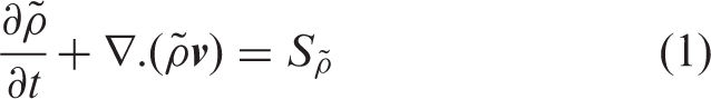
Governing equations
The governing equations (1) to (3) are based on the following assumptions:
All the fluids are Newtonian and incompressible. Homogeneous velocities and temperatures are assumed, i.e. when the two fluids coexist they have the same velocity and temperature. The gravitational/buoyancy force is neglected. Viscous dissipation is neglected. The flow is laminar, with velocities low enough to permit the use of a thermal energy, as opposed to a total energy, equation.
Continuity
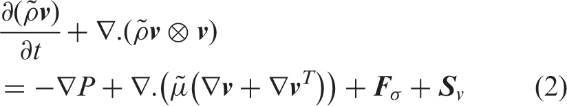
Momentum
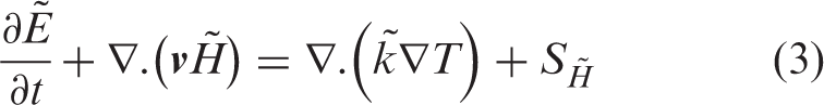
Energy
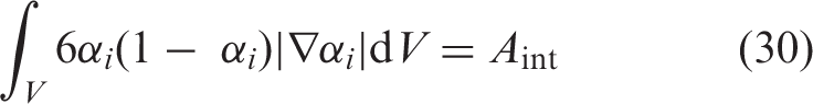
Additionally, a transport equation for a colour fraction is solved to identify the interface location and to calculate the volume fractions
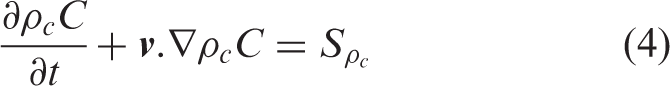
The volume fraction for one fluid is obtained using equation (4) and the other is obtained from


The continuum surface force (CSF) model of Brackbill et al.
37
is used for surface tension modelling. In this model, the surface tension force is calculated via

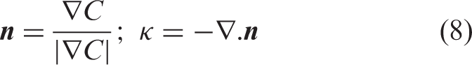
The objective of this implementation is to replace the curvature calculation method of the original CSF method with a height function algorithm which yields more accurate curvature values than equation (8). The detailed development and implementation of the height function method into ANSYS Fluent is presented in Guo et al. 38
Note that the bulk mass, momentum and energy sources in equations (1) to (3) are zero as conservation of mass, momentum and energy needs to be maintained during the phase change processes. However, local sources may become non-zero due to the numerical smoothing procedure used in their solution, described in the source terms used in the modelling of the phase change process section.
Phase change model
The phase change model implemented in the simulations is used to calculate the local interphase mass flux, depending on the local conditions at the liquid–gas interface. In the current simulations, the Tanasawa model39 is modified for the flow boiling process, as shown in equation (9)
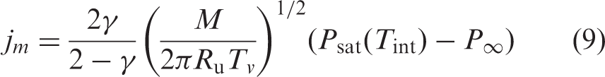

For boiling at an interface, the mass flux depends on the difference between the saturation pressure evaluated using the interface temperature and the local gas phase pressure. However, in any numerical simulation using a VOF method, the interface is smeared, so that the boiling source must be applied across a number of computational cells. It is straightforward to evaluate the saturation pressure in each cell but it is not so clear how to choose a local pressure, as the gas phase pressure is modified by surface tension effects inside the liquid region. There is only a small pressure drop along the flow direction (<1.3 kPa in the current simulations) which is small compared with the system pressure. Therefore, it was decided to use the constant system pressure
Boundary conditions
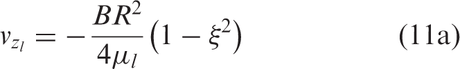
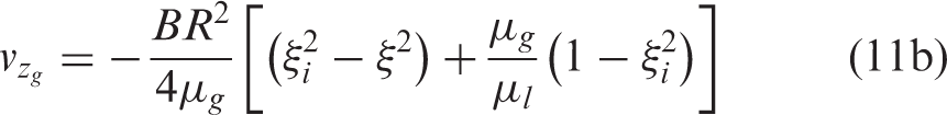
The inlet velocity profiles are obtained from the analytical solution of Fouilland et al.
43
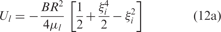
In order to analyse how interfacial instabilities affect flow boiling, various interface perturbation approaches can be used. For the current work, the time-dependent interface location at the inlet is perturbed as in Guo et al.
36
via

Once the perturbed interface location is calculated using equation (13), the velocity profiles at the inlet boundary depend on time and cannot be specified using equations (12a) and (12b) which provides two constraints on the three remaining variables (Ul, Ug, and B). To achieve a closed solution, either the liquid superficial velocity (“fixed Ul perturbation”) or the pressure gradient (“fixed B perturbation”) was fixed. The inlet fluid velocity profiles were then determined according to equations (11) and/or (12). Note that the inlet mean flow rates of the smooth and two perturbed cases presented later are not identical but the differences between them are typically less than 1%.
A zero average pressure boundary condition is used for the outlet, together with a damping treatment to maintain the interface at the outlet parallel to the flow axis, in order to avoid reversed flow. The detailed implementation of the outlet boundary condition and the modified damping model of Park et al. 44 are described in Guo et al. 36
For the inlet thermal boundary condition, the gas and liquid temperatures are set to the saturation temperature for the system pressure under consideration. A constant heat flux is applied at the channel wall.
Initial conditions
The velocity and volume fraction fields are initialised using equations (11) and (12). The temperature and pressure fields are initialised with the constant system pressure and the corresponding saturation temperature. As the heat applied at the wall conducts into the liquid, it becomes superheated and the evaporation mass flux in equation (9) becomes non-zero. However, evaporation only occurs in those cells for which there is a non-zero interfacial area, with the evaporation source being the product of the flux and interfacial area.
CFD methodology
The commercial software ANSYS Fluent (14.5 and 15.0.7) is used to model 2D, axisymmetric gas–liquid annular flow in a microchannel. The double precision transient solver is used.
The volume of fluid method
As noted previously, the VOF method is used to capture the interface between the liquid film and gas core. The explicit Piecewise-Linear Interface Calculation (PLIC) scheme developed by Youngs 45 is used to track the interface with sub-stepping to ensure the Courant number remains below 0.25. However, the actual time-step used for the simulations is smaller as it is limited by stability of the boiling source terms.
Source terms used in the modelling of the phase change process
To implement the phase change mass flux numerically, it must be transformed into a volumetric source. As noted above, this is done as follows:

As fluid is moved from the liquid to gas phase, it takes its momentum with it so that we have


The energy sources also need to be calculated depending on the direction of phase change. For evaporation, the energy sources are


A highly superheated interface will generate a high mass transfer rate which may cause numerical instabilities to occur. This is particularly so if a high evaporation flux is calculated in a cell that contains relatively little liquid. A numerical smoothing procedure proposed by Hardt and Wondra
46
used in their phase change simulations was implemented to improve the numerical stability by means of shifting such a source to the liquid side of the interface and smearing the mass source terms (
First, the boiling mass source term is shifted to the liquid side and the latent heat source is then calculated using the shifted mass source. This step is shown in equation (18) below


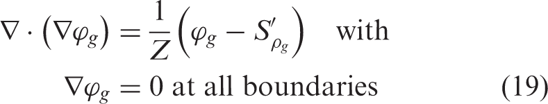
The second step of the procedure is smoothing of the mass source terms to avoid the generation of unphysical local velocities due to large source term, and the mass source term is smeared over a few cells near the interface, using the diffusion approach shown in equation (19) to generate the diffused mass source
An example of the original and the modified source terms is shown in Figure 1. The legends in the figure show that smoothed gas and liquid mass sources (
Typical original and modified phase change source terms in a boiling simulation: (a) original gas mass source; (b) shifted latent heat source; (c) diffused gas source; (d) final gas mass source; and (e) final liquid mass source. The solid black lines denote the gas–liquid interface.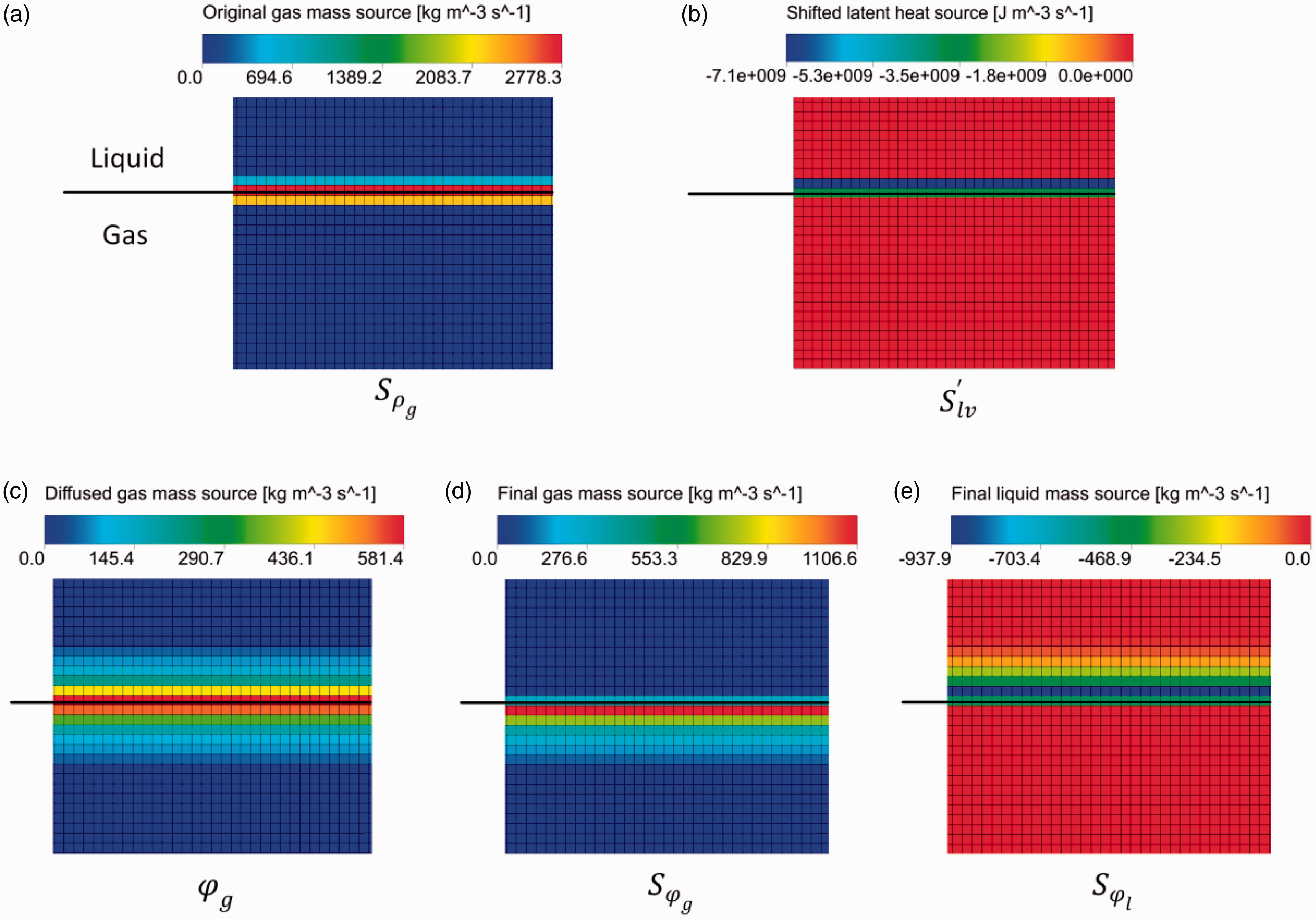
After the mass source terms are smoothed, the corresponding bulk mass, momentum and energy sources need to be calculated based on the smoothed mass source (


As the latent heat sources are calculated individually, the energy source now consists of the latent heat source and the enthalpies of the removed liquid and added gas

As shown in Figure 1, the final mass sources of the gas and liquid phases are diffused over several cells into each phase separately, so the bulk sources calculated using equation (20) may become locally non-zero. Therefore, the use of equations (20b) and (20c) is critical to prevent artificial acceleration/deceleration and heating/cooling. Global conservation is guaranteed as the smoothing procedure is performed under this constraint. However, as shown in Figures 1(d) and (e), the final gas and liquid sources are located in different cells which may have different local velocity and temperature values. Therefore, the summed momentum and energy sources calculated as volume integrals of the bulk source terms may become non-zero. However, the mass source is controlled to be smeared over only a few cells near the interface to minimise this effect in order to conserve momentum and energy during the phase change processes.
Coding and parallel considerations
The boundary and initial conditions, the outlet damping model, the height function method and the phase change model including the numerical smoothing procedure are coded in User-Defined Functions (UDFs) of ANSYS Fluent. The simulations are run in parallel on multiple computational nodes and parallelisation was ensured as described in Guo et al. 38 and the ANSYS Fluent 15.0 UDF Manual. 47
Numerical solver options
The SIMPLE algorithm of Patankar
48
is used for the pressure–velocity coupling. The implicit body force option is enabled to take into account the partial equilibrium of the pressure gradient and the body forces because the surface tension force is large compared with the viscous force (
Simulation results
The annular flow simulations are performed using circular channels of diameter D = 0.25 to 2 mm and length L = 10D to 50D. The 2D, axisymmetric computational domain is shown in Figure 2. The initial section of length LA is the region of interest where the phase change model is enabled. The final region of length LD serves as a numerical beach for wave damping to minimise any effect of the exit boundary conditions on the boiling zone. The two are separated by a short (∼D) adiabatic zone. The physical properties of water and steam are extracted from the NIST chemistry webbook.
49
Schematic representation of the computational domain.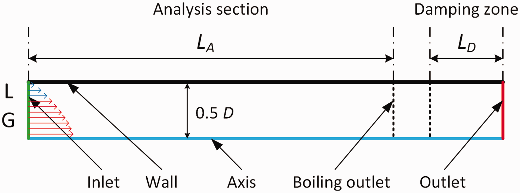
Grid-independence study
In our previous work, the dynamics of the interfacial waves in microchannel annular flow have been shown to be independent of grid spacing at Δ = D/200.
36
To perform the simulations with heat transfer and phase change, the mesh density needs to be checked with the energy equation and the phase change model enabled. An annular flow boiling simulation in a 1 mm diameter channel of L = 13D (LA = 10D and LD = 2D) at 101.3 kPa is used for this purpose. Liquid and gas superficial velocities of Ul = 0.11 ms−1 and Ug = 6 ms−1 are used to calculate the velocity profile for the inlet boundary and the initialisation. A fixed Ul perturbation of amplitude
The boiling simulation was firstly performed using four square meshes with grid spacing Δ = D/100 to Δ = D/300. To characterise the boiling process, the overall boiling mass source over the computational domain is calculated as
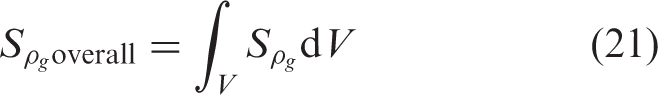
Figure 3 illustrates the overall vaporisation mass source as a function of the simulation time. It is clear from Figure 3 that when the mesh is refined, the calculated evaporation rate decreases until the mesh is refined to Δ = D/200 beyond which further refinement has no impact. Moreover, the simulations for the two low mesh resolution cases diverged shortly after t = 20 ms.
Overall vapour mass source obtained using various mesh densities.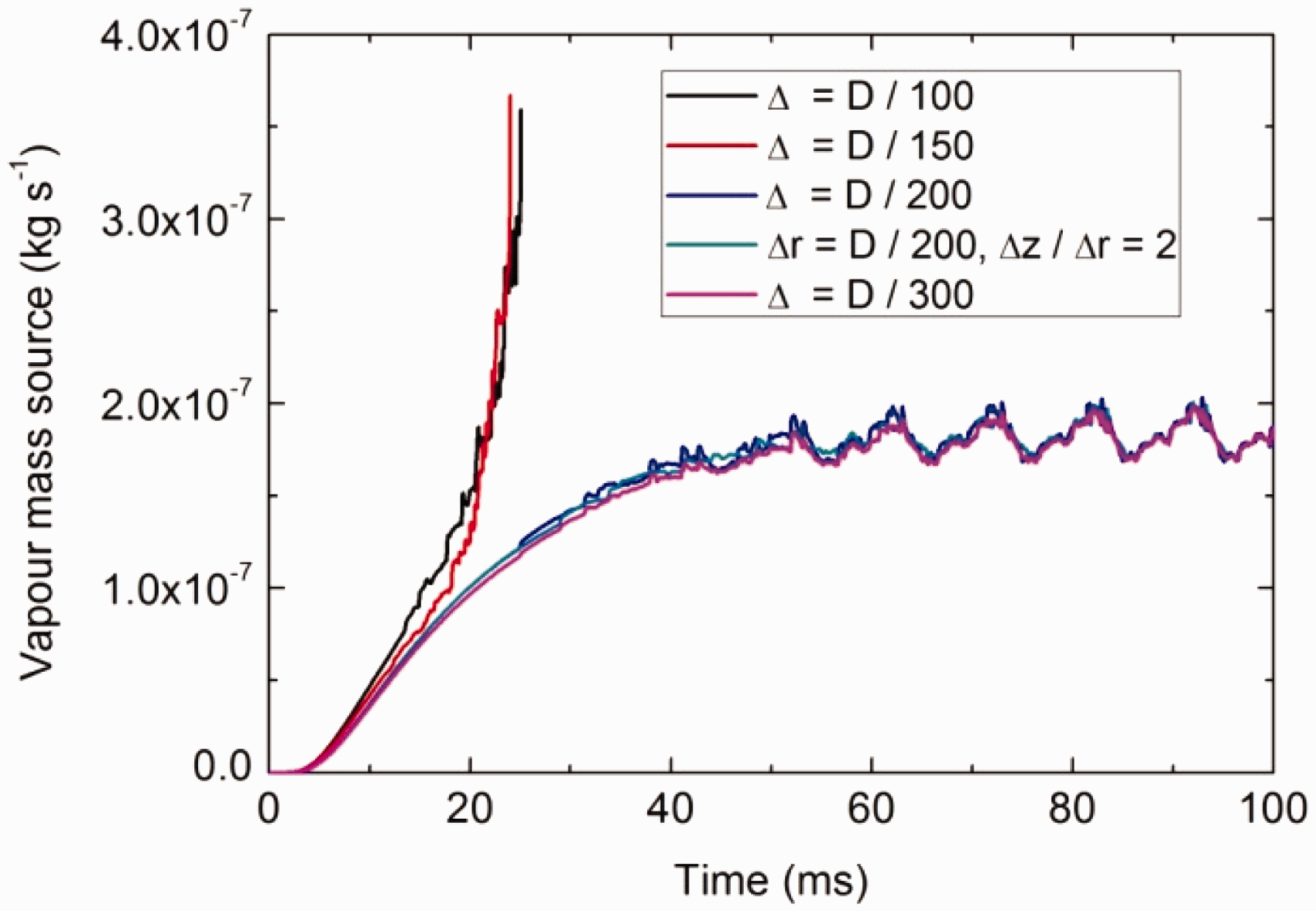
As shown in Figure 3, a rectangular mesh of aspect ratio
In the above simulations, a time-step of 5 × 10⁻⁷ s corresponds to a maximum Courant number of 0.10 for the grid spacing Δ = D/200. The time-step size for the Δ = D/200 case was increased from 5 × 10 − 7 s to 1 × 10⁻⁶ s and the results showed no difference. The time-step size was not increased beyond 1 × 10⁻⁶ s as the Courant number reached 0.20 at
Model testing
Steady, laminar, fully developed annular flow heat transfer without phase change
The model is tested initially for sensible heat transfer to an annular flow water/steam flow at 101.3 kPa in 1 mm diameter channel (L = 13D, LA = 10D and LD = 2D). The inlet liquid and gas superficial velocities are Ul = 0.11 ms−1 and Ug = 6 ms−1, with the corresponding mass flows and quality remaining unchanged through the section in the absence of evaporation. A wall heat flux of 25 kW m−2 is applied. A time-step of 1 × 10⁻⁶ s is used and the simulation is performed for a physical time of 100 ms. The axial wall temperature gradient becomes constant after t = 50 ms, indicating thermally fully developed flow.
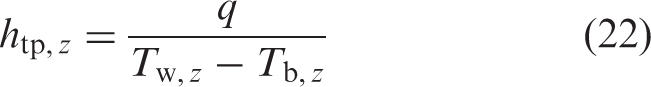
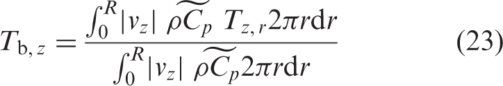
Figure 4 shows the axial distribution of the local heat transfer coefficient calculated using equation (22)
Validation of the CFD heat transfer model of steady, laminar, fully developed annular flow using the analytical model of Gupta.
50
The CFD heat transfer coefficient profile is obtained at t = 100 ms.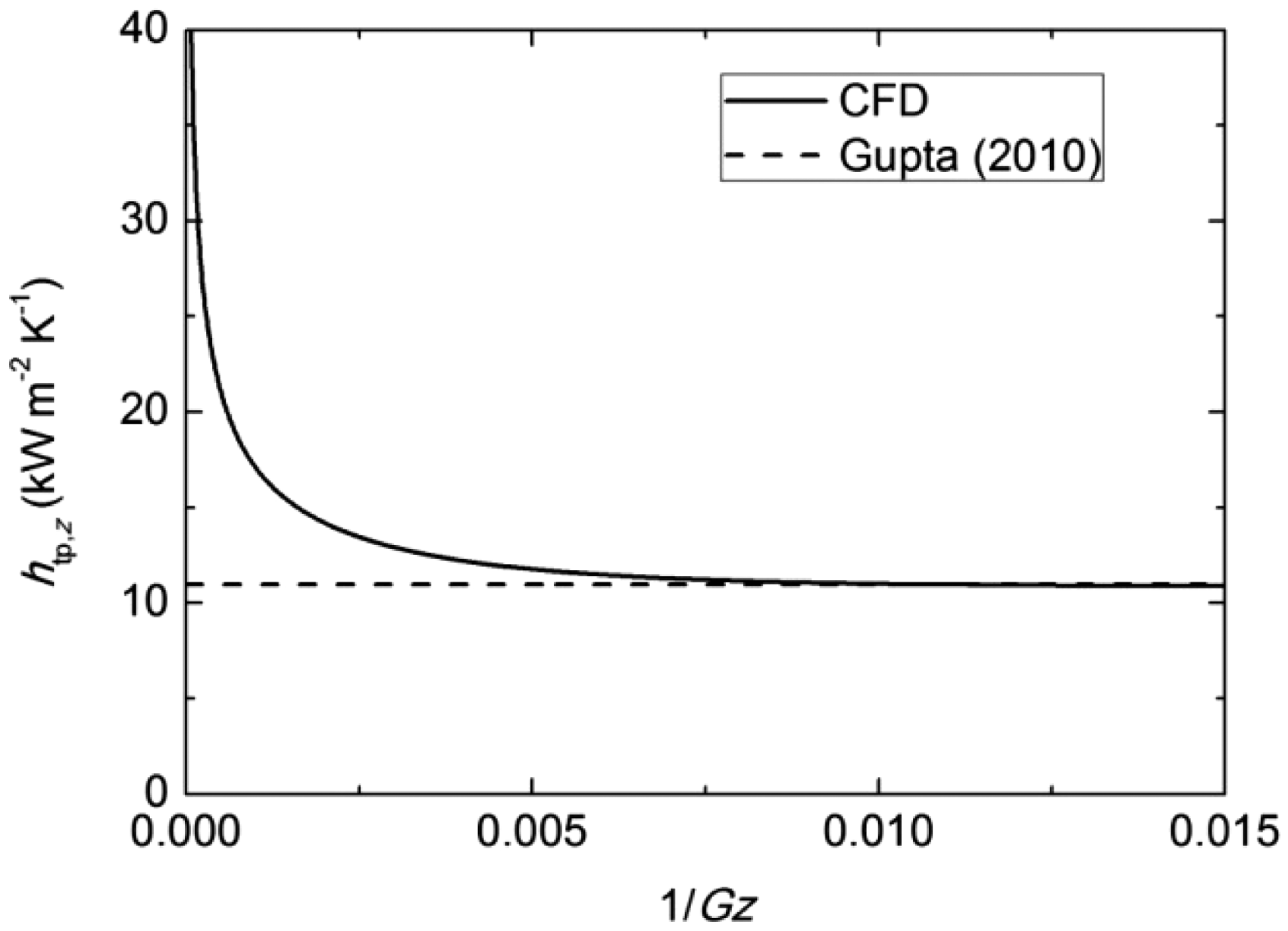
Assessment of the impact of interface perturbations
Boiling simulations are performed using the dimensions and inlet conditions for the case described in the ‘Steady, laminar, fully developed annular flow heat transfer without phase change' section with the phase change model enabled. In addition, inlet perturbations (amplitude
Figure 5(a) shows the evolution of the total vapour mass source with time for the steady and perturbed inlets. After t = 40 ms, the vapour source for the constant inlet case reaches a plateau with only small fluctuations. With the imposition of inlet fluctuations, the overall vapour mass sources become periodic after t = ∼50 ms, indicating that the flows are quasi-steady. The oscillation frequencies of the source for both perturbation cases are similar, but the magnitudes of the source of the fixed liquid flow rate case are slightly higher than those of the fixed pressure gradient case. Fast Fourier Transform (FFT) analysis shows that the source frequencies for both perturbation cases are ∼10 ms which is equivalent to the perturbation frequency. The average magnitudes of the sources in the quasi-steady phase of the three cases are not exactly the same because the mean mass flow in the three cases is not identical.
Exploration of the annular flow boiling model for water at 101.3 kPa with Ul = 0.11 ms−1 and Ug = 6 ms−1; D = 1 mm and wall heat flux of 25 kW m−2. (a) The evolution of vapour mass sources with time for different inlet perturbation conditions. The axial wall temperature at t = 100 ms profiles for all four cases is shown in (b).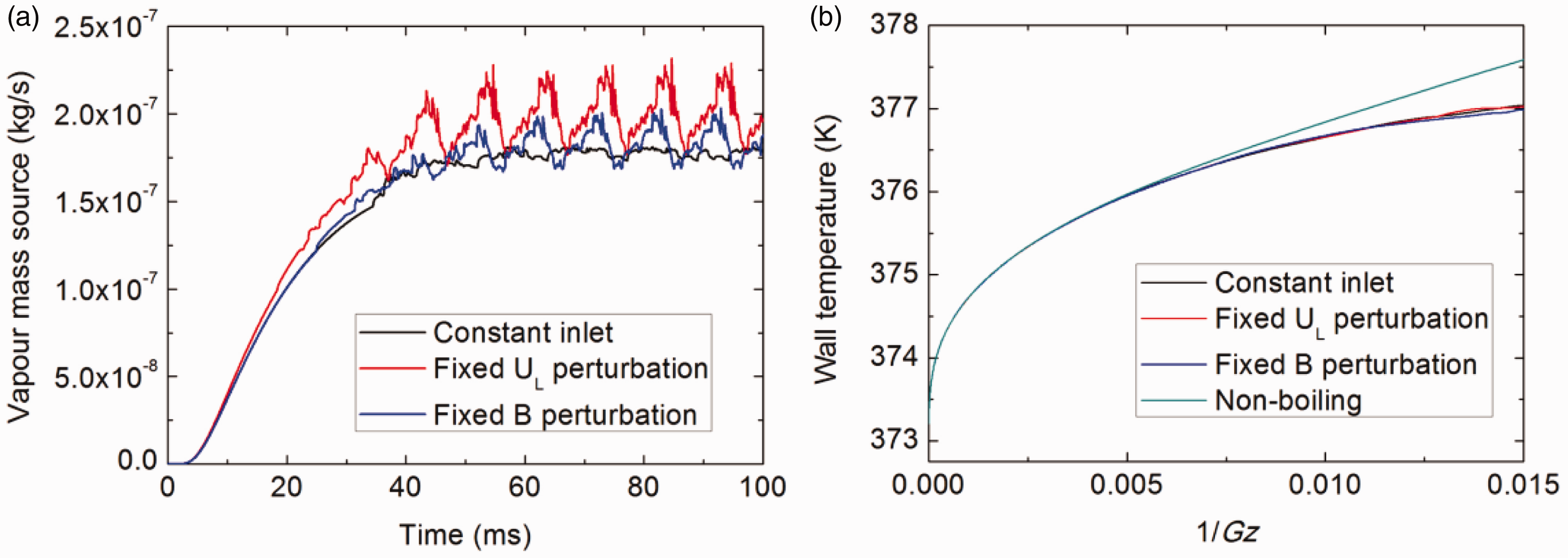
Figure 5(b) shows the axial wall temperature distribution for all three boiling cases at t = 100 ms, with the non-boiling results also shown for comparison. At low values of
Boiling heat transfer
In annular flow boiling, the vapour quality increases along the flow direction due to the continuous heat input. For a channel with diameter D and length LA, assuming all heat input is used to vaporise the liquid, the boiling mass transfer rate (
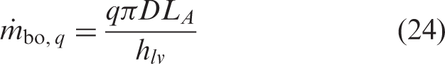
The change in vapour quality (
In the following sections, we consider boiling of water at 160 kPa (
Transient behaviour of annular flow boiling in microchannels
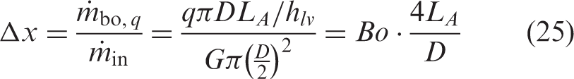
Figure 6 shows the evolution of the global mass source calculated using equation (21). Beyond the initial transient discussed previously, the global source reaches a peak value at t = ∼12 ms after which it reaches an approximate (±10%) plateau. The dashed line, denoting the theoretical boiling mass source
Evolution of the amount of vapour mass source in the computational domain (D = 0.5 mm, Ug = 6.55 ms−1, Ul = 0.057 ms−1, q = 20 kWm−2, x = 0.1). The dashed line denotes the calculated boiling source
Characterisation of local boiling heat transfer at t = 30 ms for a microchannel boiling annular flow (D = 0.5 mm, Ug = 6.55 ms−1, Ul = 0.057 ms−1, q = 20 kWm−2, x = 0.1). (a) The temperature field and the local boiling heat transfer coefficient distribution along the axial direction. (b) Local heat transfer coefficient distribution and the temperature and velocity fields near the wave crest in the dashed rectangle in (a). The black solid lines in the temperature contours denote the gas–liquid interface. The axial length of the channel was scaled by a factor of 0.25 and 0.5 for (a) and (b). The display density of the vector field in (b) was reduced for better presentation.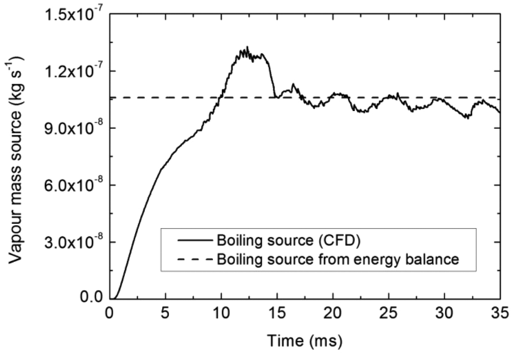
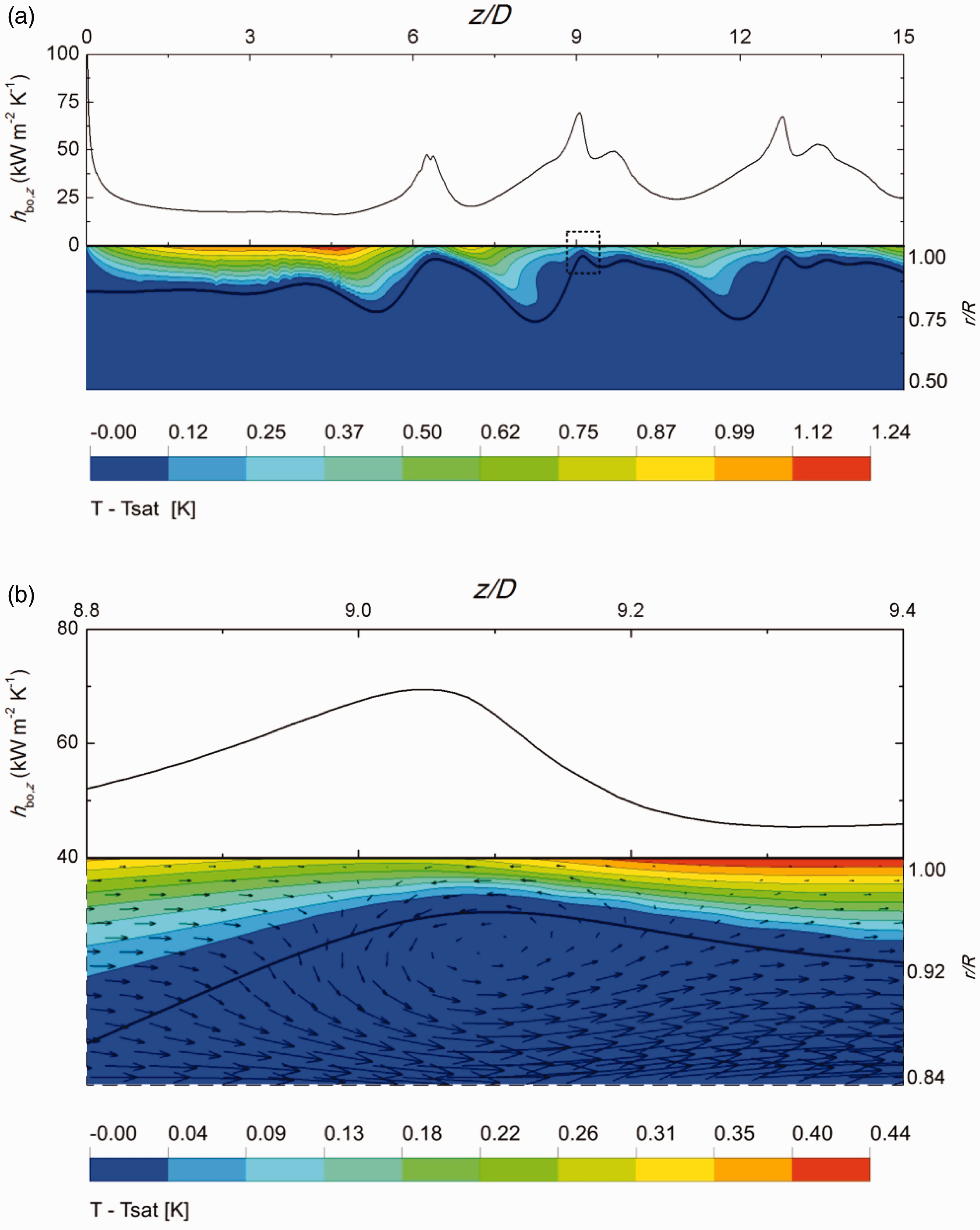
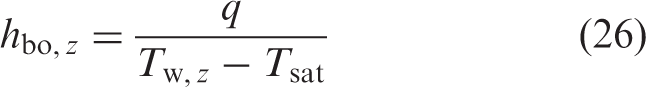
Figure 7(a) also shows the distribution of local boiling heat transfer coefficient calculated using equation (26)
Determination of developed flow and average boiling heat transfer coefficient
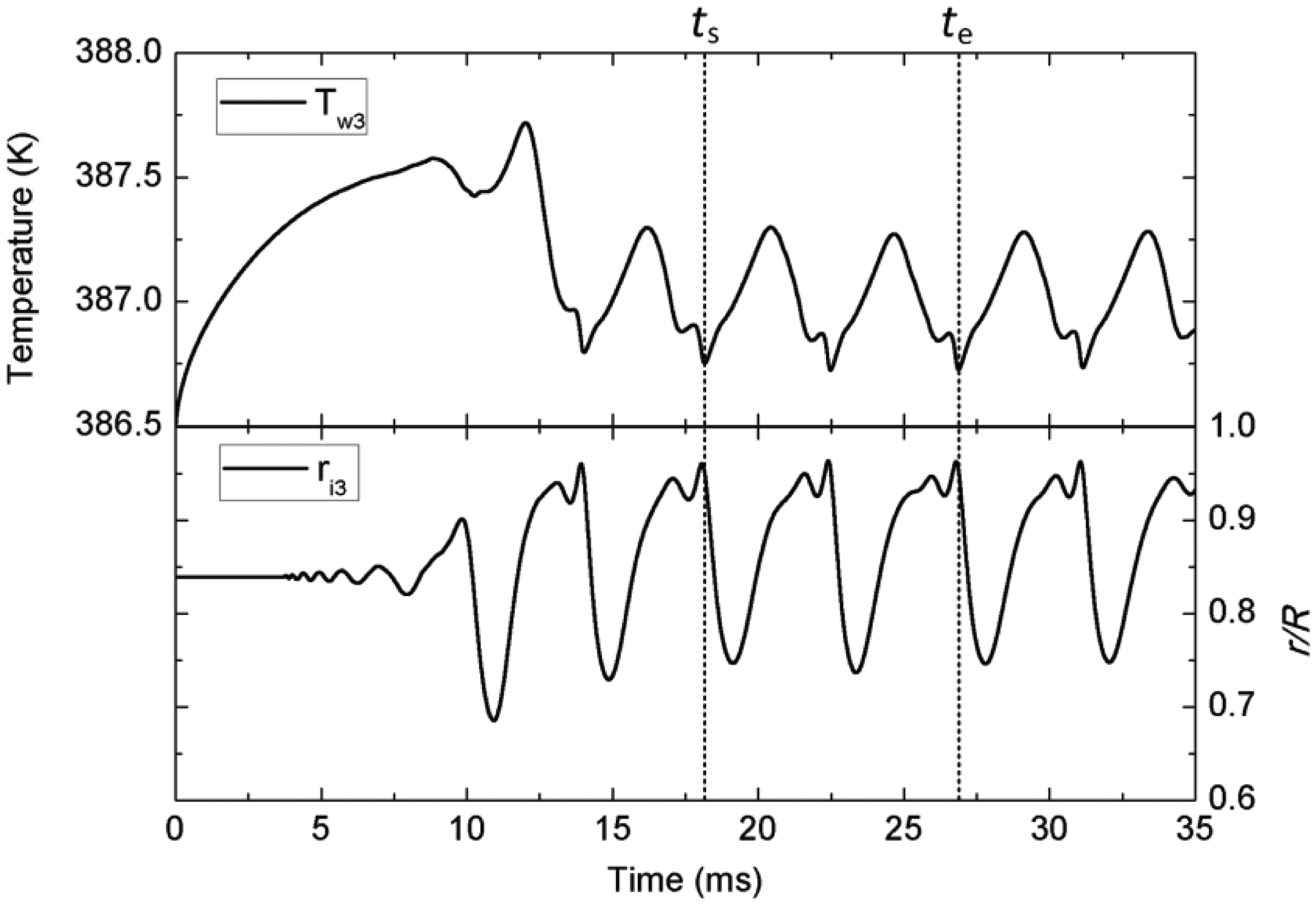
As the interfacial waves shown in Figure 7(a) are advected by the flow, the local heat transfer coefficient becomes time-dependent due to the oscillating interface radius at the same axial location. To characterise the time-dependent interfacial radius and the corresponding local heat transfer, monitor point pairs are placed at
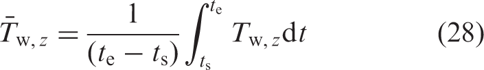
The monitored wall temperature and interface radius at the same axial location
Fast Fourier transform (FFT) analyses of the respective periodic behaviours are shown in Figures 9(a) and 9(b) for interface location and wall temperature, respectively. The same dominant frequency of ∼250 Hz is seen in every case, indicating the generation and advection of regular waves at the gas–liquid interface. The amplitudes of the component frequencies are shown in Figures 9(c) and 9(d). These are smallest at the first axial location (
FFT analysis for the interface radius and the wall temperature variations at four axial locations. The power spectral densities (PSD) for the interface radius and the wall temperature are shown in (a) and (b), respectively. The amplitudes of the component frequencies are shown in (c) and (d).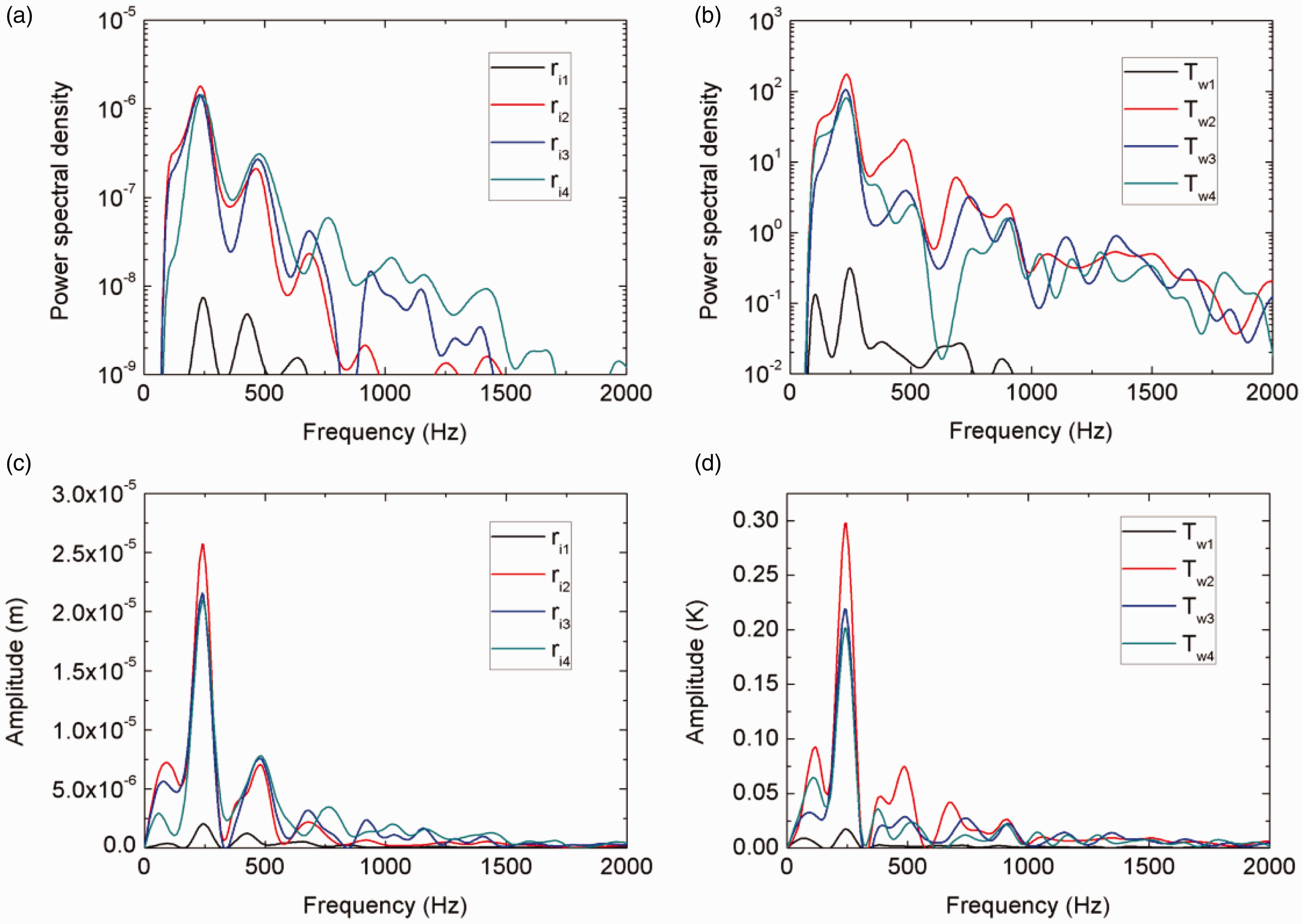
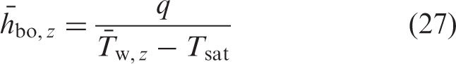
The average boiling local heat transfer coefficient for a monitored axial location can be calculated using equation (27)
Average heat transfer coefficients at different monitored axial locations.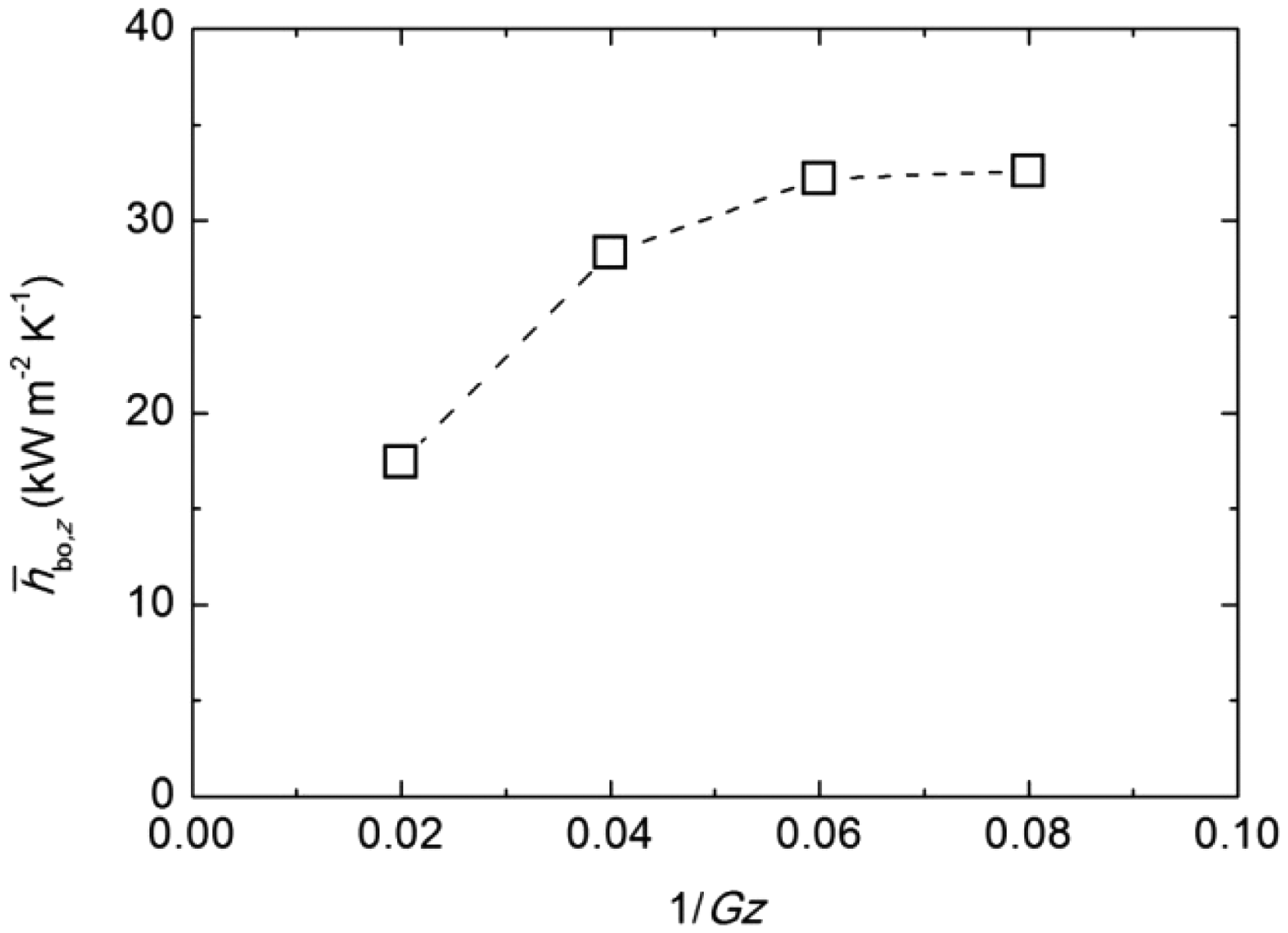
Heat transfer enhancement caused by the interfacial waves
For steady-state conduction across a thin laminar film of thickness
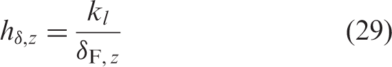
Figure 11 shows this comparison for the axial location of
Comparison of local heat transfer coefficient between annular flow boiling and film conduction model at the axial location of
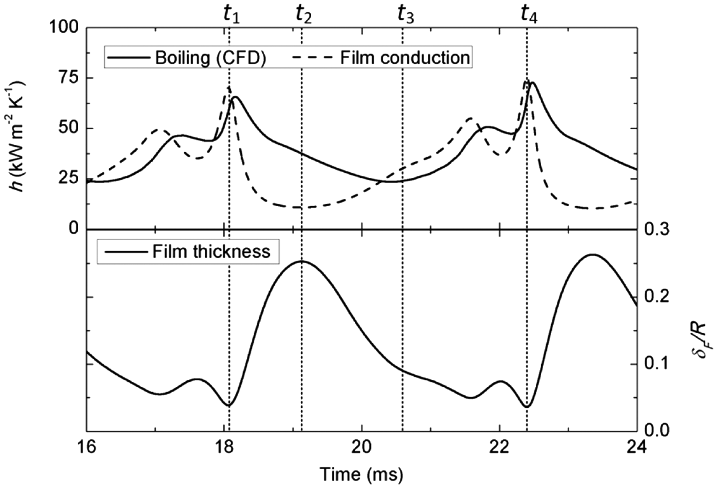
The average local film thickness calculated using an approach similar to the average wall temperature (equation (28)) yields
Origin of the waves
The mechanism by which waves form in the absence of any introduced perturbation requires investigation. The question is whether this is a numerical artefact or something that represents a physical phenomenon. In order to investigate this, a number of test cases were performed as follows:
A simulation was performed in which the boiling source was calculated based on the boiling number and applied at the cell in which the interfacial area was highest at each radial location. Source term smoothing and shifting were disabled. No waves were generated. The above case was modified to apply the source at all cells with a non-zero interfacial area and the source was weighted by the cell value of the interfacial area. This saw the source being spread over several cells but no waves were generated. Visualisation of the source terms in a standard boiling simulation showed that prior to shifting and smoothing locally, high evaporation sources could occur in cells where the interfacial area was non-zero in a cell closer to the wall than its neighbours. Examination of the components of the source showed that the evaporation flux jm increases rapidly towards the wall so that any small interfacial area term in a cell nearer to the wall can cause a large source term locally. Even though this effect is reduced in the smoothing step, there are still locally high sources. This potentially explains a mechanism in which locally high source terms can generate instability at the interface. Quantitative examination of the source components of five adjacent interfacial cells at the liquid side shows an average temperature jump of ∼0.015 K between these neighbouring cells, corresponding to a mass flux difference of ∼0.1 kgm−2s−1. Compared with the average evaporation mass flux of ∼0.012 kg m−2 s−1 over the interface, this difference shows the high sensitivity of the evaporation mass flux to the interface temperature variation and could cause local perturbations to the interface by changing the volume fraction values of the interfacial cells non-uniformly. A standard boiling simulation was run in which the momentum source terms were suppressed. These can potentially play a role in generating instabilities as explained in Granovskii et al.
51
However, even in this case, wave formation was still observed. The interfacial area is represented using the gradient of the volume fraction and it is known that this will diffuse the interface across several numerical cells. It is possible to use other functions that provide a much sharper interface. To test the impact of this, the interfacial area density was calculated using
A calculation of local mass flux using the evaporation model used by Hardt and Wondra
46
yields identical results to that obtained using the current phase change model, confirming that no additional instabilities are introduced by using the pressure difference form of the Tanasawa
39
model instead of using the temperature difference form. A boiling case performed with the phase change model disabled in the near-inlet region (0 <
The boiling simulation was run with the phase change kinetic coefficient (
In summary, these tests have shown that neither the phase change model nor the numerical smoothing procedure have introduced numerical artefacts that generate waves. However, the observed high sensitivity of evaporation mass flux to the interface temperature has shown large potential for the generation of local perturbation when the interfacial area moves into a cell near the wall. If this happens, the rapid local increase of the evaporation mass flux causes a very high local evaporation flux and thus acts as a perturbation to the interface. In any real system, there are a variety of sources of possible perturbations, such as non-uniformity of the wall heat flux, wall surface finish variations, 3D perturbations to the flow, etc. that could provide the slight asymmetries needed to induce wave formation. We therefore proceed on the basis that the waves generated are a consequence of the physical modelling assumption.
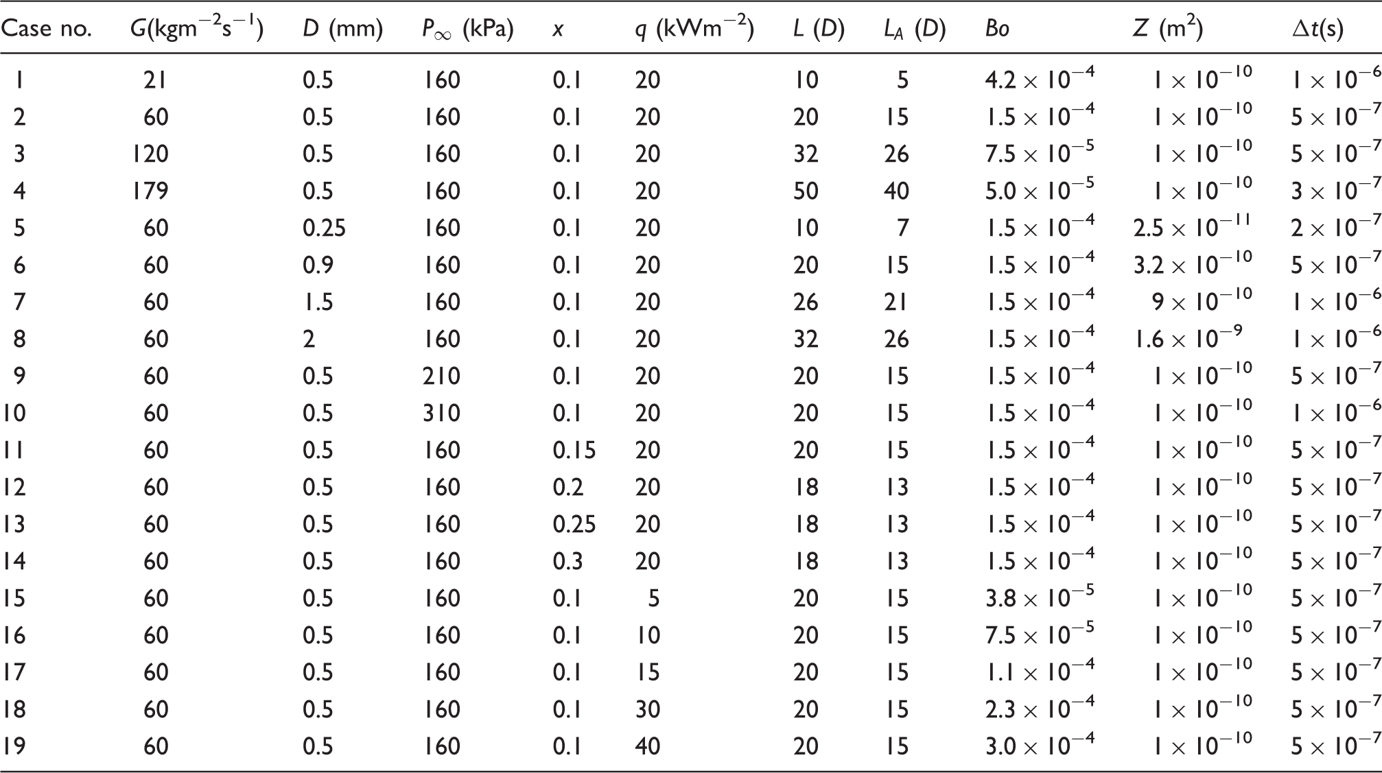
Parametric analysis of annular flow boiling heat transfer
List of cases used for the parametric analysis.
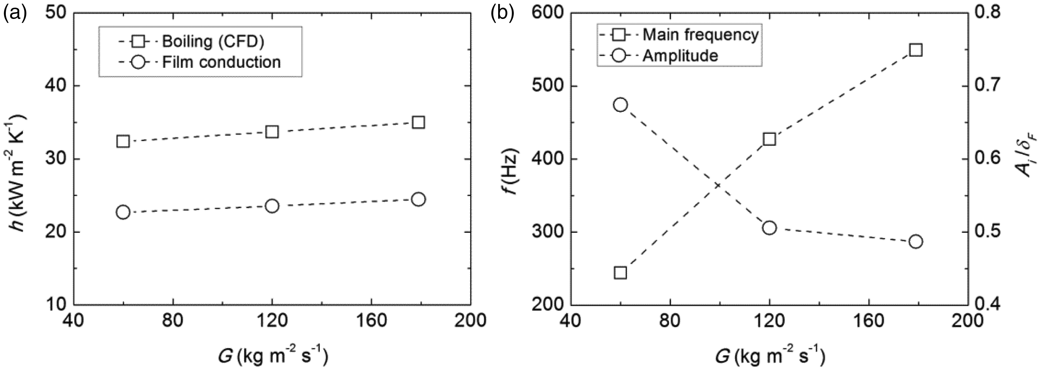
Effect of mass flux
Figure 12 shows the effects of varying the mass flux from 60 to 179 kgm−2s−1. The data from Case 1 are not plotted because the low superficial velocity led to a slug-annular flow in the simulation. Overall, it is found that both boiling and film conduction heat transfer coefficients increase slightly with increasing mass flux. This effect is correlated with higher interfacial wave amplitudes relative to the average film thickness, In addition, the frequency of the waves increases with increasing mass flux, as shown in Figure 12(b). The enhancement factor (
Effect of fluid mass flux (cases 2–4) on annular flow boiling (D = 0.5 mm,
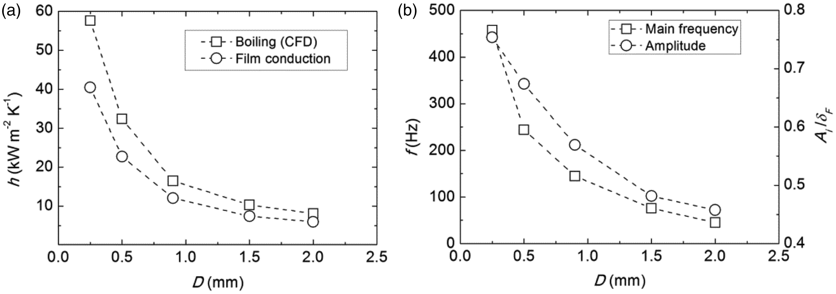
Effect of tube diameter
Figure 13(a) shows that the boiling heat transfer coefficient decreases significantly as the channel diameter is increased from 0.25 mm to 2 mm. The increase in film thickness with increasing tube diameter is the main reason for this effect but the smaller relative amplitude of the waves, Figure 13(b), also contributes. Figure 13(b) shows that the frequency of the interfacial waves varies inversely with channel diameter, suggesting an approximately constant value of Strouhal number,
Effect of channel diameter (cases 2 and 5–8) on annular flow boiling (G = 60 kgm−2s−1,
Effect of system pressure
Figure 14(a) shows that the simulated boiling heat transfer coefficient increases with pressure in the range 160–310 kPa, even as the film thickens and the film conduction heat transfer coefficient decreases slightly. These opposing trends arise because the interfacial wave amplitude increases as the pressure increases, as shown in Figure 14(b). At the same time, the inlet superficial gas velocity decreases from 6.55 ms−1 to 3.52 ms−1 and the wave frequency shown in Figure 14(b) also decreases. The enhancement factor between the boiling and film conduction heat transfer coefficients increases from 1.43 to 1.91 with increasing pressure.
Effect of system pressure (cases 2 and 9–10) on annular flow boiling (G = 60 kgm−2s−1, D = 0.5 mm, x = 0.1, q = 20 kWm−2): (a) boiling and film conduction heat transfer coefficients; and (b) main frequency and the corresponding amplitude of the interfacial waves.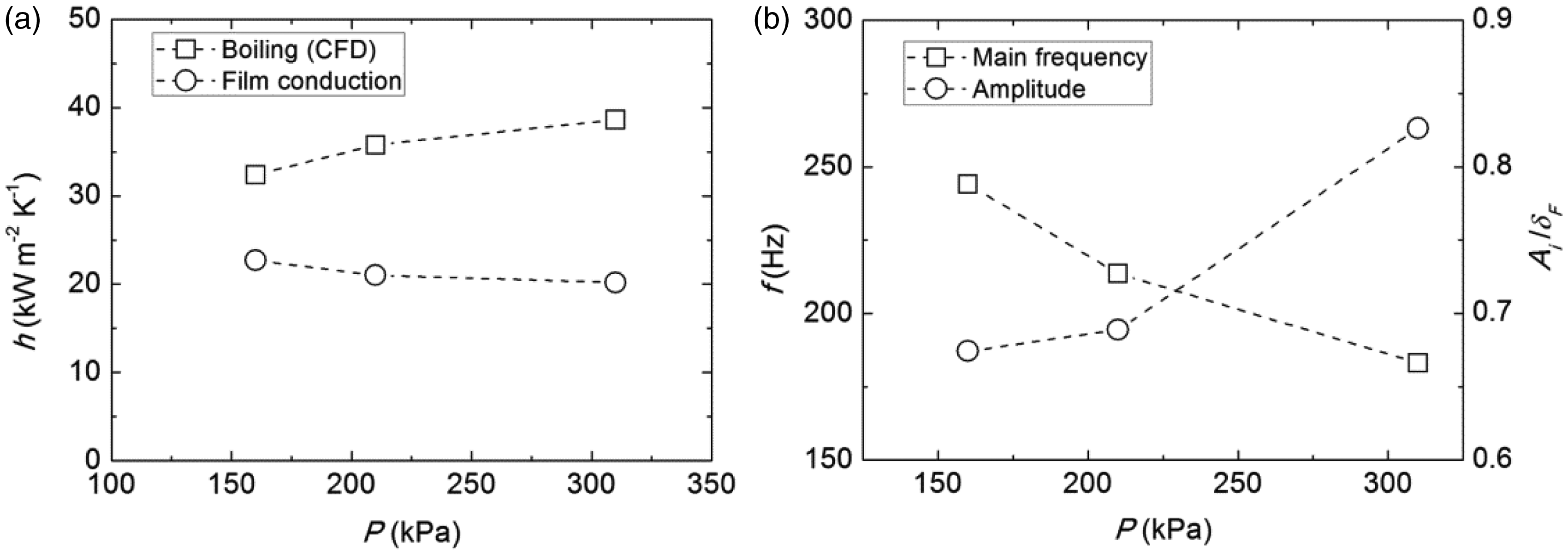
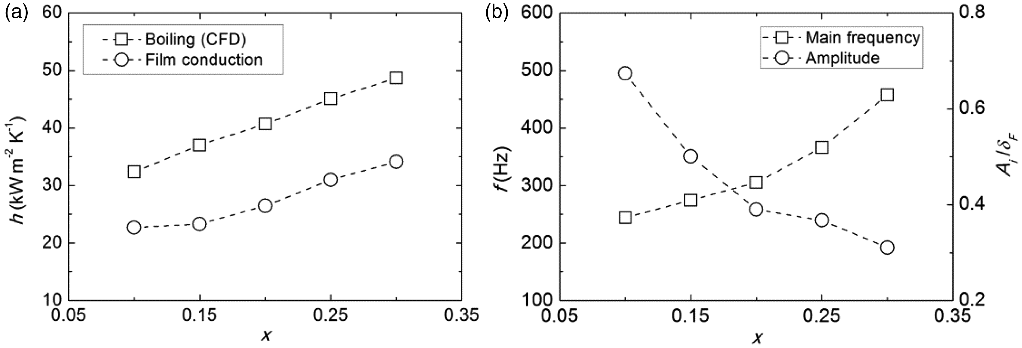
Effect of vapour quality
In the simulations, the mean liquid film thickness decreases significantly with increasing vapour quality due to higher gas superficial velocity and lower liquid superficial velocity. Therefore, as shown in Figure 15(a), the film conduction heat transfer coefficient increases with increasing vapour quality, as does the simulated boiling heat transfer coefficient. The non-dimensional wave amplitude is shown to decrease with increasing vapour quality in Figure 15(b), indicating that the film is relatively smoother at higher quality. Figure 15(b) also shows that higher wave frequencies are predicted with higher vapour quality. The enhancement factor ranges from 1.43 to 1.59.
Effect of vapour quality (cases 2 and 11–14) on annular flow boiling (G = 60 kgm−2s−1, D = 0.5 mm,
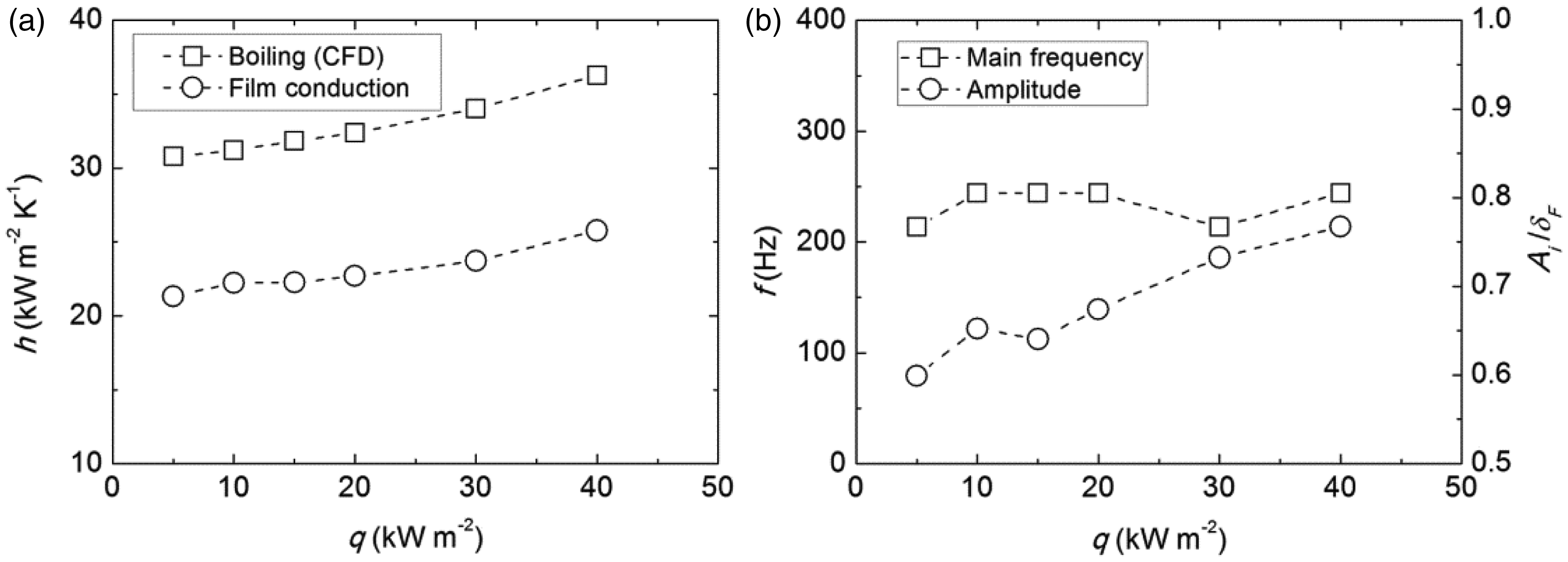
Effect of wall heat flux
The results from the variation of the wall heat flux are shown in Figure 16. Both boiling and film conduction heat transfer coefficients increase with increasing heat flux as the non-dimensional interfacial wave amplitude increases slightly with increasing heat flux (Figure 16(b)). The frequencies shown in Figure 16(b) have little dependence on the heat flux – since the gas velocity is also only slightly affected by the magnitude of the heat flux in these simulations. The enhancement factor stays in a narrow region between 1.40 and 1.44.
Effect of wall heat flux (cases 2 and 15–19) on annular flow boiling (G = 60 kgm−2s−1, D = 0.5 mm,
Comparison with correlations
In this section, the CFD results are compared with some of the existing correlations for the prediction of film thickness and the boiling heat transfer coefficient.
Liquid film thickness
Bang et al. 52 calculated the film thickness using the gas void fraction determined by the Lockhart–Martinelli approach. In their model, instead of using the conventional turbulent–turbulent form for the Martinelli parameter, an empirical expression proposed by Yu et al. 53 was used. In addition, Bao et al. 54 showed the CISE approach, recommended by Hewitt, 55 provided good estimates of void fractions in two-phase microchannel flows. In this section, the film thickness is calculated following the procedure of Bang et al., 52 with the gas void fraction determined by the Lockhart–Martinelli and CISE approaches above.
Figure 17 shows that the Lockhart–Martinelli approach predicts the CFD film thickness within ±20% error, whereas the CISE approach underestimates some data points by more than 20%. The increasing/decreasing trends in the parametric groups are captured correctly except for the wall heat flux cases where both methods predict a constant film thickness value because the heat flux effect is not included in either of them. The ratio of film thickness calculated in the CFD simulations to the predicted value (
Comparison of the CFD film thickness with those predicted by: (a) Lockhart–Martinelli, and (b) CISE approaches. Various symbol types are used to denote the values from different parameter groups: base case (▪), mass flux (□), tube diameter (^), system pressure (Δ), vapour quality (▽) and wall heat flux (⋄).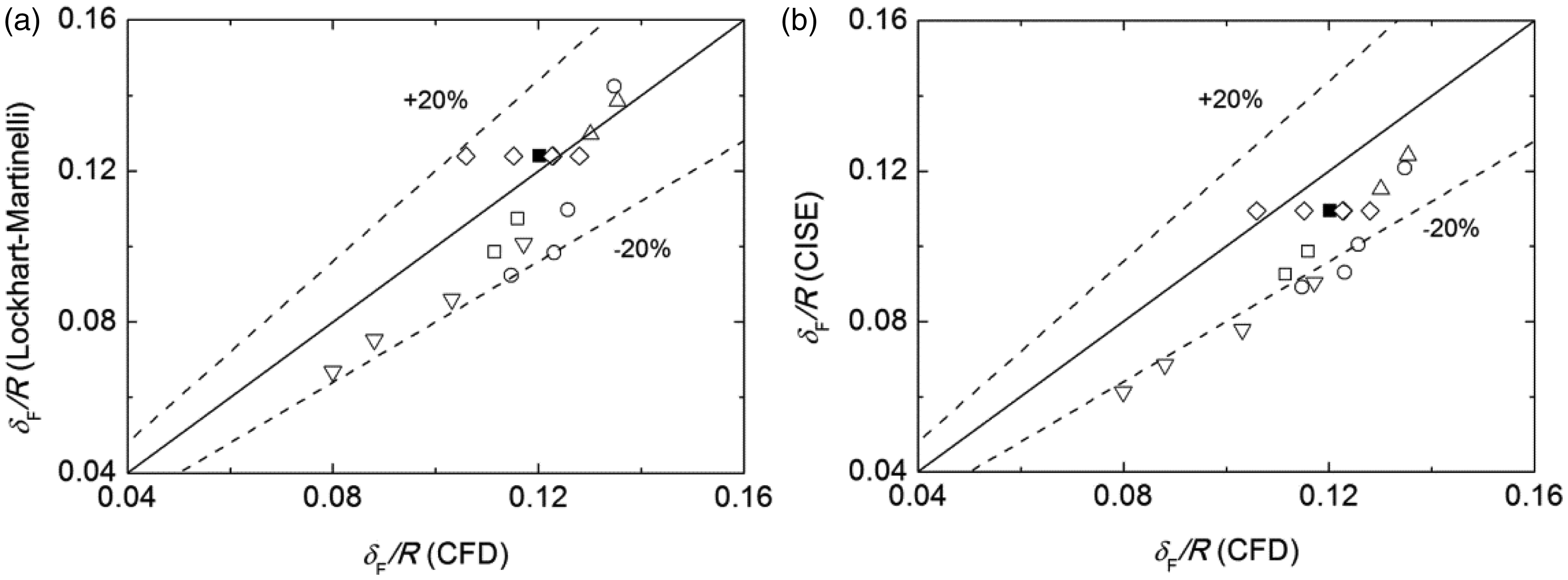
Heat transfer coefficient
A large number of correlations have been developed for the prediction of heat transfer coefficient in boiling flows. Reviews and discussion of the correlations are available in many works, such as Bertsch et al. 5 and Kim and Mudawar. 56 In the current work, the Kim and Mudawar, 56 Kandlikar and Balasubramanian, 57 and the Bang et al. 52 models are chosen for comparison with the current CFD results, because of their wide usage and validity ranges consistent with the current geometric and flow parameters. The Kim and Mudawar 56 model was constructed through reviewing a large number of existing correlations and covers various fluids and parameter ranges. The Kandlikar and Balasubramanian 57 model calculates the boiling heat transfer coefficient as an enhanced single-phase laminar heat transfer coefficient. The Bang et al. 52 model is a film conduction model with the film thickness being estimated using a modified Lockhart–Martinelli approach. Despite the consideration of both nucleate and convective boiling contributions in the first two correlations, only the convective parts are used here because the current CFD work assumes a completely convective boiling process. The film conduction heat transfer coefficient calculated using the average CFD film thickness is also used in the comparison.
Figure 18 shows the comparison between the CFD boiling heat transfer coefficients with the predicted values from the correlations. The Kim and Mudawar
56
correlation (Figure 18(a)) underestimates the CFD boiling heat transfer coefficient for most data points except the low values (<20 kW m−2K−1), whereas the Kandlikar and Balasubramanian
57
correlation (Figure 18(b)) overestimates the CFD data except for those from two pressure cases. The Bang et al.
52
film model (Figure 18(c)) underestimates all the CFD data by around 30%. It is noted that the vapour quality effect is weakly predicted by the Kim and Mudawar
56
correlation. More strikingly, the pressure effect predicted by the Kandlikar and Balasubramanian
57
correlation and the Bang et al.
52
film model is contrary to that for the CFD boiling heat transfer coefficients. As pointed out by Liu et al.
58
the correlations are developed based on a large number of experimental datasets obtained with various levels of upstream compressibility (“soft inlet” vs “hard inlet”) and have often been shown to provide poor predictions of any particular dataset. It is therefore not surprising that there are significant discrepancies between the predicted values and the current CFD results (which are obtained with a “hard inlet”).
Comparison of the CFD boiling heat transfer coefficients with those predicted from correlations: (a) Kim and Mudawar correlation
56
; (b) Kandlikar and Balasubramanian
57
correlation; (c) Bang et al.
52
film model; and (d) CFD film thickness model. Various symbol types are used to denote the values from different parameter groups: base case (▪), mass flux (□), tube diameter (^), system pressure (Δ), vapour quality (▽), and wall heat flux (⋄).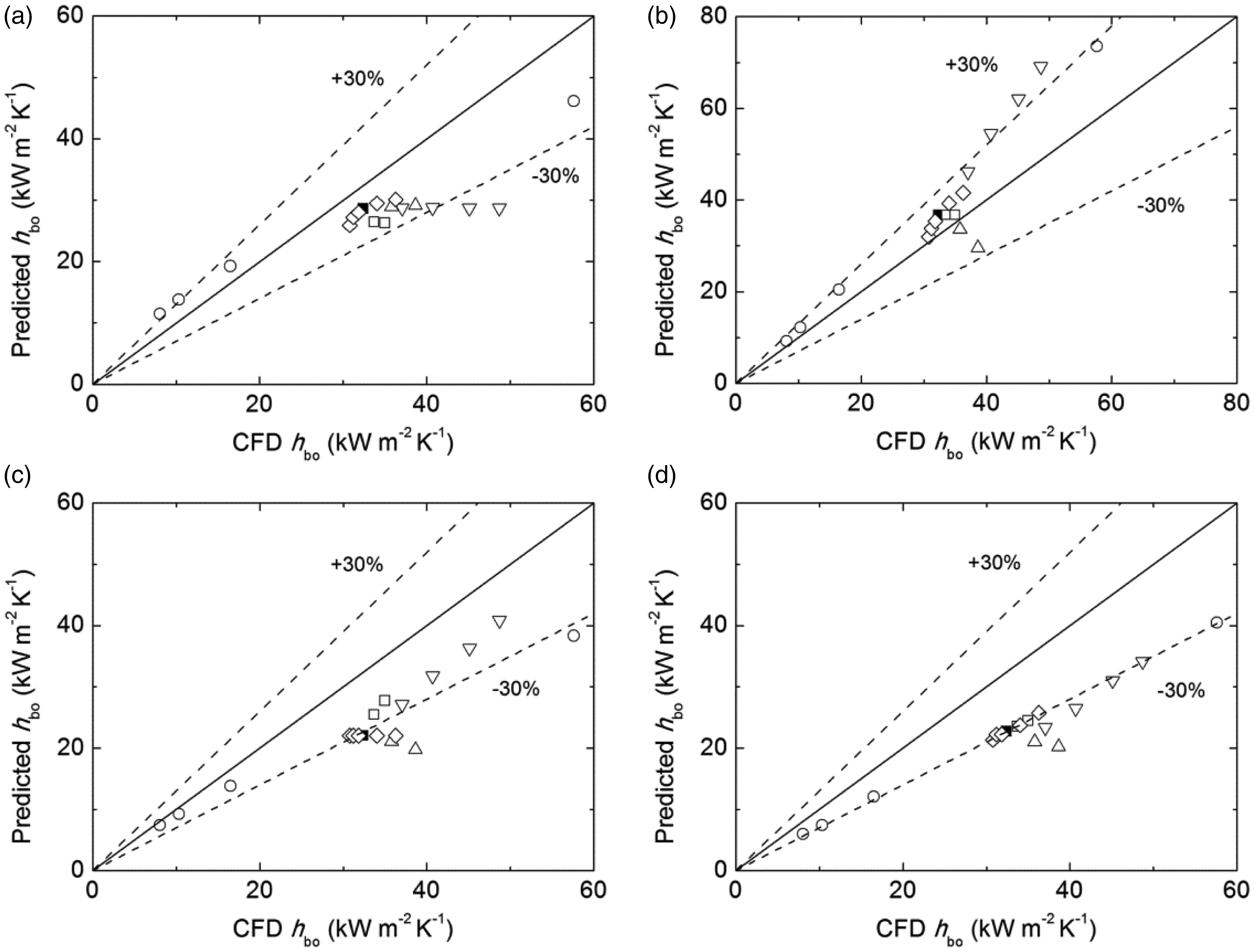
Notably, the predictions made by the CFD film thickness model (Figure 18(d)) are worse than those made by the Bang et al. 52 film model. In fact, it is shown in the ‘Heat transfer enhancement caused by the interfacial waves' section that the boiling heat transfer coefficient is higher than the film conduction value due to the heat transfer enhancement made by the interfacial waves. The average enhancement factor for the film conduction coefficient found in the simulations is 1.48 (standard deviation 0.14, 18 points).
It is evident that none of the correlations or the simple film thickness model can capture the behaviour observed in the CFD simulations. This is hardly surprising given the massive scatter seen when the correlations are compared with experimental data and the simple film model ignores the enhancement arising from the interfacial waves. Work is underway using the apparatus described in Liu et al. 58 to obtain experimental data for comparison using a hard inlet.
Conclusions
The CFD model developed in the current work has been applied to the analysis of convective flow boiling heat transfer in laminar, quasi-steady annular flow with interfacial instabilities caused naturally by either phase change or imposed numerical perturbation. Small inlet perturbations have a negligible effect on boiling heat transfer using the current model. Natural instabilities, which are caused by variations in the phase change mass flux at the interface, have shown significant enhancements to the overall heat transfer coefficient through the advection of interfacial waves that continuously reduce the film thickness and generate flow recirculation around them. The time-averaged boiling heat transfer coefficients obtained in the quasi-steady region have shown significant enhancement compared with the values obtained from a steady film conduction model.
Parametric analysis using the numerical model have shown positive effects of increasing mass flux, system pressure, vapour quality and wall heat flux, but negative effects of increasing channel diameter on the heat transfer coefficient. Comparisons have shown reasonable agreements between the CFD results and some existing correlations for the film thickness and the boiling heat transfer coefficient, even though some of the correlations were developed based on large number of experimental data obtained with unknown upstream compressibility. However, it failed in capturing effects of some parameters, such as vapour quality and pressure. A relatively constant enhancement factor (∼1.5) is obtained between the boiling model and the film conduction heat transfer coefficient.
Although the current model is only 2D and applies only to laminar flow, it has significant potential for the analysis of detailed mechanisms of microchannel flow boiling and the effects of various flow parameters. This model is also an excellent basis which could be extended to 3D to study asymmetric behaviour of boiling annular flows, such as wave crest stripping of droplets, and their effects on microchannel heat transfer.
Footnotes
Acknowledgements
Computational resources used in this work were provided by Intersect Australia Ltd. Z. Guo also acknowledges the China Scholarship Council and the University of Sydney.
Declaration of Conflicting Interests
The author(s) declared no potential conflicts of interest with respect to the research, authorship, and/or publication of this article.
Funding
The author(s) disclosed receipt of the following financial support for the research, authorship, and/or publication of this article: The work was supported under the Australian Research Council Discovery Grant DP120103235.