
Abstract
As for the gantry-type machine tools, the forces of the slide blocks supporting the beam are different for different saddle locations, which would further affect the stiffness of the slider–guide joints and the dynamic characteristics of the whole machine tools. Therefore, the beam kinematic joints (the slider–guide joints) on the gantry-type machine tools are crucial for the dynamics prediction of traveling bridge systems. In this article, considering the effect of axis coupling force on the slider–guide joints’ stiffness, an equivalent dynamic model of traveling bridge systems for the gantry-type machine tools is established using hybrid element method. The additional load variation in the four slider blocks is analyzed for different locations of the saddle, and the variation in the slider–guide joints’ stiffness and traveling bridge system natural frequency are also studied. Finally, validation experiments are conducted on the traveling bridge systems of the gantry-type milling machine tools, and the results show that the dynamic modeling proposed in this article can reach a higher accuracy.
Introduction
The computer numerical control (CNC) machine tool is composed of many components by fixed joints and kinematic joints. Therefore, the parameters of the joints, especially for kinematic joints, are very crucial for the machine tool dynamics which is complicated 1 and play an important role in the surface quality and machining accuracy of the parts2–4 and the stability of machining process. 5 Resonance and chatter must be avoided during the machining process; hence, the natural frequencies of the machine tools should be acquired. In order to predict and avoid the resonance and chatter, the dynamics of the machine tools in the design stage must be obtained by simulations or prototype testing. So, a volume of research has been conducted on the machine tool dynamics.
Using finite method, Mi et al. 6 analyzed the influence of preload of screw–nut joints and slider–guide joints on dynamic characteristics of a horizontal machining center, and the results show that the preloads have significant effects on the horizontal machining center dynamic stiffness. The effect of slider–guide joints’ preload on the dynamic of the machine tools or subsystem was analyzed by Lin et al. 7 and Hung and colleagues8,9 using finite method. Zhang et al. 10 presented a systematic procedure to predict the dynamic behaviors of a whole machine tool structure using receptance synthesis method, in which the dynamic model is composed of the distributed mass beams, lumped masses and joints. Considering the tool–holder joint interface, a dynamic model using distributed parameters was built by Ahmadi and Ahmadian 11 to predict the machine tool dynamic properties in various tool configurations. In order to predict the dynamics of a high-speed machine tool, Zaghbani and Songmene 12 presented a methodology for estimating the machine tool modal parameters during machining operation using operational modal analysis.
Obviously, the states of the machine tool are different during the machining process. The different states will lead to the different static and dynamic characteristics for the machine tools; therefore, the finite element dynamic model based on single state cannot predict these variations. Tlusty et al. 13 studied the serial and parallel kinematics for the machine tools and concluded that the stiffness behaves differently owing to the position variation in 1999. In 2006, Chanal et al. 5 studied the static stiffness variation in a machine tool for high-speed machining and provided the static stiffness maps for a given altitude z. In 2008, considering the deformation of the linear slider–guide joints and the bearing joints, Lu et al. 14 built the model of a hybrid machine tool with 3 degrees of freedom and analyzed the static stiffness during the machining workspace based on the stiffness matrix. Sanger et al. 15 analyzed the distribution of the stiffness for different types of parallel machine tools in order to find its weakness. Yigit and Ulsoy 16 employed a systematic procedure to evaluate the dynamic characteristics variation in a reconfigurable machine tool using a nonlinear receptance coupling, which includes the effects of weakly nonlinear compliant joints through the use of describing functions for the nonlinearities involved. Van Brussel et al. 17 studied the dynamics of a three-axis machine tool by using finite element method (FEM) and found that it possessed position-dependent dynamics. Using theoretical models, such as a simple mathematical model, a three-dimensional (3D) model and finite element models, Sriyotha 18 studied the dynamics of a coordinate measuring machines and concluded that its dynamics were highly dependent on its configuration in his doctoral dissertation. Symens and colleagues19,20 and Paijmans et al. 21 studied the dynamics variation in a machine with the position of the tool in its workspace for designing the high-performance motion controllers. Considering the varying dynamics, Da Silva et al. 22 discussed the integrated design of mechatronic system and pointed out that the dynamics variation affects the machine’s stability and performance. Law et al.23–25 researched the position-dependent dynamics and stability of serial–parallel kinematic machine and three-axis vertical milling machine tool considering the stiffness of kinematic joints as a constant value or without modeling the kinematic joints’ stiffness and also studied the structural design modifications and topology optimization of the column. 23 All these researches above made great contributions to the understanding of the static and dynamic characteristics of the machine tools.
These scholars analyzed the variation in dynamic characteristics for the machine tools from the angle of mass distribution, but not considering the effect of stiffness variation owing to the variation in mass distribution on the dynamics of the machine tools. On the other hand, Hung 9 and Dhupia et al. 26 found that the stiffness of the linear rolling guide joints exhibits a variation as a result of different preloads and external loads. Verl and Frey 27 found that the preloads of the screw–nut joints varied with the system feed rates through the experimental method in 2010. Zhang et al. 28 studied the dynamics of high-speed ball screw feed system and concluded that the system possesses velocity-dependent dynamics. In this article, therefore, a traveling bridge system of the gantry-type milling machine tools with three axes is taken as an example to study the effect of axis coupling force on the stiffness of the slider–guide joints and the dynamics (natural frequency) of the milling machine tools for different positions of the saddle. Finally, validation experiments are conducted for different saddle positions.
Dynamic modeling of traveling bridge systems considering the change in slider–guide joints’ stiffness
Equivalent dynamic model
In this article, a traveling bridge system of typical gantry-type milling machine tool is mainly composed of beam, saddle, headstock, spindle and ball screw feed system, as shown in Figure 1. The beam and the saddle can move along Y-axis and X-axis, respectively. The headstock can move along Z-axis on which the spindle is being carried. Because the force of the slide blocks supporting the beam changes when the saddle locates in different positions, the slide blocks’ stiffness also changes. So, the dynamics of the traveling bridge system should be discussed for different positions of the saddle in this article.
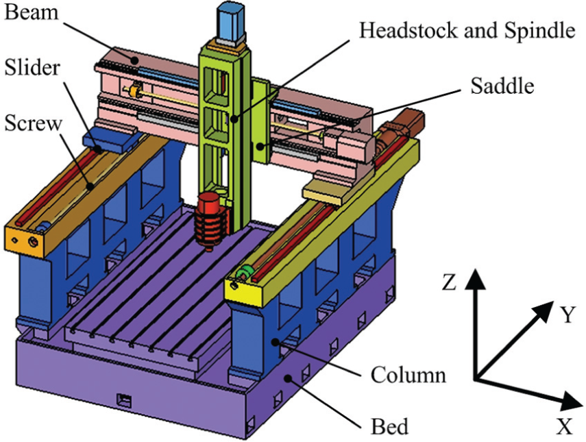
The gantry-type vertical milling machine tool.
The saddle is treated as a lumped mass element, and the headstock and spindle are also treated as a lumped mass element. The beam is equivalent to two spatial continuous beam elements with consistent mass distribution. The slider–guide joints are modeled by a set of spring–damper elements and the ball screw feed system is equivalent to a spring–damper element in transmission direction. Then, we can establish the equivalent dynamic model of the traveling bridge system for a typical gantry-type machine tool considering the effect of axis coupling force on slider–guide joints’ stiffness, as shown in Figure 2.
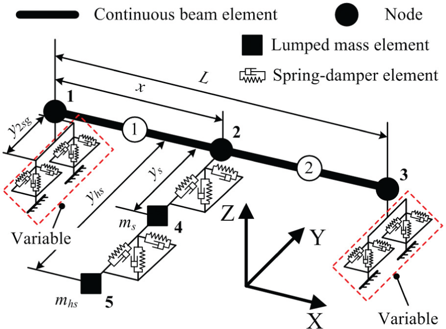
The dynamic model of the traveling bridge system.
In Figure 2, x is the distance between node 1 and node 2, L is the span between the two sliders of the Y-axis, y2sg is the distance between the two sliders, ys is the distance between the beam centroid and saddle centroid, yhs is the distance between the centroid of beam and the centroid of headstock and spindle, ms is the mass of the saddle, mhs is the mass of the headstock and spindle and ① and ② are the equivalent spatial continuous beam elements. 1–5 are the node numbers. Node 2 is a free node along the X-direction; in other words, the distance x between node 1 and node 2 is variable and it is decided by the position of the saddle. The stiffness of the spring–damping element in red dotted line in Figure 2 is variable with the saddle position.
Variable-coefficient dynamic equation
According to the equivalent dynamic model and D’Alembert principle, a variable-coefficient linear dynamic equation of the traveling bridge system can be established as equation (1) considering the change of slider–guide joints’ stiffness

where [M(x)], [C(x)] and [K(x)] are the system total mass, damping and stiffness matrix, respectively. They are a function of saddle position, and they are different when the saddle locates in different positions.
Calculation of the system mass and stiffness matrices
System mass matrix
Mass matrix of spatial continuous beam element
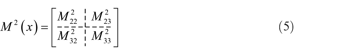
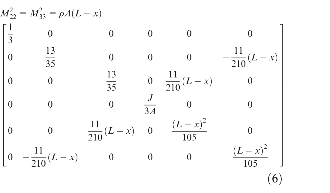
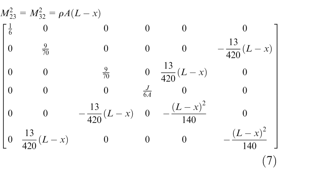
The mass matrices of element ① and ② are given by equations (2) and (5), 29 respectively
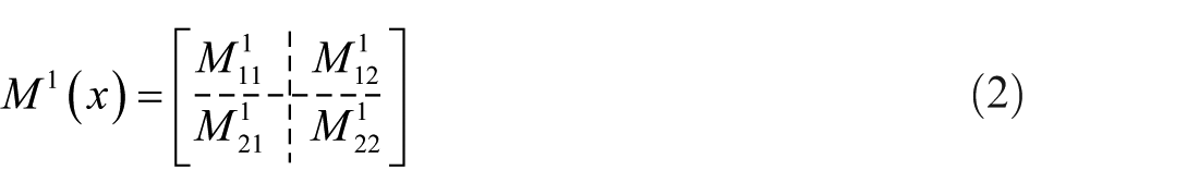
where
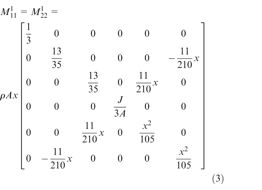
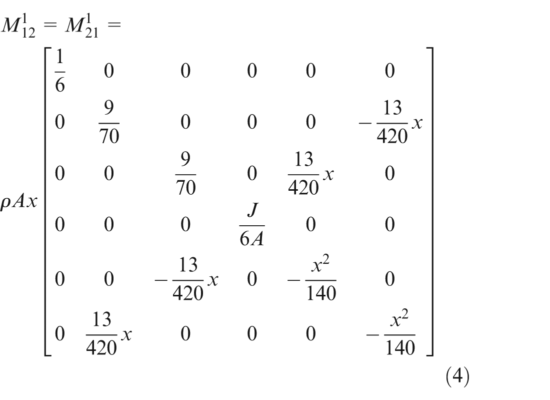
where ρ is the material density, A is the cross-sectional area of the beam element and J is the polar moment of inertia for beam element
where
System mass matrix
According to the mass matrix of each element, the expression of system mass matrix can be derived using the FEM 29
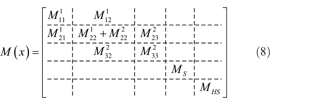
where MS and MHS are the matrix of the saddle and the matrix of the headstock, respectively. The moments of inertia for MS and MHS are ignored. Hence, the expressions of MS and MHS are given by equations (9) and (10), respectively
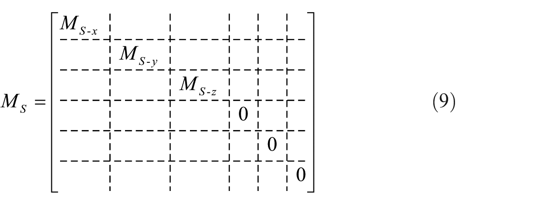
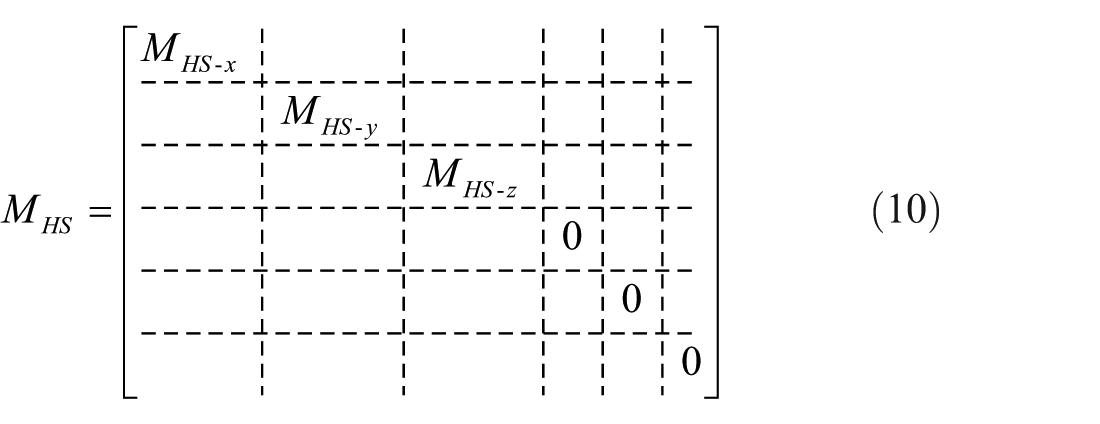
where MS-x, MS-y and MS-z are the mass of the saddle along X-, Y- and Z-directions, respectively. MHS-x, MHS-y and MHS-z are the mass of the headstock in X-, Y- and Z-directions, respectively.
System stiffness matrix
Stiffness matrix of spatial continuous beam element
The stiffness matrices of element ① and ② are given by equations (11) and (12), 29 respectively
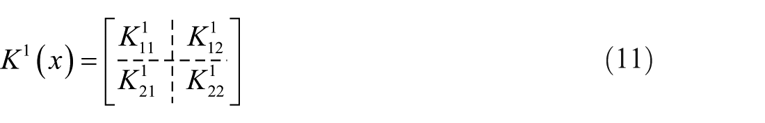
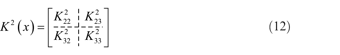
where
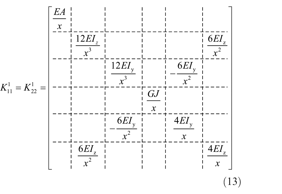
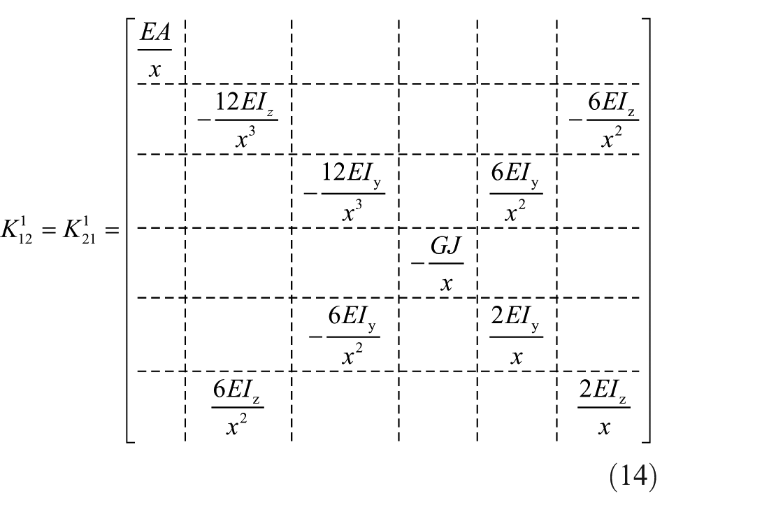
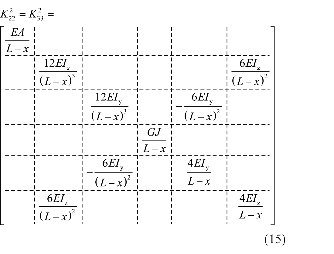
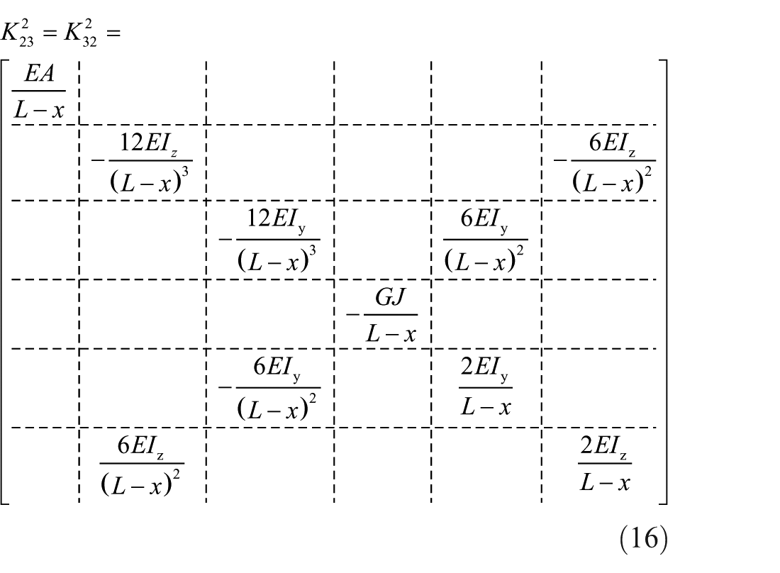
where E is Young’s elastic modulus and I is the moment of inertia for beam element.
Nonlinear stiffness of slider–guide joints for different saddle positions1The external loads of slider–guide joints
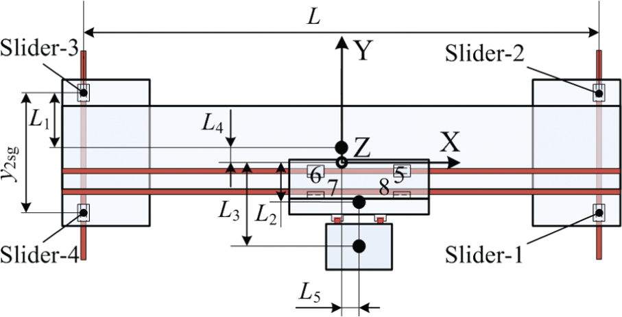
Figure 3 is the structure schematic diagram of the traveling bridge systems. The black dots in Figure 3 are the centroids of beam, saddle and headstock, respectively. The black circle in Figure 3 represents the center of the four sliders supporting the beam. L1 is the distance between the centroid of beam and slider 3 along the Y-direction. L2, L3 and L4 are the distance between the centroids of saddle, headstock and beam and the center of the four sliders along the Y-direction, respectively. L5 is the distance between the centroid of saddle/headstock and the center of the four sliders along the X-direction, and the distance changes with the machining process.
The forces act on every slider can be obtained by the following equations according to the size in Figure 3
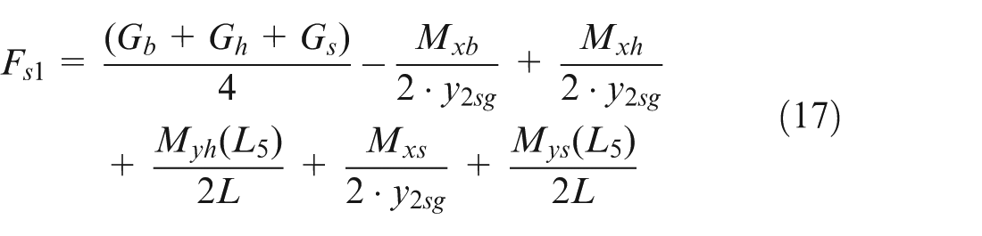
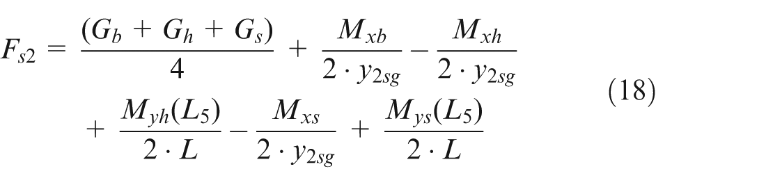
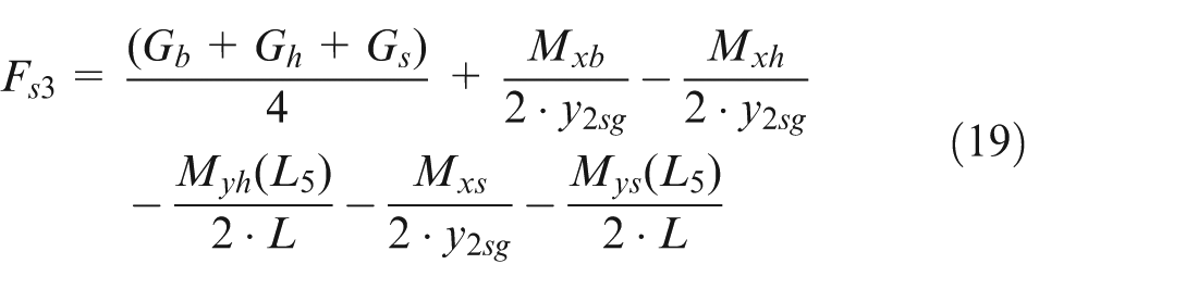
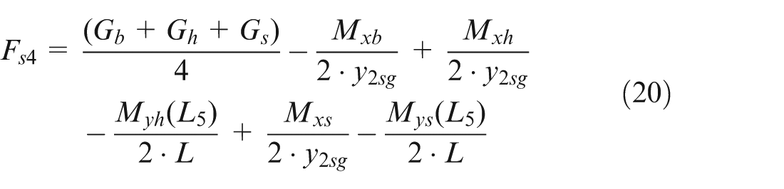
where Gb, Gh and Gs are the gravity of the beam, saddle and headstock, respectively. Mxb, Mxs and Mxh are the X-axial disturbance moment of the beam, saddle and headstock under the center of the four sliders, respectively. Mys(i) and Myh(i) are the Y-axial disturbance moment of the saddle and headstock under the center of the four sliders, respectively. The values of Mys(i) and Myh(i) vary with the machining process and they are a function of L5.
The nonlinear stiffness of slider–guide joints
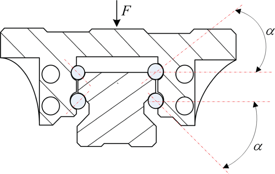
Figure 4 is the section schematic of circular arc-shaped linear guide with four rows.
The structure schematic diagram.
The section schematic of linear guide.
The contact force between a rolling ball and the raceway in the linear guide can be related to the local deformation at the contact point by the Hertz theory 30

where δ is the deformation, Q denotes the contact force and Kh represents the Hertz contact coefficient, which is determined by the contact shape and material properties of the linear guide components.31,32 So, the contact stiffness can be obtained by equation (22)
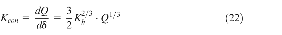
As shown in equation (22), the contact stiffness depends nonlinearly on the contact force. The contact force is composed of the initial preload and the additional load. The additional load varies with the position of saddle. Therefore, the additional contact stiffness also changes.
From Figure 4, we can derive the equivalent normal and tangential stiffnesses of a rolling ball in the linear guide as follows
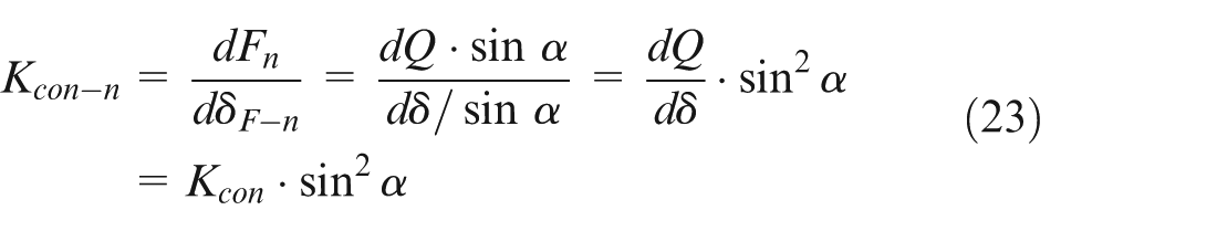
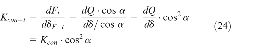
where α is the contact angle of linear guide. Fn and Ft are the equivalent normal and tangential forces of the contact force for a rolling ball, respectively. δF-n and δF-t are the equivalent normal and tangential deformations for a rolling ball, respectively.
System stiffness matrix
According to the stiffness of each element, the expression of system mass matrix can be derived 29 using the FEM
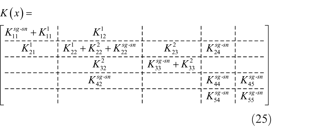
where
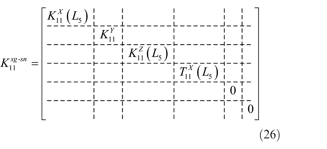
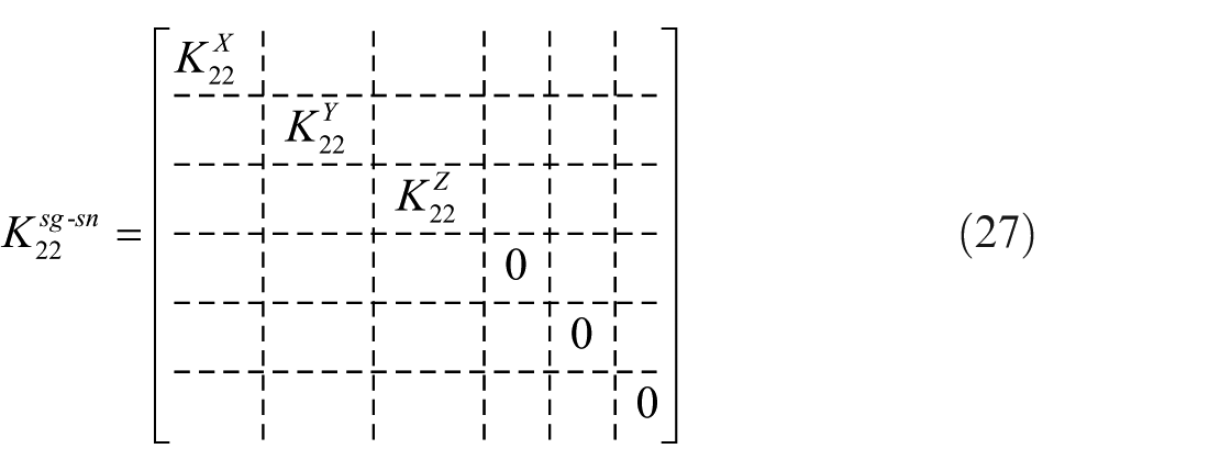
The
Experimental testing of traveling bridge systems for different locations of the saddle
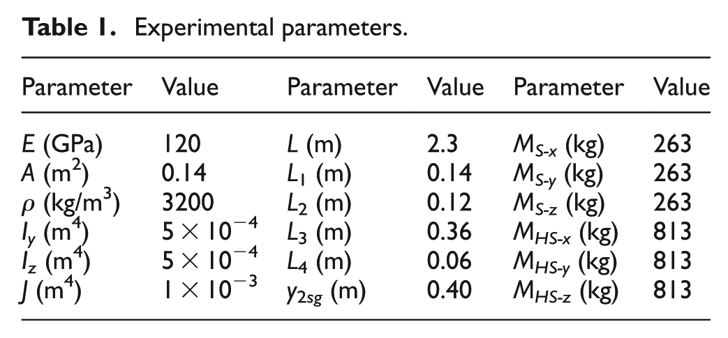
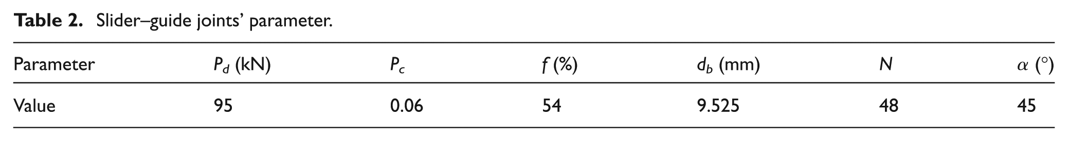
The traveling bridge system of the gantry-type machine tools was used to do the experimental testing, as shown in Figure 5. The parameters of the experimental setup are listed in Table 1. Table 2 represents the parameters of the slider–guide joints along Y/V-axis.
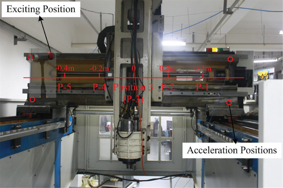
Hammer excitation test experiments.
Experimental parameters.
Slider–guide joints’ parameter.
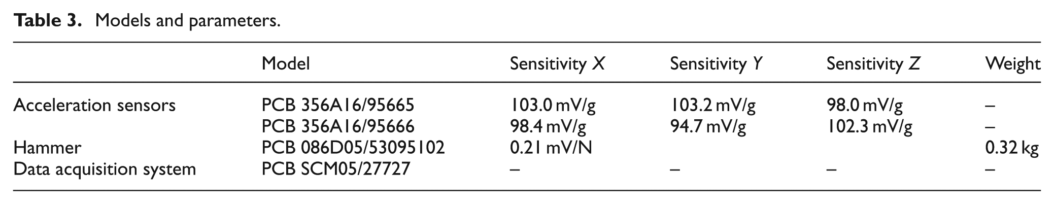
The dynamic characteristics of the traveling bridge system for different locations of the saddle were tested using LMS Test.Lab. The acceleration vibration response was acquired and stored by the data acquisition system of LMS Test.Lab. The frequency bandwidth is 512 Hz and the number of spectral line is 1024. The models of acceleration sensors, hammer and data acquisition system are listed in Table 3. For the test, five tests were performed for the saddle that was located in every position, for example, −0.4, 0.2, 0, 0.2 and 0.4 m.
Models and parameters.
Results and discussion
Additional load and stiffness of the slider–guide joints
Figure 6 plots the additional load of each slider–guide joint for different positions of the saddle. The value of the additional load for each slider–guide is calculated by equations (17)–(20). From Figure 6, it can be seen that the additional load of each slider–guide varies with the saddle position and the difference of additional load reaches about four times among each slider.
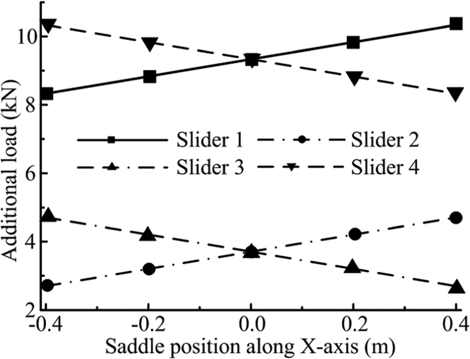
The variation in additional load of each slider.
According to related formulas (e.g. equations (22)–(24)) and parameter (such as Tables 1 and 2) in this article, we can calculate the equivalent stiffness and its variation in each slider–guide joint for different saddle positions, as shown in Figure 7.
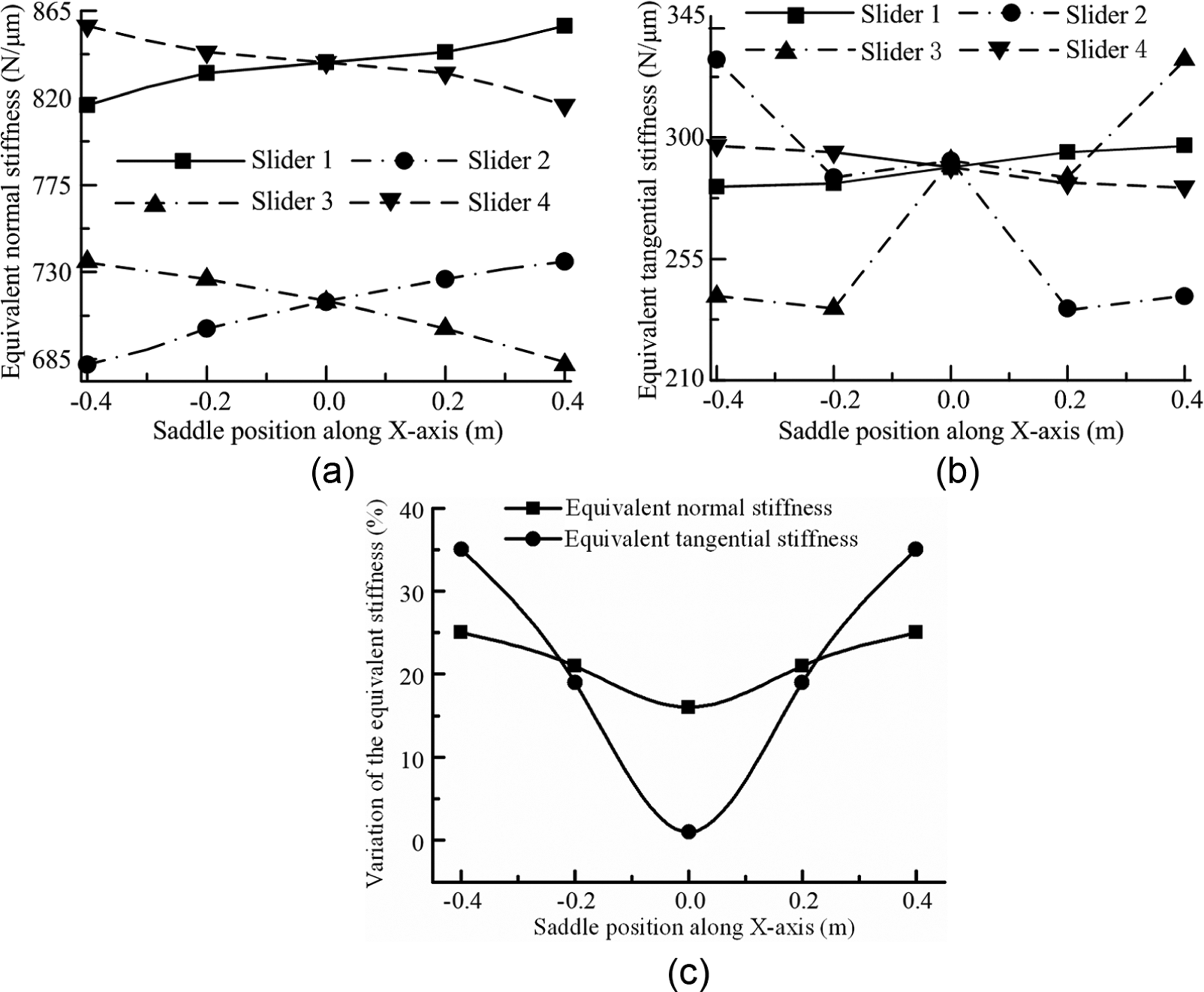
The variation in stiffness of each slider–guide joint: (a) equivalent normal stiffness, (b) equivalent tangential stiffness and (c) variation in the equivalent stiffness.
From Figure 7, we can see that the equivalent normal and tangential stiffnesses of each slider–guide joint change nonlinearly for different saddle positions. When the saddle is stationary, a maximal variation of 25% and 35% is found for the equivalent normal and tangential stiffnesses of the four slider–guide joints.
The traveling bridge system natural frequency
Figure 8 plots the acceleration vibration response for the test for different positions of the saddle (−0.4, 0.2, 0, 0.2 and 0.4 m). From the LMS Test.Lab, we can see that the mode shapes corresponding to the marked peak value of the response in Figure 8 are different, as shown in Figure 9.
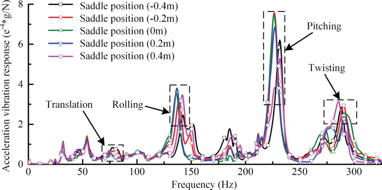
The experimental value of acceleration response for different saddle positions.
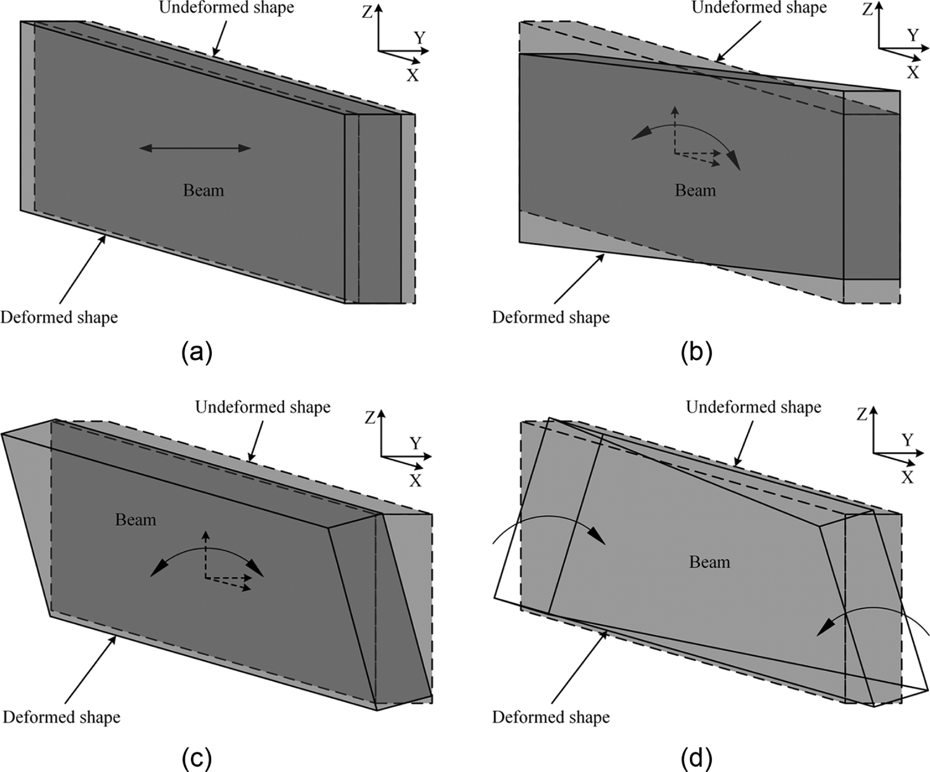
The typical mode shapes of the traveling bridge system: (a) translation, (b) rolling, (c) pitching and (d) twisting.
Based on the variable-coefficient dynamic equation, the related parameters and the variation in each slider–guide joint for different saddle positions in this article, we can obtain the frequency characteristics (fthe-vari) of the traveling bridge system for different saddle positions, as shown in Figure 10. In addition, the frequency characteristics (fthe-ideal) of the system were also calculated without considering the changes in stiffness for the slider–guide joints. The ideal normal and tangential stiffnesses of the slider–guide joints are 7.5 × 10⁸ N/m. The fexp in Figure 10 represent the experimental results (the marked peak value in Figure 8) of the traveling bridge system.
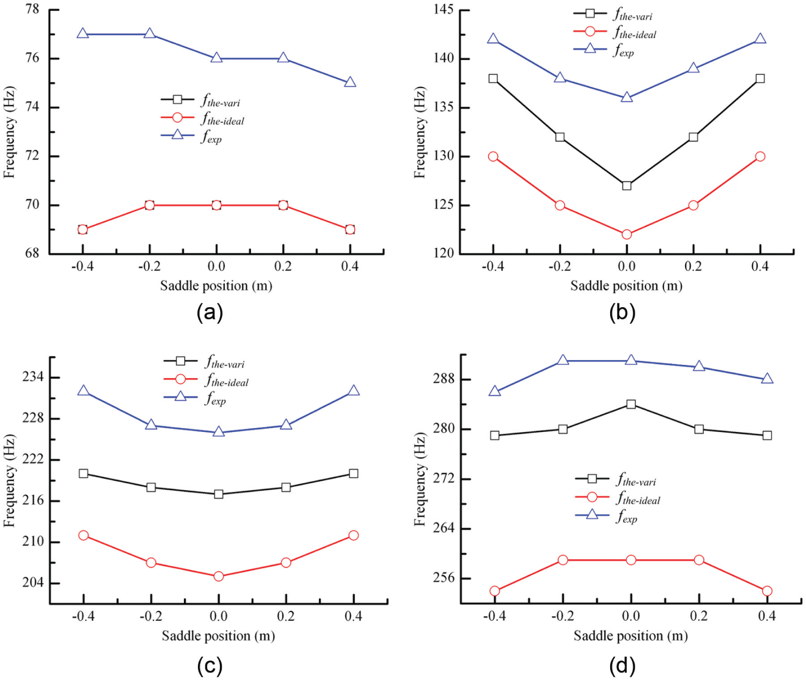
Comparison of the theoretical and experimental results: (a) translation, (b) rolling, (c) pitching and (d) twisting.
The equivalent normal and tangential stiffnesses of each slider–guide joint for different saddle positions are different; hence, the system stiffness matrix is also different for different saddle positions. On the other side, the system mass matrix is also different for different saddle positions. So, the solution (undamped natural frequency) of equation (1) is different when the damping matrix and the load matrix of the equation (1) are all 0. Therefore, the theory value of the undamped natural frequency for the gantry-type machine tools is different. In addition, we can think that the undamped natural frequency and the damped natural frequency (test values) are the same when we ignore the damping effect on the natural frequency.
From Figure 10(a), we can see that the fthe-vari value and the fthe-ideal value are the same under the same position. The reason is that this mode shape is mainly determined by the transmission stiffness of the Y-axis ball screw feed system and the transmission stiffness does not change with different saddle positions. From Figure 10(b), (c) and (d), it can be seen that the fthe-vari value is closer to the fexp value than the fthe-ideal value. The reason is that the fthe-vari value is considered the effect of axis coupling force on the slider–guide joints’ stiffness for different positions of the saddle. There are some errors between the theoretical calculation results and the experimental results for the natural frequency, and the main reason may be that the beam of the gantry-type machine tools is simplified as a beam element model, or the calculation value is not fit well with the actual value of the slider–guide joints’ stiffness. In a word, the dynamic modeling proposed in this article can reach a higher analysis accuracy. Besides, for analyzing the dynamics of the gantry-type machine tools, the modeling method in this article is faster than FEM that already exists in publications.
Conclusion
In this article, considering the effect of axis coupling force on the slider–guide joints’ stiffness, a variable-coefficient dynamic equation is proposed to depict the varying dynamics behavior for the gantry-type machine tools. The main conclusions of this article are as follows:
The additional load of the slide blocks supporting the beam varies with the position of the saddle, which would further affect the equivalent normal and tangential stiffnesses of the slider–guide joints. The stiffness of each slider–guide joint changes nonlinearly for different saddle positions. The difference in additional load reaches about four times among each slider, and a maximal variation of 25% and 35% is found for the equivalent normal and tangential stiffnesses of the four slider–guide joints when the saddle is stationary.
The frequencies of the traveling bridge systems of the gantry-type milling machine tools are analyzed. The theoretical calculation and experimental results all show that the variable-coefficient dynamic equation considering the effect of axis coupling force on the slider–guide joints’ stiffness can reach a higher analysis accuracy.
The traveling bridge systems’ frequencies of the gantry-type milling machine tools vary with the saddle position. Therefore, the traveling bridge systems possess position-dependent dynamics and the dynamics variation can provide guidance for active design and control of the CNC machine tools.
Footnotes
Appendix 1
Declaration of conflicting interests
The author(s) declared no potential conflicts of interest with respect to the research, authorship and/or publication of this article.
Funding
The author(s) disclosed receipt of the following financial support for the research and/or authorship of this article: This work was financially supported by the key project of National Natural Science Foundation of China (Grant No. 51235009).