
Abstract
An improved fuzzy-filtered neural network model is utilized to predict spindle deformation based on temperature data. The improved fuzzy-filtered neural network model combines the fuzzy logic qualitative approach and neural network adaptive capabilities, and it is composed of fuzzy filtering and adaptive layers. A verification experiment is conducted to evaluate the performance of the improved fuzzy-filtered neural network model. Nine Pt100 thermal resistances are employed to monitor spindle temperature. An inductive current sensor is utilized to detect spindle deformation. Experimental results show that the improved fuzzy-filtered neural network model can better predict spindle deformation than back propagation network, and it can significantly improve the performance of the spindle. Under the new cutting condition, the residual error of spindle deformation along the z-axis can be reduced to less than 6 µm.
Introduction
With the increasing demand for machining accuracy, manufacturers have been working on improving the performance of the components of main machine tools. Among all components of machine tools, the spindle is the key component because it provides the cutting motion to remove material and directly affects the accuracy of machine tools. Thus, the performance of spindles has a significant influence on the performance of machine tools and the flexibility of the production system. 1
The machining accuracy of machine tools depends on positioning errors. Thermal errors caused by internal heat sources and the environment reach up to 70% of the overall position errors. 2 Temperature variations can produce thermal expansion, which leads to relative displacement at the cutting point and can significantly influence on the spindle because it is close to the cutting point. Heat in the spindle is mainly produced by the friction of bearings supporting the spindle, 3 such friction directly conducts heat into the spindle structure and causes thermoelastic deformations and thermal drift. Thus, geometric inaccuracies occur in the workpiece.
Regardless of how well machine tools are designed, there is a limitation of accuracy that could be achieved. Errors cannot be fully eliminated by detailed design. In many situations, constructing a precise structure model for machine tools is difficult, labor-intensive, and costly. Easier methods utilize error compensation. 4 Effective compensation can result in workpieces with increased accuracy, even when medium precision machine tools are used. 5 Thermal error compensation has become a cost-effective method to improve the accuracy of machine tools.
Since the publication of two keynote papers, the first about thermal effects from Bryan, 6 and the second about error reduction and compensation of machine tools from Weck et al., 7 many studies on these areas have been conducted. Error compensation techniques are generally divided into direct and indirect compensation.7,8 Direct compensation approaches periodically measure thermal displacements between the tool and the workpiece. However, determining the accurate value of thermal deformation during the machining process is difficult. Given that the sensors are exposed to severe conditions, the acquired data are disturbed by noises. Such disturbance leads to the inaccuracy of the training model. By contrast, indirect compensation methods based on auxiliary values, such as temperature data, are easier and more convenient. By using physical or mathematical methods, researchers build relationship models between temperature data and thermal deformation. Various techniques, such as finite element analysis,9,10 grey system theory,11,12 regression analysis,13,14 neural networks,15,16 and combinations of two or three methods,17,18 have been developed.
Currently, most of studies focus on artificial neural networks (ANNs) to build thermal error predictive models based on selected important temperature data. Compared with other models, ANNs can be used to develop empirical models between discrete temperature data and thermal deformation and have the advantages of self-learning capability, parallel processing, and information distribution savings. Different types of ANNs, such as back propagation (BP) network, 19 radial basis function (RBF) network,16,20 grey neural network, 21 Elman network, 22 cerebellar model arithmetic computer (CMAC) neural network, 23 and integrated recurrent neural network, 24 have been developed for thermal error models in recent year. However, the working conditions of machine tools are generally complex and filled with unexpected noises. Researchers commonly mount many sensors on different positions to avoid missing key temperature points. However, this approach produces redundant information and increases complexity. Relying solely on neural modeling approaches does not guarantee the extraction of important information from redundant information and the appropriate elimination of unexpected noises. As such, a new model that can maintain balance between structural complexity and avoiding missing important information must be developed.
In this study, an improved fuzzy-filtered neural network (FFNN) model is developed. The model combines the fuzzy logic qualitative approach and neural network adaptive capabilities to predict spindle deformation. The proposed FFNN has better network structure flexibility and can more effectively approximate a highly nonlinear relationship than neural networks. Experiments are conducted on the spindle of a computer numerical control (CNC) machining center to evaluate the performance of the model. The results show that using the improved FFNN model can effectively predict spindle deformation. The predictive accuracy of the proposed network is higher than BP network.
The rest of this article is organized as follows. Section “Classic FFNNs” provides a brief description of the classic FFNN model. Section “The thermal error predictive model” presents the improved FFNN model. Section “Experimental setup” describes the experimental setup and measurement results. The experimental results and comparisons of the improved FFNN model and the BP network are presented in section “Results and discussion.” Final Section “Conclusion” presents the conclusions.
Classic FFNNs
Figure 1 shows the architecture of the classic FFNN model, where xi is the input and y is the output. 25 The nodes of the same layer have the same function.
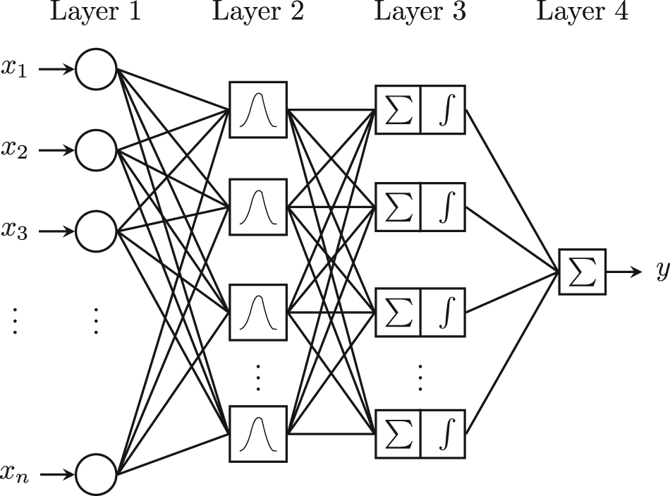
Classic fuzzy-filtered neural networks.
Layer 1 is the input layer that receives original data. Layer 2 is the fuzzy filtering layer. This layer merges and partitions the original data into fewer fuzzy channels to decrease the complexity of the system. The fuzzy channel defines a range of input intensities characterized by an appropriate membership function. Each node is connected to a generalized bell membership function expressed as follows
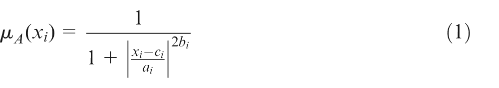
where xi denotes the position of the input channel, A is the linguistic term associated with this node function, and
where
Layer 3 is the perception layer. This layer that employs the same node function as the hidden layer has standard multilayer perception. Each node receives the weighted summation of inputs and produces a transferred output with a sigmoid function.
Layer 4 is the output layer. This layer computes the summation of incoming inputs from the previous layer. In this type of structure, the outputs depend not only on the fuzzy inputs but also on the intensity of the inputs.
The thermal error predictive model
Generally, each prediction stage has a direct relationship with one or a few dominant features of the previous stage in the dynamic system. Merging all features into each prediction stage is unnecessary. Redundant features can result in overfitting and may deteriorate the prediction results. To maintain the balance between structural complexity and avoiding missing important features, we need to build a prediction model that can extract the main features from a number of input channels and has the flexibility to adjust the network structure.
Improved FFNNs
Although classic FFNN can effectively partition large physical data channels into fewer fuzzy channels, the use of classic FFNN for high-speed applications, such as real-time forecasting, is difficult because the FFNN architecture is more complex than that of other neutral networks (especially in the consequent part), more time-consuming and more costly to solve. Moreover, classic FFNN lacks flexibility in certain aspects of the network structure and cannot effectively approximate a highly nonlinear relationship.
We improve the structure of classic FFNN to address the aforementioned difficulties. First, we simplified the fuzzy filtering part of classic FFNN and employed Gaussian functions as band-pass filters to process input data and speed up computation and avoid overfitting. In contrast with the generalized bell membership function of classic FFNN, the improved FFNN has fewer control parameters. Second, adaptive layers were added to the consequent part of classic FFNN to enhance the flexibility of the structure. Compared with classic FFNN, the improved FFNN does not have adaptive nodes. Based on these improvements, we applied the improved FFNN model, which is composed of fuzzy filtering and adaptive layers. Fuzzy filtering layers were used to filter noise, detect features, and partition a large number of physical data channels into fewer fuzzy channels. Adaptive layers were used to adjust the model structure.
The architecture of the improved FFNN model is shown in Figure 2. It consists of five layers that perform different actions. The output of the node of layer l is denoted as
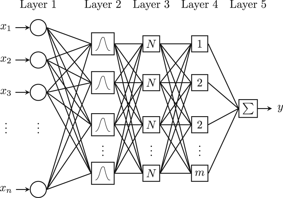
Improved fuzzy-filtered neural networks.
Layer 1 is the input layer that receives original data. Layer 2 is the fuzzy filtering layer. Gaussian functions were utilized as band-pass filters to process input data, which are expressed as follows
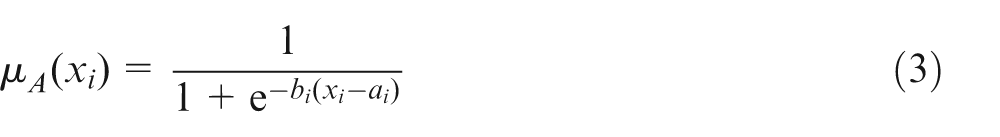
where A is the linguistic term associated with this node function, xi denotes the position of the input channel, and
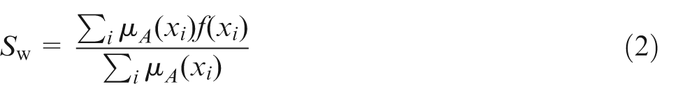
In this layer, all the incoming channels from Layer 1 are filtered. The output of Layer 2 can be calculated with the intensity functions, as follows
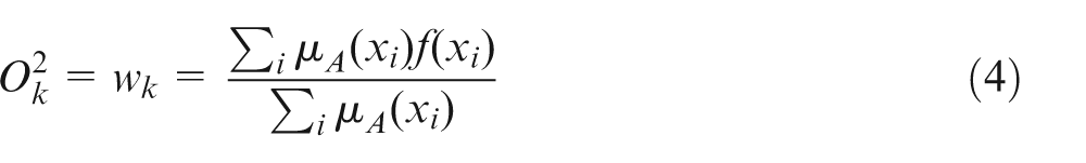
where
Layer 3 is the normalization layer. The nodes are fixed nodes labeled with N, indicating that they play a normalization role in the firing strengths of the previous layer. The outputs of this layer are expressed as
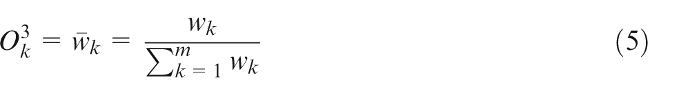
where m denotes the number of nodes in Layer 3.
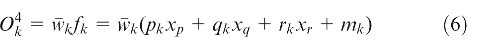
Layer 4 is the consequent layer with adaptive nodes. The output of each node is simply the product of the normalized firing strength
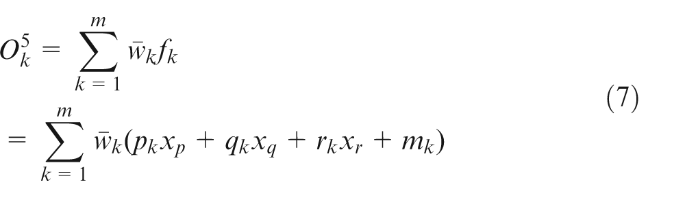
Layer 5 is the output layer. This layer is a single fixed node labeled with ∑. This node performs the summation of all incoming signals. Thus, the overall output of the model is expressed as
Fuzzy c-means clustering
In Layer 4, three central inputs, namely
The minimum of the following objective function was solved as
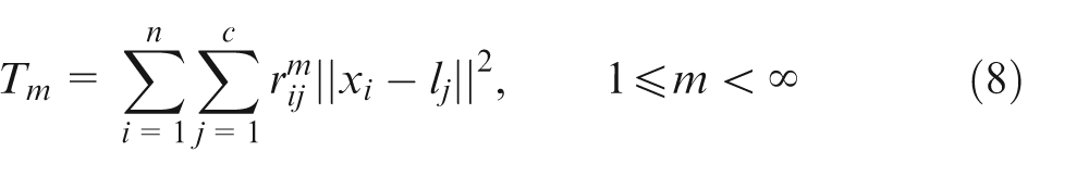
where m is any real number greater than 1,
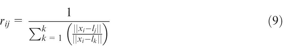
Fuzzy partitioning was implemented through iterative optimization of the objective function. The process is described below.
Step 1. Initialize matrix
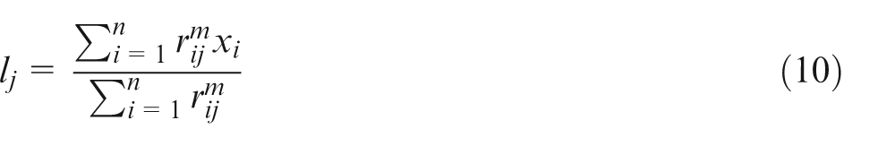
Step 2. Using equations (9) and (10), calculate the center vector
Step 3. If
Adaptive genetic algorithm
The genetic algorithm (GA) was employed to solve the improved FFNN model. GA is an evolutionary algorithm that optimizes problems by using techniques based on natural evolution, such as inheritance, mutation, selection, and crossover. GA is a powerful optimization tool and can be applied to many fields. However, GA has several problems that affect the efficiency of the solution. In the evolution process of GA, several individuals whose fitness is larger than that of other individuals may exist. These individuals are selected with high probabilities and induced prematurity. Moreover, a fixed parameter setting also results in premature convergence. Therefore, an adaptive GA was developed to solve the problem in the improved FFNN model.
The mean and standard deviation were utilized to derive the fitness function and obtain better fitness assignment. At the beginning of GA, all individuals are randomly distributed. The standard deviation of each generation is high. When GA is implemented, the standard deviation of individuals tends to decrease.
At the beginning of the algorithm, most of the individuals have not attained the optimal value. The difference in fitness between any two individuals should be small. At the end of the algorithm, the difference in fitness between good and bad chromosomes should be sufficiently large to ensure the convergence of GA. For the ith generation, fitness F can be adjusted by using the following equation
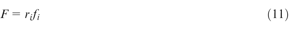
where ri denotes the adjusting coefficient for the ith generation and fi denotes the value of the objective function of each individual. With the progress of GA, ri changes accordingly, and fi becomes small. Adjusting coefficient ri is calculated as follows
where σi denotes the standard deviation of the ith generation.
Experimental setup
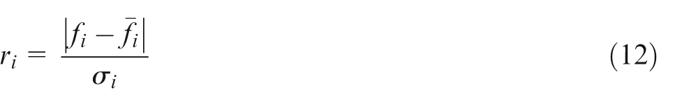
As shown in Figure 3, experimental setup is composed of a high-performance portal machining center, sensing units, and a data processing system. The machining center is a portal-type milling machine that has a movable cross rail (x-axis), worktable (y-axis), and ram (z-axis).The power of the spindle is 60 kW, the maximum speed is up to 3000 rpm, the repeatability accuracy is 0.003 mm, and the positioning accuracy is 0.01 mm.
Sectional view of the spindle.
Sensing units
The sensing units include nine Pt100 thermal resistances and an inductive current sensor. Pt100 thermal resistances were used to monitor the temperature variations of the spindle. The inductive current sensor was used to measure spindle deformation along the z-axis.
The main heat sources of the spindle are the support bearings. Owing to the friction torque between the rolling elements and the inner and outer raceways, the bearings generate a considerable amount of heat and have a significant influence on spindle deformation. The sensors were attached to these bearings. As shown in Figure 3, the spindle has three groups of bearings to support the mandrel. The bearings were arranged as follows: double-row roller bearing at the front of the spindle, face-to-face angular contact bearing at the middle of the spindle, and double-row roller bearing at the rear of the spindle. Nine Pt100 thermal resistances were attached to the three groups of bearings. Each group had three Pt100 thermal resistances uniformly arranged along the circumference. The inductive displacement sensor was installed on the worktable.
Data processing system
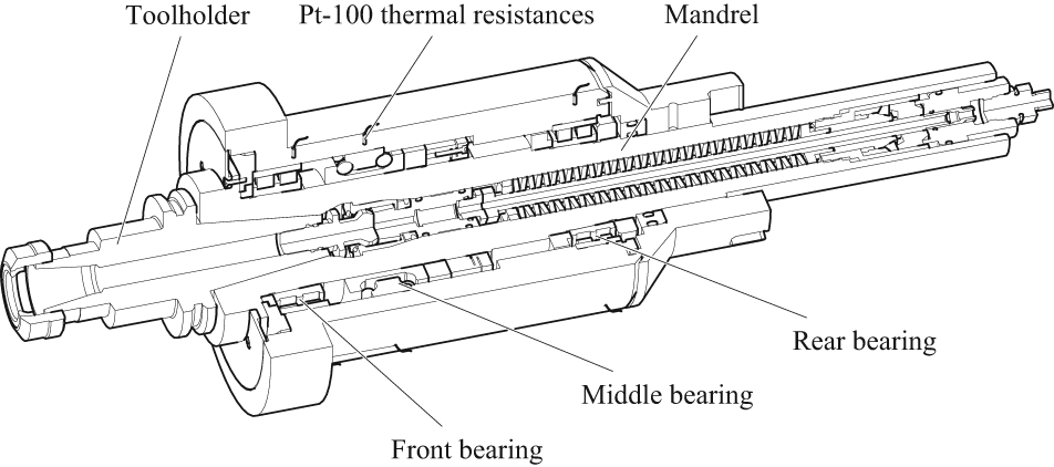
As shown in Figure 4, the data processing system is composed of a high-precision data acquisition card PXI-4351, a data acquisition system PXI-9230, and a personal computer (PC). The nine Pt100 thermal resistances and the inductive current sensor were sampled by PXI-4351. PXI-9230 was employed as the hardware processing platform because of its high processing speed and easy programming. By using LabVIEW, the data processing program was created to analyze the sampled data. The entire process was controlled by a PC.
Schematic illustration of experimental equipment.
Experimental conditions
The experimental datasets should be spread throughout the entire machining process, including warm-up, pause, and thermal equilibrium, to enhancing the robustness of our proposed model. The experiment was implemented to simulate the cycle of cutting a workpiece. The 300-min experiment time was divided into 300 intervals. Spindle deformation and temperature variations were recorded at a sampling interval of 1 min. At the end of each interval, spindle deformation was measured as the spindle moved on the inductive current sensor. The experimental data were divided into two groups: one for training and one for testing the model. At different spindle speeds (Figures 5(a) and 6(a)), we measured the temperature variations of the spindle and calculated three central temperature inputs through fuzzy c-means clustering, as shown in Figures 5(b) and 6(b), respectively. They are determined by the speed of the spindle in Figures 5(a) and 6(a). When the speed of the spindle increase or decrease, the temperature in Figures 5(b) and 6(b) also rise or descend. The blue (pink and cyan) line denotes the temperature change of the front (middle and rear) bearing under different speeds of the spindle. The thermal deformation of the spindle along the z-axis was measured, and the results are denoted by the blue line in Figures 5(c) and 6(c).
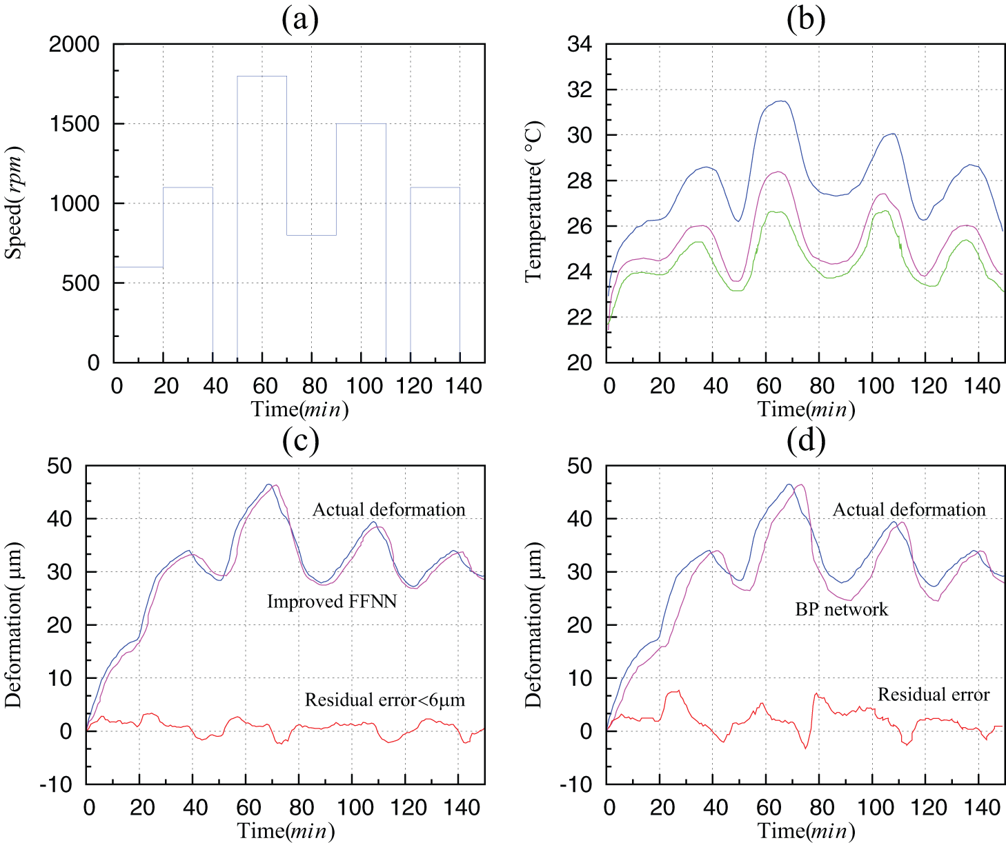
Training dataset (a) the spindle speed, (b) three central temperature inputs
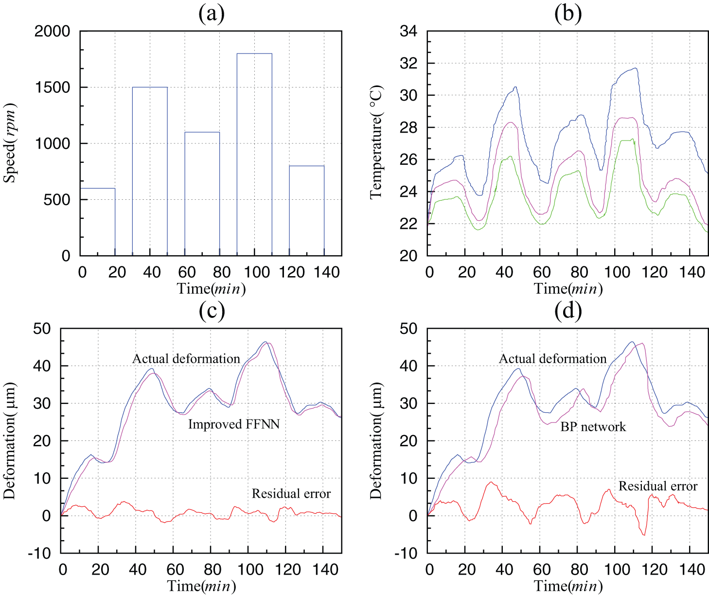
Testing dataset (a) the spindle speed, (b) three central temperature inputs
Results and discussion
The training dataset was utilized to train the improved FFNN model. During the training process of the improved FFNN model, the error of convergent criterion ε was set to 0.1 µm. Through the use of adaptive GA, the optimal parameters of the improved FFNN model were obtained. A comparison of the output of the improved FFNN model and the measured data on spindle deformation is shown in Figure 5(c).
The testing dataset was utilized to validate the effectiveness of the improved FFNN model. A comparison of the output of the improved FFNN model and the measured data on spindle deformation is shown in Figure 5(c). As shown in figure, the residual error of spindle deformation along the z-axis can be significantly reduced from 50 µm to less than 6 µm. The figure also shows that the improved FFNN model has good adaptability even under different conditions.
Comparisons with the BP network
The BP network, which has a topology structure of 8-16-1, was constructed to compare with different models. As shown in Figure 7, the BP network consists of input, hidden, and output layers. Nine input neurons receive temperature data from nine Pt100 thermal resistances, seven hidden neurons process the data with sigmoid functions, and one output neuron predicts spindle deformation along the z-axis. The learning rate was set as µ = 0.01, and the mean square error ε was set as 0.01.
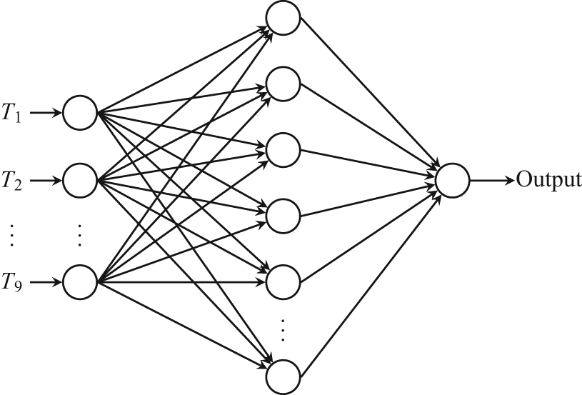
BP network architecture.
The following evaluation standards were adopted to compare the performances of the improved FFNN model and the BP network.
Root mean square error (RMSE)
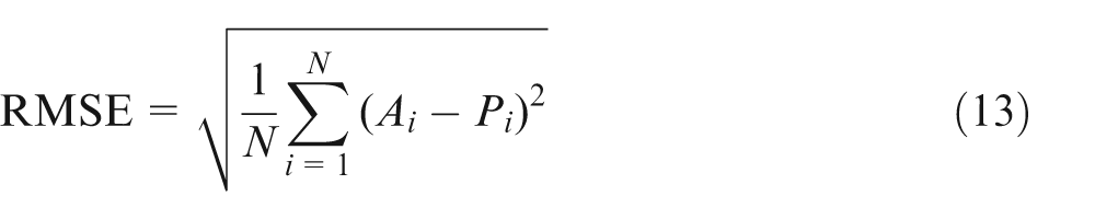
where Ai and Pi denote the actual and predicted deformation, respectively, and N denotes the number of datasets.
Mean absolute percentage error (MAPE)
Correlation coefficient (R)
where
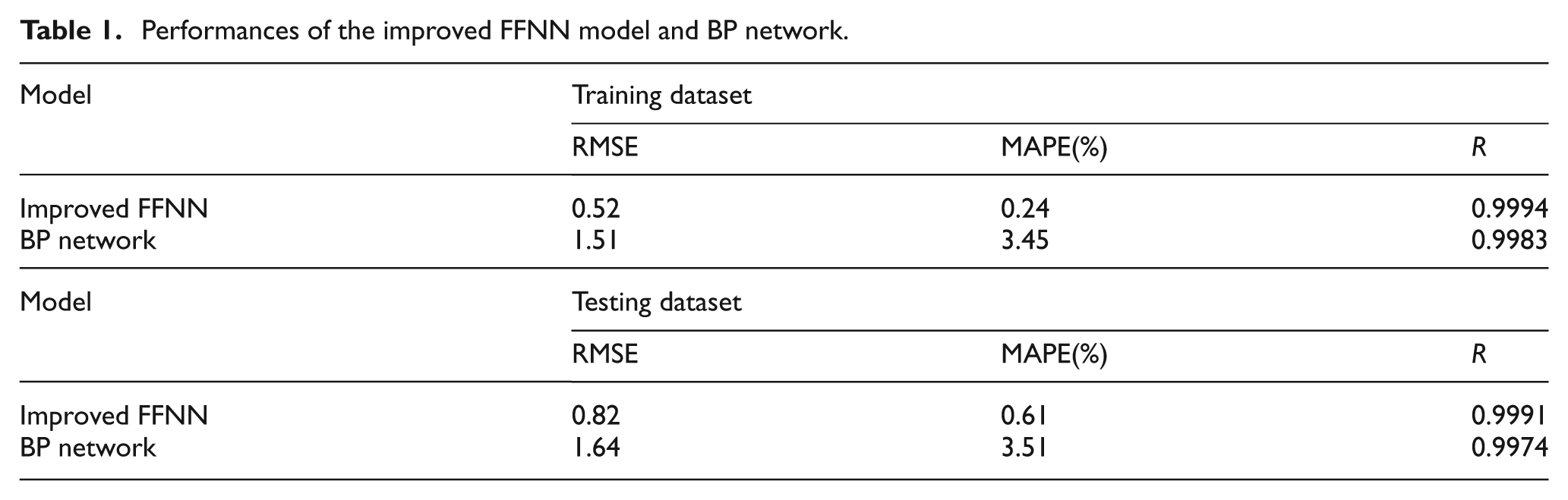
The performances of the improved FFNN model and the BP network are presented in Table 1. The improved FFNN model has a smaller RMSE and MAPE and a bigger R than the BP network.
Performances of the improved FFNN model and BP network.
The BP network was utilized to predict spindle deformation along the z-axis. The results of training and testing are shown in Figures 5(d) and 6(d), respectively. The BP network has a large deviation for actual spindle deformation during the warm-up stage. The BP network generates a good effect only when the temperature smoothly increases and the heat equilibrium of the spindle reaches a stable status.
The measured values of spindle deformation in intervals [35,50], [60,75], [100,115], and [130,145] are large because of the change in working conditions. The curve of these intervals is steeper than that of the other sampling points, as shown in Figure 5(c). The intervals shown in Figure 5(c) and (d) indicate that the improved FFNN model responds more quickly than the BP network. Thus, the improved FFNN model has a smaller residual error.
Conclusion
An improved FFNN model was developed to establish the relationship between temperature data and spindle deformation along the z-axis. The model is composed of fuzzy filtering and adaptive layers. The fuzzy filtering layers were used to filter noise and detect feature. The adaptive layers were utilized to adjust the model structure. The following conclusions were obtained.
With its fuzzy filtering layers, the improved FFNN model can effectively reduce the randomness of temperature data and the influence of unpredictable noises and can verify the importance of temperature data channels that directly affect the accuracy of the model. The improved FFNN model has better flexibility than the classic FFNN and can more effectively approximate a highly nonlinear relationship than neural networks because of the existence of adaptive layers.
An experimental validation was implemented. The experimental results showed that the improved FFNN model can precisely predict spindle deformation and significantly improve the thermal performance of the spindle. Under the new cutting condition, the residual error of spindle deformation along the z-axis can be reduced from 50 µm to less than 6 µm.
The comparison of the improved FFNN model and the BP network showed the superiority of the improved FFNN model in terms of predicting spindle deformation. Under the new cutting condition, the MAPE of the improved FFNN model is less than 0.7%, whereas the MAPE of the BP network is greater than 3%. The improved FFNN model responds more quickly than the BP network. Thus, the improved FFNN model has a smaller residual error.
Footnotes
Declaration of conflicting interests
The authors declare that there is no conflict of interest.
Funding
The work here is supported by the National Natural Science Foundation of China (No. 51175208, No. 51075161), the State Key Basic Research Program of China (No. 2011CB706803), and the Fundamental Research Funds for the Central Universities (No. 2013ZZGH001).