
Abstract
Thermal error is one of the major sources of machining inaccuracy. It becomes the dominant source of error and therefore should be predicted and compensated for. This article proposes a vector-angle-cosine hybrid model for thermal error prediction. The model combines the advantages of different constituent models and makes full use of the original measurement results. A multivariable linear regression model, a natural exponential model, and the finite element method are chosen as the three constituent models, and their advantages and disadvantages are demonstrated in detail. The combination weights of the three constituent models are determined by maximizing the cosine value of the angle between the vector-angle-cosine prediction vector and the actual thermal error vector. Experiments on spindle thermal errors are conducted to build and validate the proposed model. The performance comparison between the vector-angle-cosine hybrid model and the three constituent models indicates that the former has better accuracy and robustness under different working conditions. Some actual machining tests are conducted pre- and post compensation, and results show that the size errors are decreased by 60%.
Introduction
Researches indicate that thermal error accounts for 40%–70% of total errors on machine tools. Because machining accuracy is one of the most critical criteria for evaluating machine tools, the prediction and compensation of thermal error are highly important for improving the machining accuracy.
In recent decades, various researchers have focused on the development of thermal error models by using different modeling methodologies, such as artificial neural networks (ANNs), multiple linear regression (MLR) method, and finite element method (FEM). Yang and Ni 1 proposed an integrated recurrent ANN model to establish the spindle thermal error model. Kang et al. 2 presented a dynamic ANN model to predict thermal deformation in machine tools. Wu et al. 3 utilized the MLR method to predict the thermal errors of feed axes on a vertical machining center. Moreover, in research by Ni 4 and Zhu et al., 5 thermal deformation of the spindle was modeled using the MLR method. Some other thermal error prediction applications based on further development of the MLR method can also be found in three-axis or five-axis machine tools. For example, Chen and Hsu 6 proposed an autoregression dynamic thermal error model that considered the temperature history and the spindle speed information. Lin and Chang 7 developed a complex MLR analytical method to build a spindle thermal displacement model. The FEM has facilitated the in-depth analysis of the thermal behavior of machine tools under the influence of heat sources present inside the machine tool structure and its surroundings. 8 Zhao et al. 9 simulated the temperature field and thermal errors of the spindle under thermal loads. Creighton et al. 10 and Uhlmann and Hu 11 presented FEM models of high-speed motor spindles to predict the thermal behavior, and the results agreed well with the actual values. Wang et al. 12 developed an FEM model to predict the temperature distribution change and thermally induced errors of a crank press.
Besides the advantages of each model, its disadvantages should also be mentioned. The MLR is not suitable for highly nonlinear systems despite its simplicity in the mathematical format with high accuracy. The FEM lacks mathematical formats and simulation accuracy despite its suitability for mechanism analysis of thermal behaviors. If these advantages are effectively combined, hybrid models with higher prediction accuracy and better robustness can be obtained, as are listed below. Zhang et al. 13 proposed a gray neural network model, which combined the advantages of both the gray model and the neural network. Kang et al. 14 presented an accurate ANN model which combined three different filters to predict the thermal deformation in machine tools. Jedrzejewski et al. 15 built an effective hybrid model of a high-speed machining center headstock with integration of two sub-models modeled by FEM and finite difference method.
In this research, a vector-angle-cosine (VAC) hybrid model is proposed to predict the thermal errors caused by the heat generated in spindle. Section “Model descriptions” describes the three constituent models used in the VAC hybrid model. The principle and the algorithm of the VAC hybrid model are detailed in section “VAC hybrid model.” Section “Experiment for the spindle thermal error model building and validation” presents the experimental setup and thermal error measurement results, based on which the VAC hybrid model is built and validated. Finally, some conclusions are drawn in section “Conclusion and future work.”
Model descriptions
Before building the VAC hybrid model, an essential step is to pre-screen the constituent models. In addition to the models mentioned in section “Introduction,” there are also many other models for spindle thermal error prediction, such as natural exponential (NE) model, 10 harmonic analysis method, 16 and thermal mode analysis. 17 Here, MLR, the NE model, and the FEM are chosen to be the constituent models. The building process of the three constituent models is described as follows. The advantages and disadvantages are also demonstrated.
MLR and the least-square method
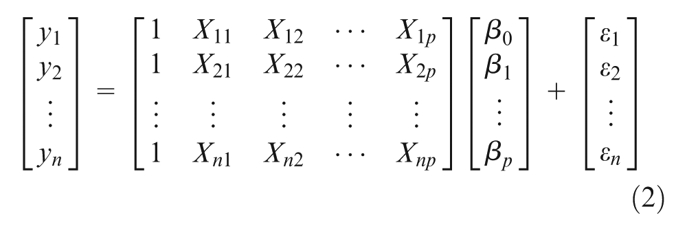
The generalized MLR model can be expressed by equation (1), with the number of independent variables as p

where β is the weight and ε is the corresponding error of the reaction variable y.
In the measurement, n sets of sample values are collected, and the matrix form can be used to write the general MLR model as the following equation
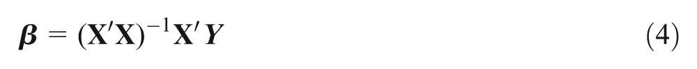
In short

It is assumed that an inverse matrix exists for matrix
From the perspective of the MLR method, the thermal error changes linearly with some key temperature variables, which reflect the thermal distribution of the machine tool. However, because of the complex interactions at the heat source location, different thermal resistance coefficients of machine components, and the cooling system’s liquid coolant effect, the machine tool thermal deformation process is highly nonlinear. Therefore, nonlinear modeling methods have attracted increasing attention in recent years.
NE model
The temperature of the spindle structure is related to the quantity of heat that flows into the spindle, Qin, and the quantity that flows out, Qout. The spindle is assumed to have a uniform structure and an initial temperature equal to that of the ambient surroundings.
When the quantity of heat, Qin, is generated step-wise at time t = 0, the temperature of the spindle can be expressed as follows 18
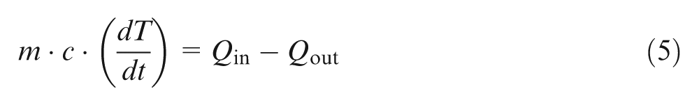

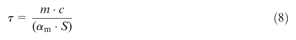
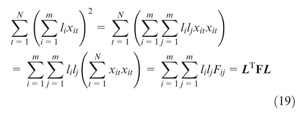
where m is the self-mass of the spindle; c is the specific heat of the spindle material; T and S are the temperature and the surface area of the spindle, respectively; and αm is the average heat transfer coefficient on the surface.
By solving equations (5) and (6) under steady-state conditions, the average temperature and the time constant of the spindle can be obtained as follows, respectively
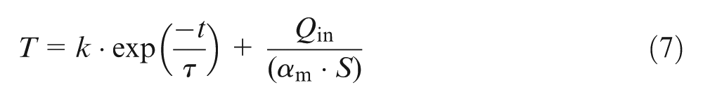
It can be easily found that the temperature model of the spindle is naturally exponential, so the model is called NE in this research.
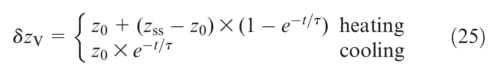
The axial deformation model of the spindle is described in equations (9) and (10) 10
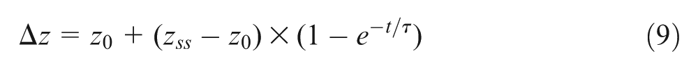

where Δz is the change in the spindle growth over time t, z0 is the spindle deformation at time 0, and zss is the steady-state spindle deformation for a particular speed.
There are two key points when building the model: first, the correct time constant τ has to be calculated, and second, the right relationship between zss and the spindle speed should be determined. The NE model mathematically demonstrates the mechanism of thermal behaviors and effectively represents the nonlinear system. However, the model is a function of time t, and not of temperature variables. There will be a tough problem of precisely calculating the time t, especially when short-term stops and restarts happen. So, it may lack robustness and accuracy.
FEM model
The spindle used in this research is shown in Figure 1. For this type of spindle, the most significant parameter affecting the thermal displacement is the friction heat in the front and rear bearings of the spindle. The heat produced by the spindle bearings is represented by equation (11) 19

where n is the rotating speed of the spindle (r/min) and M is the total frictional torque of the bearing (N/mm). The detailed process of calculating the parameter M can be found in Zhao et al. 9 and Harris. 19
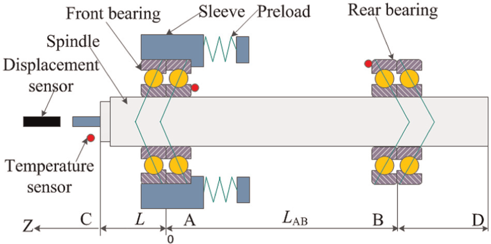
Schematic representation of spindle model.
There are two main types of heat transfer during spindle rotation, as shown in Figure 2. One is the heat conduction between the spindle and the bearings, and the other is the convection between the spindle and the ambient air. When the spindle is rotating, the convection is forced, whereas when the spindle stops rotating, the convection is natural.
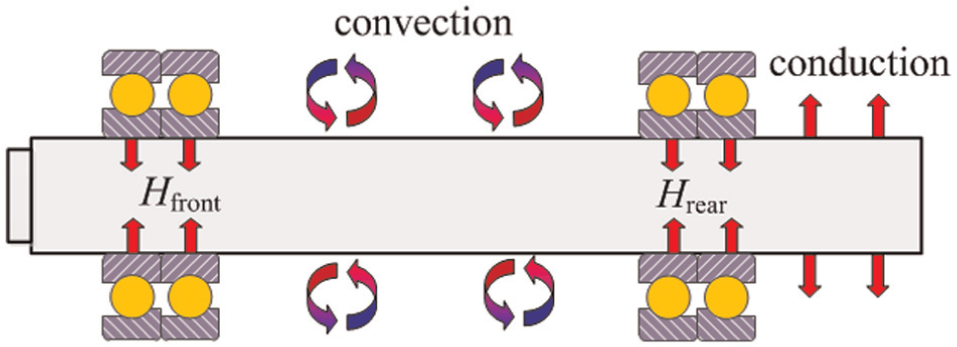
Heat transfer in spindle.
The coefficient of the forced convection heat transfer can be calculated using equation (12)
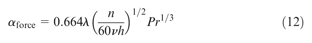
where λ is the thermal conductivity, ν is the kinematic viscosity of air (m2/s), h is a coefficient that is modified according to actual situations, and Pr is the Prandtl number of air. Under normal temperatures, the kinematic viscosity of air, v, equals 16 mm2/s, and the Prandtl number of air equals 0.701.
With the above boundary conditions, the temperature distribution and thermal deformation of the spindle can be obtained by the FEM. There are two main limitations of the FEM. One is the lack of access to the source code and the possibility of changing the way in which the solver operates. The other limitation is that the FEM programs do not ensure the required accuracy of modeling the thermal phenomena taking place in machine tools. 8
VAC hybrid model
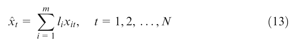
Let the thermal error series be xt, where t indicates the sampling time. In the hybrid prediction model, some constituent models are chosen to predict the thermal error first, and then combine those prediction values to output the final thermal error prediction value based on the VAC method. According to the weighted arithmetic mean principle for hybrid prediction, the VAC model can be defined as follows
where
As shown in equation (15),
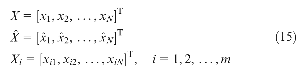
where N is the number of data sets during the tests and m is the number of constituent models.
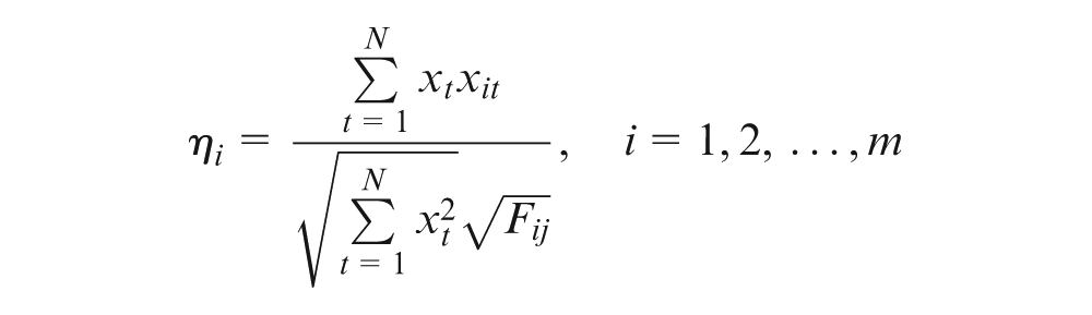
To describe the relationship between the above vectors, ηi is used to represent the cosine value of the angle between the vectors
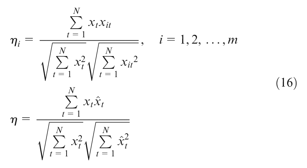
Let

where
Substituting equations (13), (17), (18), and (19) into equation (16), the following equations are obtained to calculate the values of ηi and η
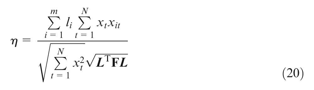
From equation (20), it can be clearly seen that the cosine value η is the function of combination weights, that is,
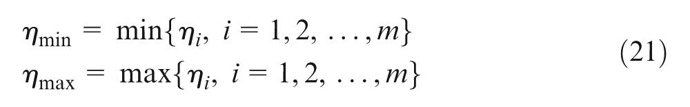
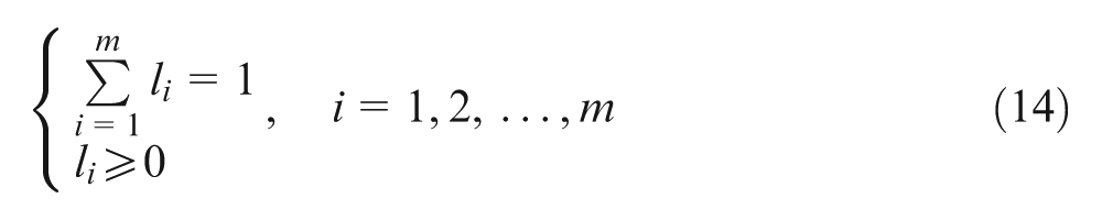
If
Based on the concepts described above, the combination weights of the VAC model can be determined by equation (22)
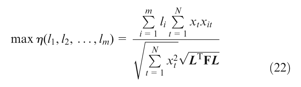

Equation (22) can be regarded as a nonlinear multivariable optimization problem, which can be solved using the MATLAB function fmincon().
Finally, the optimized weights for three constituent models are obtained from equation (22), and the VAC hybrid model is established. The algorithm flowchart of the VAC hybrid model is shown in Figure 3.
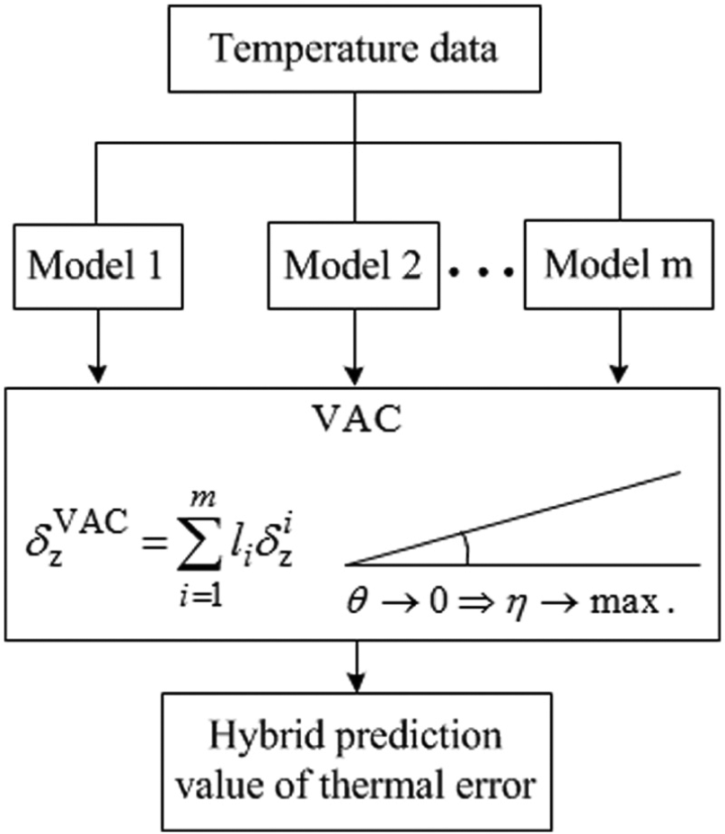
Algorithm flowchart of the VAC hybrid model.
Experiment for the spindle thermal error model building and validation
Experimental setup
The error components in the spindle motion have 6 degrees of freedom (DOFs), that is, 1 axial error, 2 radial errors, 2 tilting errors, and 1 angular positioning error. Here, the process of model building and validation for the axial thermal error δz is used as an example to illustrate the principle and effectiveness of the VAC hybrid model. Other DOF error components can be simultaneously modeled using the same method. Figure 4 shows the experimental setup for the temperature sensors. Because the front bearing, rear bearing and the ambient temperature influence the spindle thermal error most, T1, T2, and T3 are chosen as the key measuring points. Thermal errors in other directions can be modeled in the same way, without the computational details described in this article.
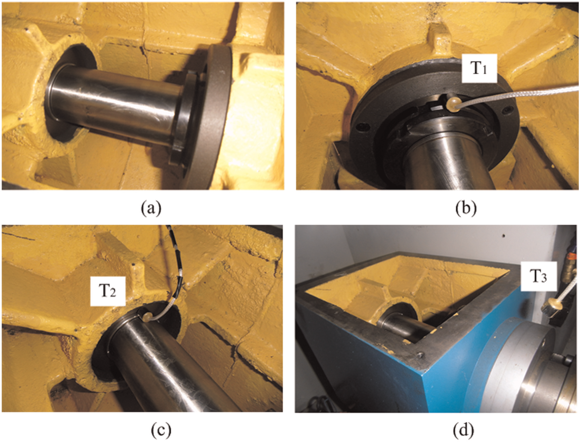
Locations of temperature sensors on spindle: (a) spindle appearance, (b) T1 at front bearing, (c) T2 at rear bearing, and (d) T3 at ambient air.
To examine the robustness of the proposed thermal error model, two measuring tests were conducted. The measurement data of the first test, shown in Figure 5(a), were used to build the thermal error model, whereas those of the second one, shown in Figure 5(b), were used to validate the model. During the tests, temperature variations at the three key measuring points and axial thermal errors were recorded under different speed spectrums.
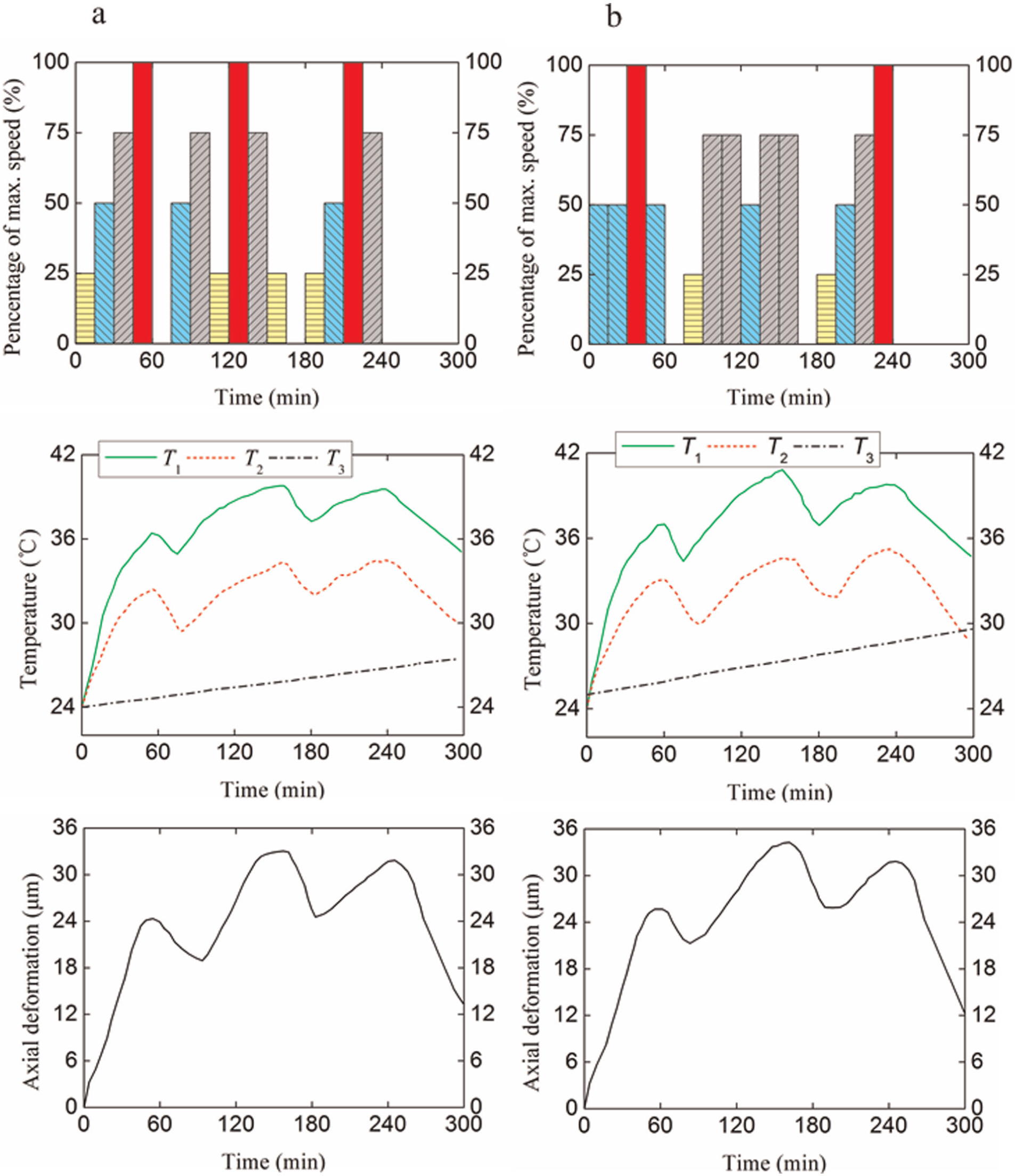
Measurements of spindle speed spectrum, temperature variations, and axial thermal error: (a) the first measuring test for modeling and (b) the second measuring test for validation.
According to ISO 230-3:2007, 20 all transducer outputs are monitored for a period of 4 h, and the spindle is stopped for a period of 1 h while the monitoring of the transducers is continued. This is because the effects of the test mandrel run-out should be eliminated during the tests when the spindle is rotating. The thermal errors were measured and recorded at a sampling interval of 4 min and included 76 data sets. All the experiments are repeated three times, and the average value is used to build the model.
VAC hybrid model building
Based on the measured data shown in Figure 5(a), the three constituent models can be obtained through the steps described in section “Model descriptions.”
Model 1
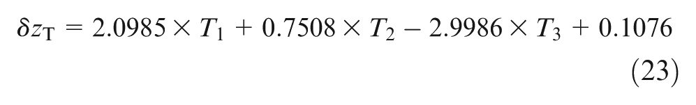
The MLR model is described by equation (23)
Model 2
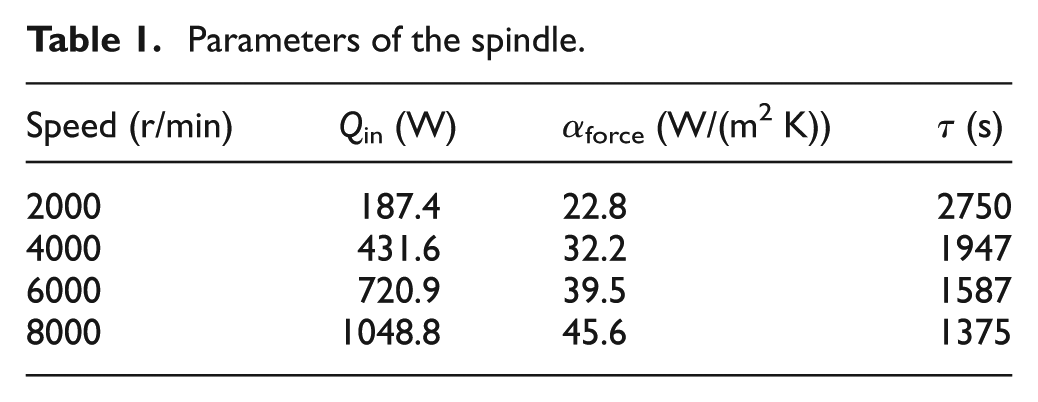
Some essential parameters for the NE model are listed in Table 1, and the time constant τ can be calculated by equation (8).
Parameters of the spindle.
The relationship between zss and the spindle speed can be obtained by experiments or the FEM. Here, the results from the FEM are used. The FEM results are shown in Figure 6, and the relationship is expressed by equation (24)

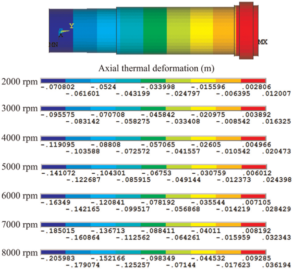
Nephogram of axial deformation under different speeds.
Based on equations (9), (23), and (24), the NE model is determined.
Model 3
The boundary conditions for the FEM model are listed in Table 1. The thermal deformation of the spindle in different directions can be obtained via ANSYS. Figure 6 shows the nephogram of steady-state axial deformation under different speeds. The transient deformation of the spindle can also be obtained via ANSYS by setting the correct boundary conditions. During the transient simulation, short-term stops are added. The deformation
The prediction values of three constituent models are listed in Table 2. These values are used to build the VAC hybrid model.
Prediction values of three constituent models (µm).
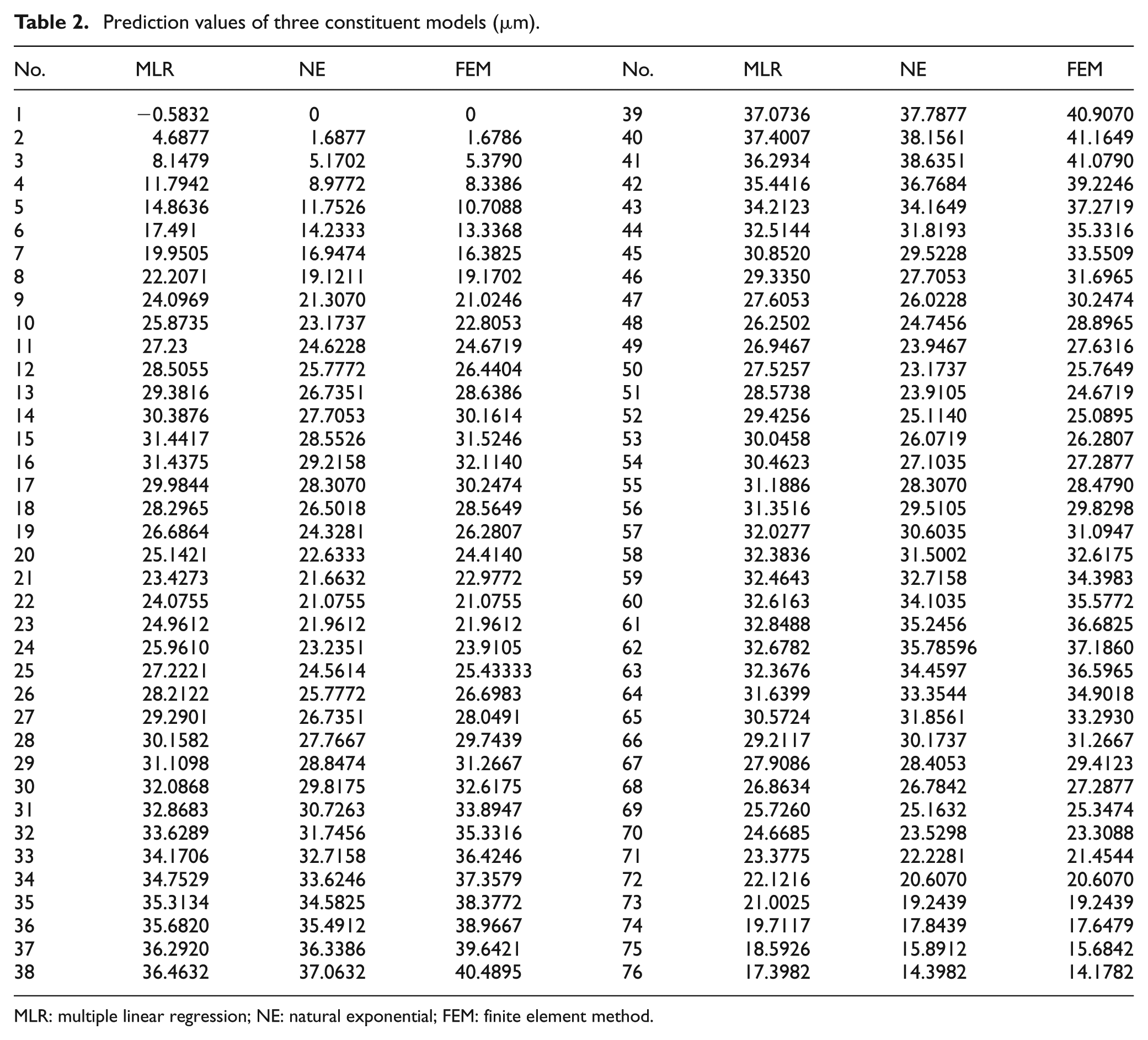
MLR: multiple linear regression; NE: natural exponential; FEM: finite element method.
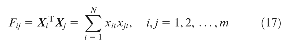
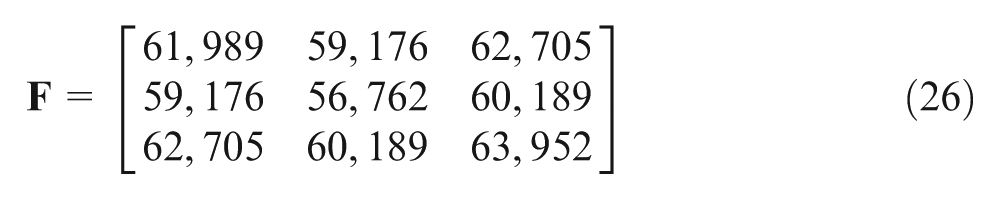
From equations (17) and (18), the information matrix of the VAC hybrid model can be obtained
The VAC prediction value can be calculated by combining the three constituent prediction values shown as follows

where
The optimization problem is solved using MATLAB, and the optimized weights for the three constituent models are as follows

Consequently, the model of spindle axial deformation is established. Using the same modeling method, the model of radial deformation can also be obtained.
Model validation and comparison
The second measuring test, shown in Figure 5(b), was conducted to further verify the robustness of the derived VAC model. All the constituent models used in the second test have the same structure and parameters as in the first test. The actual thermal error and the model prediction are shown in Figure 7. The VAC hybrid model clearly shows better accuracy and robustness than the constituent models. In addition, another three model evaluation indexes, that is, the sum of squareness of the error (SSE), the mean absolute error (MAE), and the mean absolute percentage error (MAPE) are used for comparing the performance of different models. The SSE, MAE, and MAPE are defined by equations (30)–(32). The comparison results listed in Table 3 indicate that the VAC hybrid model performs better than any of the constituent models
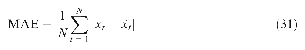

Model validation results: (a) MLR, (b) NE, (c) FEM, and (d) VAC.
Comparison of prediction models.
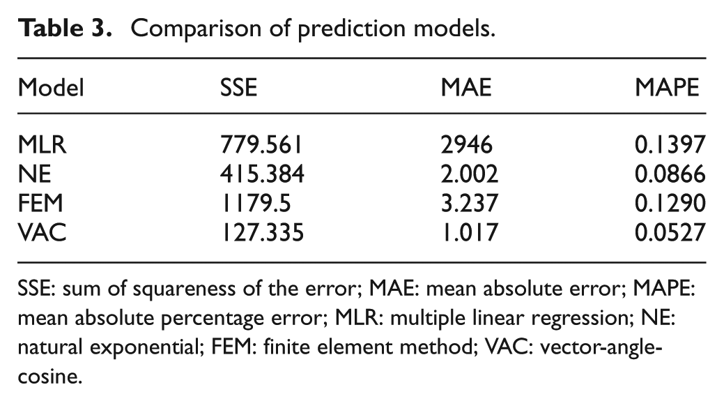
SSE: sum of squareness of the error; MAE: mean absolute error; MAPE: mean absolute percentage error; MLR: multiple linear regression; NE: natural exponential; FEM: finite element method; VAC: vector-angle-cosine.
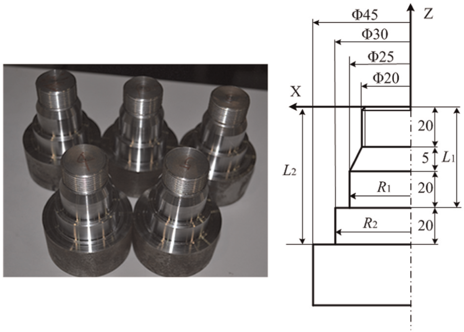
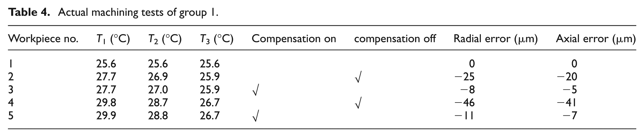
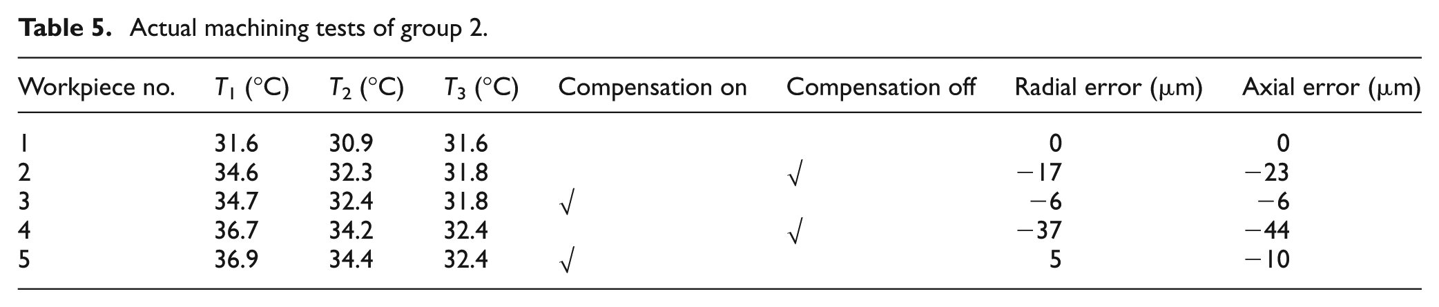
According to ISO 230-7:2006, 21 the spindle axial and radial deformations are simultaneously measured using a mandrel. The combination weights for radial thermal errors are calculated separately using the same method mentioned above. Some actual machining tests are conducted to validate the proposed model. The machine tool is used to cut two groups of workpieces under different temperatures. Each group has five workpieces, as shown in Figure 8. Radial size R and length size L are measured after machining, and the first workpiece is set as the reference, whose size errors of R and L are 0. The radial error and axial error of the workpieces are measured pre- and post compensation and are listed in Tables 4 and 5. The results show that size errors of the workpieces are reduced by 60%. The proposed model is effective for thermal error prediction.
Actual machining tests.
Actual machining tests of group 1.
Actual machining tests of group 2.
Conclusion and future work
Experimental results show that the proposed VAC hybrid model is effective for thermal error prediction and compensation on machine tools. The following conclusions can be drawn:
The VAC is an effective strategy for combined prediction. The optimized weights of different constituents can be determined by maximizing the cosine value of the angle between the VAC prediction vector and the actual thermal error vector.
The VAC hybrid model combines the advantages of different constituent models, and hence achieves higher prediction accuracy and better robustness. The VAC model is a good choice, especially when it is unknown which constituent model is more appropriate for thermal error prediction.
Data analysis of the thermal error measuring experiment reveals a nonlinear relationship between the thermal error and the temperature variables. Thus, the models with the nonlinear characteristic are more suitable for thermal error prediction than the linear models.
The VAC hybrid model has better accuracy and robustness than the other three constituent models. In the actual machining tests, the size errors of the machined workpieces are reduced by 60%, which validates the effectiveness of the VAC hybrid model.
Besides the advantages of the VAC hybrid model, if the weights of the three constituent models can be self-adjusted according to different machining conditions, a better prediction model can be obtained. In addition, whether or not the VAC hybrid model can be applied to motorized spindle and the screw is a problem worth considering.
Footnotes
Appendix 1
Declaration of conflicting interests
The authors declare that there is no conflict of interest.
Funding
This research was sponsored by the Specialized Research Fund for the Doctoral Program of High Education (No. 20110073110041), the National Science Foundation Projects of P.R. China (No. 51275305, 51175343), and the Chinese National Science and Technology Key Special Projects (No. 2011ZX04015-031).