Multi-objective vehicle routing problem with time windows: Improving customer satisfaction by considering gap time

Abstract

The vehicle routing problem with time windows is a combinatorial optimisation problem in distribution logistics. It has been infrequently measured as a multi-objective optimisation problem for the benefit of customers. For the purposes of this research, the measurement of multi-objective vehicle routing problem with time windows will be in terms of a minimisation of the total distance travelled by all vehicles, the total number of vehicles used (management beneficial objectives) and the total gap between ready time and issuing time (customer beneficial objective). It is possible to satisfy customers by issuing the goods as close as possible to the customer ready time. This is because possibilities for going out of stock during the above said time gap (by chance of improper inventory maintenance) are reduced with a minimised total time gap, which in turn increases the sales orders for the manufacturing management. An improved genetic algorithm, called the fitness aggregated genetic algorithm, has been implemented to resolve the problem. The proposed algorithm incorporates a fitness aggregation approach and dedicated operators, such as selection based on aggregate fitness value and best cost route crossover, to resolve the multi-objective problem. The algorithm was validated on Solomon’s bi-objective benchmark models for the minimisation of the total distance travelled and total number of vehicles used, and the results formed by proposed algorithm are competitive to best known results. After validating the proposed algorithm on bi-objective models, the third objective – namely, the total time gap between ready time and issuing time – is included in the bi-objective model. The results show that the suggested algorithm creates improved customer-satisfied routes without drastically affecting the total distance travelled and total number of vehicles used.

Introduction

The transportation of raw materials and completed products is an imperative duty for manufacturing industries, and massive funds are presently expended to accomplish this objective. The vehicle routing problem (VRP) is a transportation problem in the field of distribution, operations research and manufacturing management. The VRP is a non-deterministic polynomial-time hard (NP-hard) problem. The truth that VRP is both of analytical and realistic interest clarifies the amount of focus given to the VRP by researchers over the past years. ¹ The VRP can be described as the procedure of computing inexpensive routes for distribution vehicles to carry the necessary products to every single customer with the constraints that each vehicle has to begin and end at the central depot, each customer should be visited by one vehicle precisely and the sum of all customer demand in a route should not surpass vehicle capacity. ² The vehicle routing problem with time windows (VRPTW) is a variant of VRP. ³ In VRPTW, each customer has time windows and, in addition to the above constraints, all customers should be delivered within the time windows. However, vehicles might reach their destination before the time window opens, but the customer cannot be served until the time window opens and the vehicle should wait until the time window opens. The vehicle is not permitted to reach its destination after the time window has closed. ⁴ Although a group of research has already used single-objective optimisation with minimisation of the total distance travelled or cost to solve the VRPTW, it has not commonly been considered as a multi-objective optimisation problem due to the following reasons: the computation of non-dominated results is a solid procedure where the number of objectives raises and the amount of non-dominated results raises exponentially with the number of objectives. ⁵ But in the real world, the greater part of these routing problems has numerous objectives. Moreover, these objectives may not always be limited to the total distance or cost. In reality, many other aspects, such as the number of vehicles, the balancing of workloads (distance, load), waiting time and customer satisfaction among others, can be considered into account just by adding new objectives. ⁶ The use of multi-objective optimisation in routing problems attracts more researchers because it provides novel opportunities for defining problems. The following section provides a detailed literature survey of multi-objective routing problems.

Literature review

Ombuki et al. ⁷ have developed VRPTW as a bi-objective problem by considering the minimisation of the total distance travelled and number of vehicles. Here, a genetic algorithm (GA) with a Pareto ranking system was initiated for problem solving. The algorithm formed a set of impartial results for both objectives in the face of a huge number of typical benchmark cases. Tan et al. ⁸ have developed a bi-objective model for VRPTW, where the total distance travelled by all vehicles and the total number of vehicles used are considered as multi-objectives. Hybrid multi-objective evolutionary algorithm (HMOEA) was recommended for problem solving. The HMOEA incorporated local search exploitation with Pareto optimality and utilised particular genetic operators like route exchange crossover and multimode mutation. The HMOEA was then applied to solve Solomon’s benchmark instances, which gives 20 results superior to or as competitive as those evaluated to give the best known (BK) results. Jozefowiez et al.^9,10 presented a model for the bi-objective capacitated vehicle routing problem (CVRP), where minimisation of the total distance and route balance are the bi-objectives. They applied a multi-objective genetic algorithm (MOGA) with a target-aiming Pareto search and multi-objective evolutionary algorithm (MOEA) with elitist diversification method to solve the problem. The results show that the applied methodologies were fairly successful compared to other heuristics. Borgulya ¹¹ considered bi-objective CVRP, where the total distance travelled and route balance are minimised. MOEA with the extended virtual loser method was initiated to solve the bi-objective problem. The results prove the competitiveness of the suggested method in comparison with other evolutionary techniques. Ghoseiri and Ghannadpour ¹² developed a bi-objective VRPTW, where the minimisation of the total distance travelled and the number of vehicles used are the bi-objectives. They applied GA with goal programming method for problem formulation to solve the problem. The algorithm was validated for a large number of Solomon’s benchmark cases, with the results proving the efficiency of the algorithm introduced.

Muller ¹³ derived bi-objective VRP with soft time window, which involves the introduction of a penalty for abuse of the time window. Total cost minimisation (the sum of costs for the distance travelled and the number of vehicles used) and total penalty cost minimisation were thus measured as the objectives. Here, a heuristic technique was implemented to resolve this problem. The investigational results show that the beginning of the penalty plan leads to crucial savings in the total cost in certain cases. Chand et al. ¹⁴ reported a bi-objective VRPTW with the minimisation of the total distance and the number of vehicles. A MOGA with best cost route crossover (BCRC) and swap mutation (SM) was used here to solve the problem, while the results show the ability of the algorithm to determine the optimum solution effectively. Minocha and Tripathi ¹⁵ presented a model for bi-objective VRPTW, in which the total distance travelled and the number of vehicles used were minimised. They apply GA with local search heuristics (replacing next neighbour and reinserting random customer) to solve the problem. The results prove that the inclusion of local search heuristics enhances the efficiency of GA. Nahum et al. ¹⁶ derived a model for bi-objective VRPTW, in which the total distance travelled and the number of vehicles used were considered as bi-objectives. An artificial bee colony algorithm with vector evaluated approach was proposed to solve the problem. The results show that the algorithm is superior to the existing heuristics techniques. Chiang and Hsu ¹⁷ described bi-objective VRPTW by considering the minimisation of the total distance travelled and the total number of vehicles used. An evolutionary algorithm with knowledge-based genetic operators was then introduced for problem solving. The results produced were compared with the 10 existing algorithms proving the competitive performance of the algorithm introduced. Melian-Batista et al. ¹⁸ considered bi-objective VRPTW in which the total distance travelled and the route balance were minimised. A scatter search was proposed to solve the bi-objective problem. The algorithm was experimented upon Solomon’s benchmark instances and also tested on the real case of the Tenerife Company, Spain. The results coming from the proposed algorithm are competitive with the BK solutions and improve the solution implemented by the company.

Tan et al. ¹⁹ developed a new variant of VRP that integrates vehicle routing problem with stochastic demand (VRPSD), where the actual demand for a product is exposed only when the vehicle reaches the customer. The minimisation of travelled distance, the number of vehicles used and driver remuneration based on working hours were the multiple objectives of this VRPSD model. MOEA with local exploitation heuristic and route simulation method was then introduced to resolve the multi-objective VRPSD model. The results show the robustness of the algorithm in the face of the probabilistic nature of the problem. Hassan-Pour et al. ²⁰ introduced stochastic location-routing problem in which minimisation of facilities establishing cost and transportation cost and maximisation of the probability of delivery to customers were the multiple objectives. The problem was resolved in two stages by first solving the facility location problem using mathematical algorithm. Then, the multi-objective multi-depot VRP was solved using a hybrid algorithm which incorporates simulated annealing and GA. The results show the effectiveness of the suggested approach. Munoz-Zavala et al. ²¹ reported multi-objective VRPTW with minimisation of the total distance, number of vehicles and total waiting time. Particle swarm optimisation algorithm with space partitioning was initiated to solve the multi-objective problem, and the results prove the importance of space partitioning to determine the non-dominated solutions. Najera and Bullinaria ²² presented a multi-objective VRPTW, where the total distance travelled, total delivery time and the number of vehicles used were the multi-objectives. An MOEA with similarity measurement technique was proposed to solve the problem. The results prove that the implementation of the similarity measurement technique ensures the excellence of results.

Chand and Mohanty ²³ considered multi-objective VRPTW with the minimisation of the total distance, the number of vehicles and time window violation. A MOGA with BCRC and exchange mutation was used to resolve the problem, and the results show the capability of the algorithm to determine the optimum solution effectively. Banos et al.^24,25 derived a multi-objective VRPTW, minimising the total distance travelled and workload imbalance in terms of distance and load. They initiated hybrid algorithm (evolutionary computation and simulated annealing) and the multiple temperature Pareto simulated annealing algorithm. The computational results show the enhanced performance of the recommended algorithms. Konstantinidis et al. ²⁶ developed a multi-objective VRPTW, where the minimisation of the total distance, the number of vehicles and the route balance were the multiple objectives. Multi-objective evolutionary algorithm with decomposition (MOEA/D) was implemented to solve the tri-objective problem, and the results prove the better performance of MOEA/D against MOEA. Sivaramkumar et al. ²⁷ developed multi-objective VRPTW in which the minimisation of the total distance travelled, the total number of vehicles used and the route balance were the multi-objectives. Here, a GA with the BCRC and SM was proposed to solve the multi-objective problem. The proposed algorithm was experimented on Solomon’s benchmark problems, and the results show the ability of the algorithm to determine the better route-balanced solutions without radically disturbing the total distance travelled and total number of vehicles used. Molina et al. ²⁸ introduced VRP with a new combination of multiple objectives, namely, minimisation of internal costs, carbon dioxide emissions and nitrogen oxide emissions. An algorithm based on savings heuristics was proposed here to solve the problem. A real-life case application to a leading food distributing company in Spain was then examined to verify the realism of the introduced model and the suggested algorithm.

Tables 1 and 2 give a summary of and comments upon the literature survey based on a combination of multi-objectives and problem solving, respectively. From the above survey and summary, it is inferred that although multi-objective routing problems have frequently been considered in recent years, much of the work is focused only on the management beneficial side and ignores customers’ desires. Similarly, real-life industry problems are rarely been measured for problem solving. Our research is an attempt to overcome the first gap in research by considering multi-objective routing problems that are beneficial to both management and customers. In view of the need to give due consideration to customer satisfaction, management may initially lose a smaller quantity of its optimal inputs (distance, vehicles, etc.) by deriving a multi-objective model with customer welfare. However, in the long run, the proportionate raise in outputs (customer’s network, turnover, goodwill, continuous improvement, etc.) will visibly control the proportionate rise in optimal inputs. Benefits to customers may be given in the following ways: timely delivery, discounts for large orders and buy back of the unsold products. However, giving benefits without any additional cost is possible only by means of timely delivery. In VRPTW, each customer has time windows within which the products must be issued. Each time window has a ready time and a due time. The ready time is the time at which the window opens; only after that can the goods be issued to the customers. Due time is the time at which the window closes; before that the goods should be delivered to the customers. It is possible to satisfy customers by issuing the goods as close as possible to the customer ready time. The advantage is that the possibilities of being out of stock (by chance of improper inventory maintenance) are reduced by issuing the goods as close as possible to ready time. To achieve this, a new parameter – namely, ‘gap time’– is introduced in this article. Gap time is the difference between ready time and goods issuing time. By minimising the gap time, it is possible to deliver the goods as close as possible to the ready time. Hence, customer satisfaction can be improved which, in turn, helps management to retain customers for future orders and bulk orders. For this research, multi-objective VRPTW is measured in terms of the minimisation of the total distance travelled by all vehicles, the total number of vehicles used (management beneficial objectives) and the total gap time (customer beneficial objective).

Table 1.

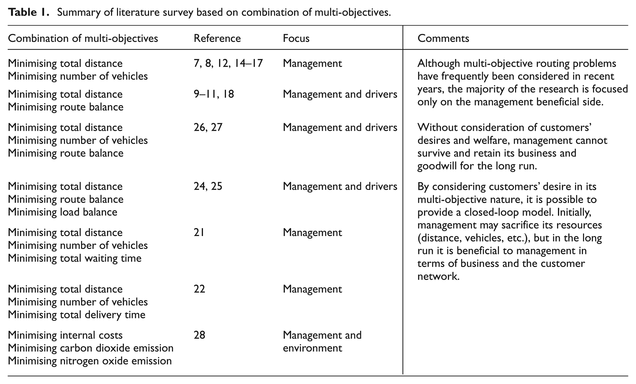
Summary of literature survey based on combination of multi-objectives.

Combination of multi-objectives	Reference	Focus	Comments
Minimising total distance	7, 8, 12, 14–17	Management	Although multi-objective routing problems have frequently been considered in recent years, the majority of the research is focused only on the management beneficial side.
Minimising number of vehicles
Minimising total distance	9–11, 18	Management and drivers
Minimising route balance
Minimising total distance	26, 27	Management and drivers	Without consideration of customers’ desires and welfare, management cannot survive and retain its business and goodwill for the long run.
Minimising number of vehicles
Minimising route balance
Minimising total distance	24, 25	Management and drivers	By considering customers’ desire in its multi-objective nature, it is possible to provide a closed-loop model. Initially, management may sacrifice its resources (distance, vehicles, etc.), but in the long run it is beneficial to management in terms of business and the customer network.
Minimising route balance
Minimising load balance
Minimising total distance	21	Management
Minimising number of vehicles
Minimising total waiting time
Minimising total distance	22	Management
Minimising number of vehicles
Minimising total delivery time
Minimising internal costs	28	Management and environment
Minimising carbon dioxide emission
Minimising nitrogen oxide emission

Table 2.

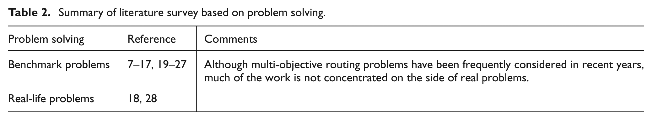
Summary of literature survey based on problem solving.

Problem solving	Reference	Comments
Benchmark problems	7–17, 19–27	Although multi-objective routing problems have been frequently considered in recent years, much of the work is not concentrated on the side of real problems.
Real-life problems	18, 28

Mathematical formulation

In VRPTW, there are N number of customers and one central department. Every customer is geologically positioned at coordinates (x, y) and has a definite demand, time window and service time. The demand from every customer must be greater than 0. The central department is indicated by the representation 0, from which all customers are supplied by distribution vehicles. In order to devise multi-objective VRPTW, the following equations are required. Equations (1) and (2) provide the formulae for management beneficial objectives, namely, the minimisation of the total distance travelled by all vehicles (D) and the total number of vehicles used (K), respectively

$$\begin{array}{c}\mathrm{Min\; D}=\sum _{\mathrm{j}=1}^{\mathrm{K}}{\mathrm{d}}_{\mathrm{j}}\hfill \\ {\mathrm{d}}_{\mathrm{j}}=\sum _{\mathrm{i}=0}^{{\mathrm{N}}_{\mathrm{j}}}{\mathrm{d}}_{(\mathrm{i},\mathrm{i}+1),\mathrm{j}}\forall \mathrm{j}=1,2,\dots ,\mathrm{K}\hfill \\ {\mathrm{d}}_{(\mathrm{i},\mathrm{i}+1),\mathrm{j}}={\mathrm{t}}_{(\mathrm{i},\mathrm{i}+1),\mathrm{j}}={[{{(\mathrm{x}}_{\mathrm{i}}-{\mathrm{x}}_{\mathrm{i}+1})}^2+{{(\mathrm{y}}_{\mathrm{i}}-{\mathrm{y}}_{\mathrm{i}+1})}^2]}^{\frac{1}{2}}\hfill \end{array}$$

(1)

$$\mathrm{Min\; K}$$

(2)

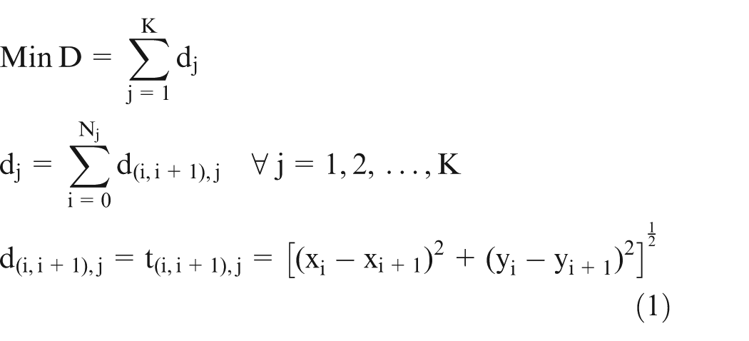
The total distance travelled by all vehicles (D) is the sum of distance travelled by all individual vehicles given by equation (1). Equation (1) shows that the distance travelled by individual vehicles (d_j) is the sum of all distances between succeeding customers from the starting point (central department) to the ending point (central department) for that vehicle. The distance and time taken for travel between the two customers (d_{(i,i + 1),j} and t_{(i,i + 1),j}) are given by Euclidean distance, as shown in equation (1). Equation (3) gives the formulae for customer beneficial objective, namely, minimisation of the total gap between ready time and issuing time

$$\begin{array}{c}\mathrm{Min\; TG}=\sum _{\mathrm{j}=1}^{\mathrm{K}}{\mathrm{CG}}_{\mathrm{j}}\hfill \\ {\mathrm{CG}}_{\mathrm{j}}=\sum _{\mathrm{i}=1}^{{\mathrm{N}}_{\mathrm{j}}}{\mathrm{g}}_{(\mathrm{i},\mathrm{j})}\forall \mathrm{j}=1,2,\dots ,\mathrm{K}\hfill \end{array}$$

(3)

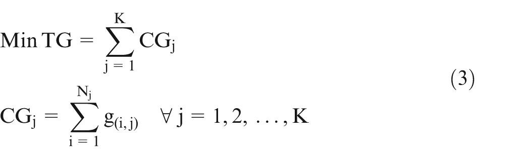
The total gap between ready time and issuing time (TG) is the sum of the combined gap time for individual vehicles shown by equation (3). The combined gap time for individual vehicles (CG_j) is the sum of all the individual customers’ gap time in that vehicle route as shown in equation (3). Equation (4) shows that the individual customer gap time (g_(i,j)) is determined by taking the difference between the arrival time and the ready time if the vehicle reaches the customer within the time windows. In this case, the vehicle waiting time is 0. Equation (4) also shows that if the vehicle reaches the customer before ready time, then the gap time is 0, but the vehicle has to spend the difference in ready time and arrival time as waiting time in order to satisfy the customer. Orders are strictly discarded if the vehicle arrives beyond the time window

$$\begin{array}{c}{\mathrm{g}}_{(\mathrm{i},\mathrm{j})}=\{\begin{array}{cc}\hfill {\mathrm{a}}_{(\mathrm{i},\mathrm{j})}-{\mathrm{e}}_{(\mathrm{i},\mathrm{j})}\hfill & \hfill \mathrm{If}{\mathrm{e}}_{(\mathrm{i},\mathrm{j})}⩽{\mathrm{a}}_{(\mathrm{i},\mathrm{j})}⩽{\mathrm{L}}_{(\mathrm{i},\mathrm{j})}\hfill \\ \multicolumn{1}{c}{0}& \hfill \mathrm{If}{\mathrm{a}}_{(\mathrm{i},\mathrm{j})}⩽{\mathrm{e}}_{(\mathrm{i},\mathrm{j})}\hfill \end{array}\hfill \\ {\mathrm{w}}_{(\mathrm{i},\mathrm{j})}=\{\begin{array}{cc}\hfill 0\hfill & \hfill \mathrm{If}{\mathrm{e}}_{(\mathrm{i},\mathrm{j})}⩽{\mathrm{a}}_{(\mathrm{i},\mathrm{j})}⩽{\mathrm{L}}_{(\mathrm{i},\mathrm{j})}\hfill \\ \multicolumn{1}{c}{{\mathrm{e}}_{(\mathrm{i},\mathrm{j})}-{\mathrm{a}}_{(\mathrm{i},\mathrm{j})}}& \hfill \mathrm{If}{\mathrm{a}}_{(\mathrm{i},\mathrm{j})}⩽{\mathrm{e}}_{(\mathrm{i},\mathrm{j})}\hfill \end{array}\hfill \end{array}$$

(4)

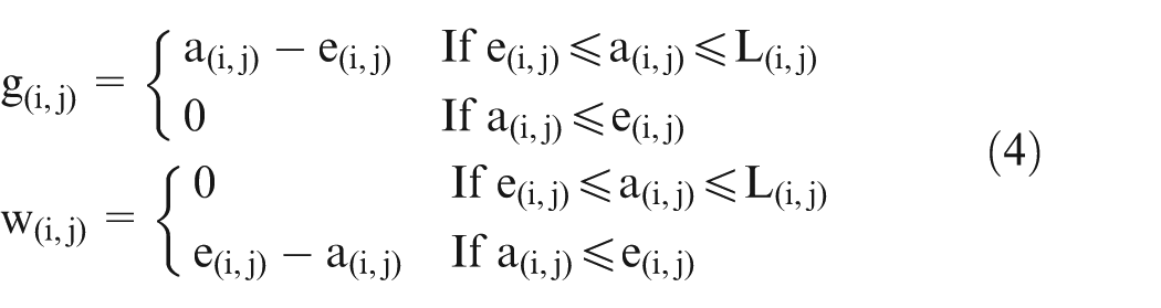
Equation (5) shows that the arrival time at each customer is the sum of arrival time of the previous customer, waiting time of the previous customer, service time of the previous customer and travel time from the previous customer to the current customer.

The demand, arrival time, waiting time and service time at the central department are 0, as denoted in equation (6). Equation (7) ensures that each vehicle should start and end at the central department

$${\mathrm{a}}_{(\mathrm{i},\mathrm{j})}={\mathrm{a}}_{(\mathrm{i}-1,\mathrm{j})}+{\mathrm{w}}_{(\mathrm{i}-1,\mathrm{j})}+{\mathrm{s}}_{(\mathrm{i}-1,\mathrm{j})}+{\mathrm{t}}_{(\mathrm{i}-1,\mathrm{i}),\mathrm{j}}$$

(5)

$${\mathrm{q}}_{(0,\mathrm{j})}={\mathrm{a}}_{(0,\mathrm{j})}={\mathrm{w}}_{(0,\mathrm{j})}={\mathrm{s}}_{(0,\mathrm{j})}=0\forall \mathrm{j}=1,2,\dots ,\mathrm{K}$$

(6)

$${\mathrm{N}}_{\mathrm{j}}+1=0\forall \mathrm{j}=1,2,\dots ,\mathrm{K}$$

(7)

The intention of this multi-objective VRPTW is to compute a set of customer-satisfied routes without refusing the following three constraints:

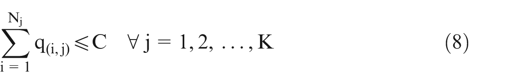
• Capacity constraint – the sum of all customer demands in a route should not go above the vehicle capacity, as given in equation (8).

• Time window constraint – each customer should be supplied within the time window, as given in equation (9).

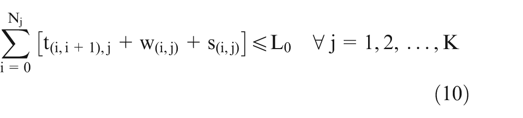
• Maximum route time constraint – each vehicle should return to the central department within the upper time bound of the central department. The maximum route time for an individual vehicle is the sum of total travel time, waiting time and service time in that route, as shown by equation (10)

$$\sum _{\mathrm{i}=1}^{{\mathrm{N}}_{\mathrm{j}}}{\mathrm{q}}_{(\mathrm{i},\mathrm{j})}⩽\mathrm{C}\forall \mathrm{j}=1,2,\dots ,\mathrm{K}$$

(8)

$${\mathrm{e}}_{(\mathrm{i},\mathrm{j})}⩽{(\mathrm{a}}_{(\mathrm{i},\mathrm{j})}+{\mathrm{w}}_{(\mathrm{i},\mathrm{j})})⩽{\mathrm{L}}_{(\mathrm{i},\mathrm{j})}\forall \mathrm{j}=1,2,\dots ,\mathrm{K}$$

(9)

$$\sum _{\mathrm{i}=0}^{{\mathrm{N}}_{\mathrm{j}}}[{\mathrm{t}}_{(\mathrm{i},\mathrm{i}+1),\mathrm{j}}+{\mathrm{w}}_{(\mathrm{i},\mathrm{j})}+{\mathrm{s}}_{(\mathrm{i},\mathrm{j})}]⩽{\mathrm{L}}_0\forall \mathrm{j}=1,2,\dots ,\mathrm{K}$$

(10)

Proposed methodology

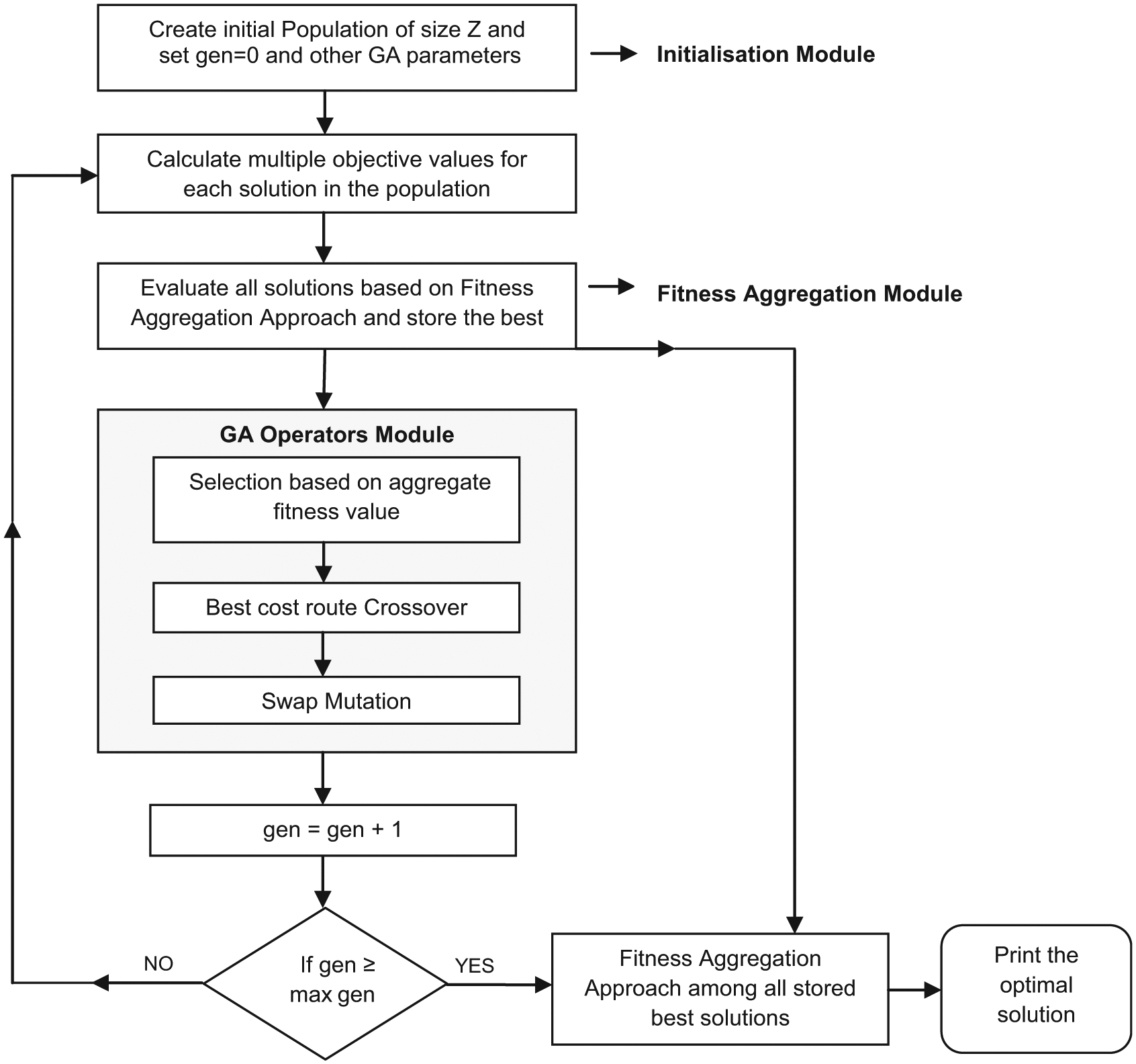
In recent years, GA has rendered itself one of the preferred methodologies for resolving multi-objective optimisation problems and VRPTW.^29,30 Many variants of the basic GA have been reported in the literature, tailored specifically to solving multi-objective problems. However, when the number of objectives raises, the convergence capability and efficiency of Pareto-based MOGA may be affected. ⁵ In this research, the fitness aggregated genetic algorithm (FAGA) is implemented through the fitness aggregation method and dedicated genetic operators to resolve the multi-objective problem. The FAGA consists of three main modules, namely, initialisation, fitness aggregation and GA operators, as shown in Figure 1. The following sections explain each module in detail.

Figure 1.

Flowchart for FAGA.

Initialisation module

In this module, an initial population is formed and GA parameters, such as population size, number of generations, crossover probability and mutation probability, are fixed. At first, the population is formed by picking a random customer to be the first customer on the first route without affecting all the constraints. In an iterative procedure, customers are then included on the first route without disturbing all the constraints. Fresh routes are formed if any one constraint is affected by a customer when positioned on any of the earlier routes. This process is replayed until all customers in a problem are fixed to routes. The complete process is replayed till Z solutions are formed in the initial population. Figure 2 shows an example for chromosome representation. In our approach, a chromosome represents a solution of length N, where N is the number of customers (in this example, N = 9).

Figure 2.

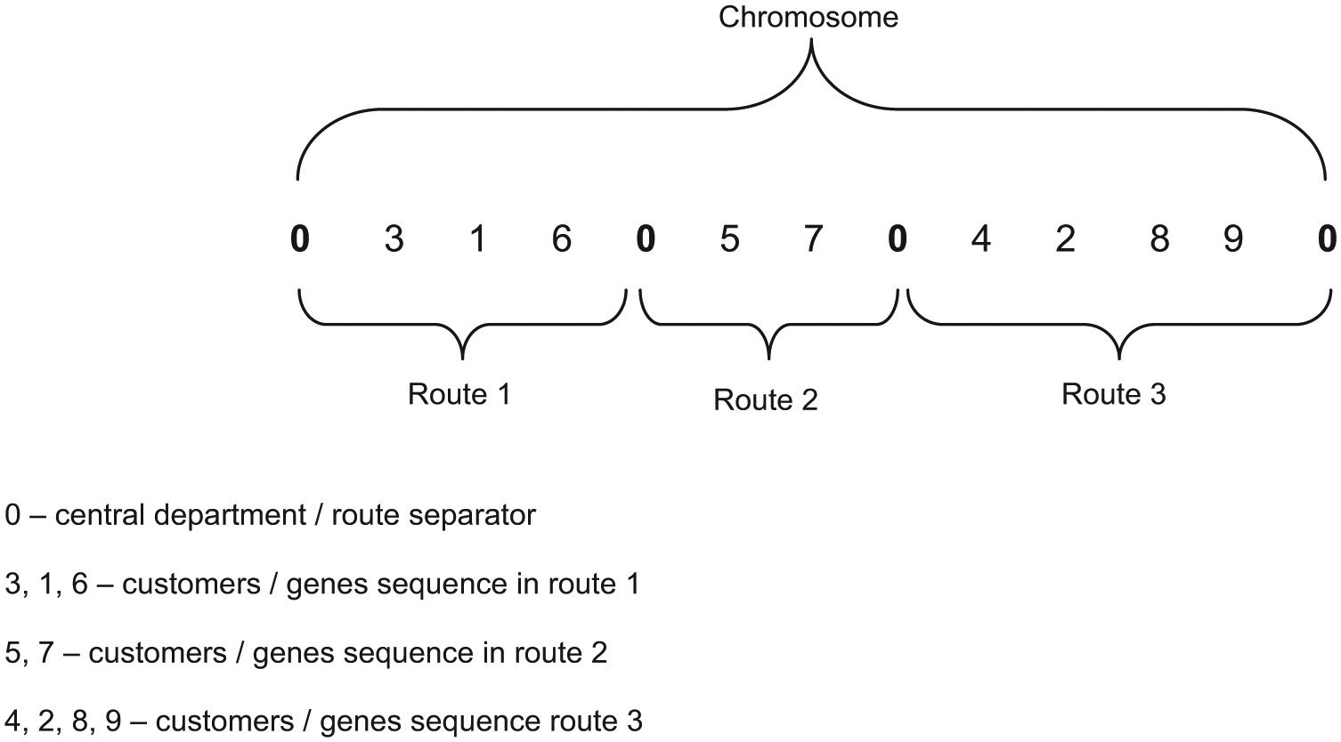
Example for chromosome representation (number of customers = 9).

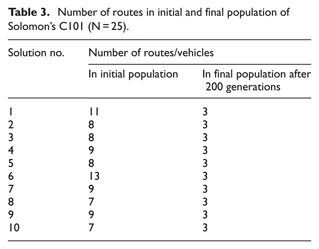
A gene in a specified chromosome shows the actual node number fixed to a customer. The order of genes in a chromosome indicates the sequence of customers within which the vehicle should travel for each route. ‘0’ represents the central department and is also used as a route separator enabling each route to start and end at the central department. The aim of the initialisation module is to create a solution pool. Each route in each solution of the pool should satisfy all the three constraints (demand constraint, time window constraint and maximum route time constraint). Hence, the objectives may be very high for all solutions in an initial pool, but after passing the crossover, mutation and the required number of generations, the objective values may attain the optimal values. Table 3 compares the number of vehicles or routes created in the initial population (population size = 10) of Solomon’s 25 customer C101 benchmark problem with the number of routes converging in the final population of the same problem after 200 generations. It may then be observed from the comparison that although the objective values are very high in the initialisation module, it converges towards optimal values after the required number of generations.

Table 3.

Number of routes in initial and final population of Solomon’s C101 (N = 25).

Solution no.	Number of routes/vehicles
	In initial population	In final population after 200 generations
1	11	3
2	8	3
3	8	3
4	9	3
5	8	3
6	13	3
7	9	3
8	7	3
9	9	3
10	7	3

Fitness aggregation module

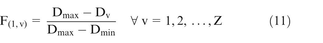
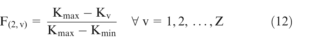
The intention of this module is to assess the fitness value for the multi-objectives, namely, the total distance travelled, the total number of vehicles used and the total gap between ready time and issuing time. The fitness value is the normalised objective value, which is used for fitness aggregation. This technique eradicates the problems linked with the choice of weight vectors for multi-objectives in the weighted sum method. Hence, it is now possible to eliminate the confusions and distractions experienced by users while getting weight vectors for multi-objectives. Initially, the fitness values for the total distance travelled by all the vehicles, the total number of vehicles used and the total gap between ready time and the issuing time for all solutions in the population are determined by equations (11)–(13). Thus, the aggregate fitness value (AFV) for every solution in the population is calculated by equation (14). Table 4 gives an example of fitness aggregation procedure and selection procedure, in which 10 solutions are considered and each solution has randomly assumed objective values (D, K and TG). The fitness values F_(1,v), F_(2,v) and F_(3,v) for the corresponding objectives are determined by equations (11)–(13) for the 10 solutions. AFV for the solutions is determined by equation (14). As it is a minimisation problem, a solution with huge AFV

$${\mathrm{F}}_{(1,\mathrm{v})}=\frac{{\mathrm{D}}_{\max }-{\mathrm{D}}_{\mathrm{v}}}{{\mathrm{D}}_{\max }-{\mathrm{D}}_{\min }}\forall \mathrm{v}=1,2,\dots ,\mathrm{Z}$$

(11)

$${\mathrm{F}}_{(2,\mathrm{v})}=\frac{{\mathrm{K}}_{\max }-{\mathrm{K}}_{\mathrm{v}}}{{\mathrm{K}}_{\max }-{\mathrm{K}}_{\min }}\forall \mathrm{v}=1,2,\dots ,\mathrm{Z}$$

(12)

$${\mathrm{F}}_{(3,\mathrm{v})}=\frac{{\mathrm{TG}}_{\max }-{\mathrm{TG}}_{\mathrm{v}}}{{\mathrm{TG}}_{\max }-{\mathrm{TG}}_{\min }}\forall \mathrm{v}=1,2,\dots ,\mathrm{Z}$$

(13)

$${\mathrm{AFV}}_{\mathrm{v}}=\frac{\sum _{\mathrm{u}=1}^{\mathrm{n}}{\mathrm{F}}_{(\mathrm{u},\mathrm{v})}}{\mathrm{n}}\{\begin{array}{c}\hfill \forall \mathrm{v}=1,2,\dots ,\mathrm{Z}\hfill \\ \multicolumn{1}{c}{\mathrm{n}=2\mathrm{for\; bi}-\mathrm{objective\; model}}\\ \multicolumn{1}{c}{\mathrm{n}=3\mathrm{for\; tri}-\mathrm{objective\; model}}\end{array}$$

(14)

is the finest solution in the population. In Table 4, solution no. 2 has the highest AFV (0.796 shown in a bold face) and it is hence, overall, the best individual in the population. Similarly, at the end of every generation the best solution is derived by the fitness aggregation approach and maintained as the best individual for the generation. Finally, at the conclusion of a necessary number of generations, a similar fitness aggregation technique is applied to all the best individuals maintained across the generations. The solution with maximum AFV among the best individuals is ultimately the best solution of the problem.

Table 4.

Example for fitness aggregation and selection based on AFV.

Solution no.	D	K	TG	F(1,v)	F(2,v)	F(3,v)	AFV	Probability	Cumulative probability	Random numbers	Selected solution for crossover
1	512	5	611	0.828	0.5	0.870	0.733	0.139	0.139	0.253	2 – best fit
2	518	4	618	0.621	1	0.768	0.796	0.151	0.290	0.466	4 – best fit
3	522	6	615	0.483	0	0.812	0.432	0.082	0.372	0.632	6
4	507	5	649	1	0.5	0.319	0.606	0.115	0.487	0.268	2 – best fit
5	531	5	602	0.172	0.5	1	0.557	0.105	0.592	0.082	1 – best fit
6	525	6	622	0.379	0	0.710	0.363	0.069	0.661	0.568	5
7	536	5	668	0	0.5	0.043	0.181	0.034	0.695	0.121	1 – best fit
8	511	4	671	0.862	1	0	0.621	0.117	0.812	0.806	8 – best fit
9	529	5	630	0.241	0.5	0.594	0.445	0.084	0.896	0.931	10
10	530	5	605	0.207	0.5	0.957	0.555	0.105	1	0.222	2 – best fit
Total							5.289	1

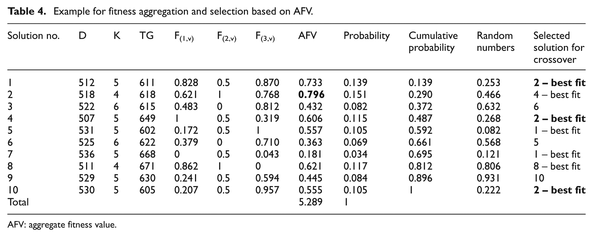
AFV: aggregate fitness value.

GA operator module

This module covers three dedicated operators, namely, a selection based on AFV, BCRC and SM. The aim of the initial operator is to select or reproduce top solutions (solutions with high AFV) for the next phase and to decrease the copy of solutions with a small AFV. Table 4 gives an example of a selection based on AFV. At first, the probability of all 10 solutions is computed by dividing particular individual AFV values with a total AFV value. Then, a cumulative probability for every solution is computed by adding a consecutive solution probability. Random numbers are formed and, depending on the range of random number in cumulative probability, the solutions are chosen for crossover. In Table 4, solution 2 has a maximum AFV (0.796) and is chosen three times, as shown in bold. Similarly, solution 1 has the second maximum AFV value (0.733) and is chosen twice. Similarly, solution 8 (AFV = 0.621) and solution 4 (AFV = 0.606) are selected one time each. Overall, out of the 10 selected solutions, 7 solutions have high AFV.

The next operator in this module is crossover. Ghoseiri and Ghannadpour ¹² confirm that normal crossover operators, such as the one-point crossover, the two-point ordered crossover and the uniform ordered crossover, may create unfeasible solutions for VRPTW. Due to the reasons outlined above, a focused genetic operator, called the BCRC, is used in this article. The major benefit of BCRC is its capacity to assist management in preserving their primary objectives (total distance and number of vehicles) in any circumstances.

The BCRC is applied with a crossover probability of P_c. Figure 3 shows the process of BCRC involving the following steps:

Figure 3.

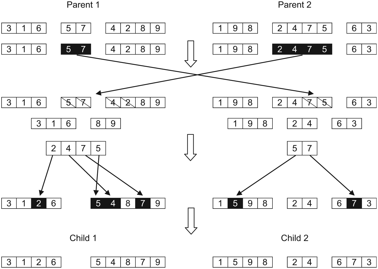
Example of the BCRC procedure.

• Step 1. Initially, the first pair of solutions is elected from the population, and they are termed as ‘parents’.

• Step 2. A random route is chosen from both the parents; for example, in Figure 3, the second route is randomly selected from the first parent and also from the second parent.

• Step 3. All the customers from the elected route of the first parent are erased from the second parent and vice versa. In this example, the customers in the elected route of the first parent (5, 7) are erased from the second parent. Similarly, the customers in the elected route of the second route (2, 4, 7 and 5) are erased from the first parent, as shown in Figure 3.

• Step 4. It restores every erased customer in the same parent at the best cost (total distance) and the best route (number of vehicles) place without affecting all the constraints. In this example, in Figure 3, the erased customers from the first parent (2, 4, 7 and 5) are reinserted in the same parent at the best cost (reduced distance) and the best route position (number of routes reduced from 3 to 2), without violating all the constraints. Similarly, the removed customers from the second parent (5, 7) are reinserted in the same parent at the best cost position (reduced distance) without violating all the constraints. As generation progresses, the number of routes converges at an optimal value. Then, the BCRC tries to reinsert the removed customers in the best cost position. After an optimal value is stabilised for both the objectives, the BCRC will reinsert the customers in the same position according to the completion of a predefined number of generations.

• Step 5. Offspring or child solutions are created which are sent to the mutation operator. The same steps are repeated for every pair of solutions in a population.

The final operator in this module is SM. SM is applied with a mutation probability of P_m. Figure 4 illustrates the SM process and it includes the following steps:

Figure 4.

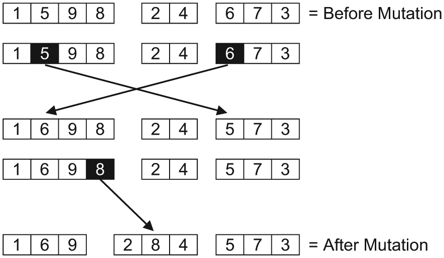
Example of the SM procedure.

• Step 1. A single solution is elected from the population.

• Step 2. One customer each from either of the two routes is randomly preferred. As an example, customer 5 is randomly selected from first route and customer 6 is randomly selected from the third route, shown in Figure 4.

• Step 3. The location of the preferred customers is exchanged if it offers the best cost position and satisfies all the constraints shown in Figure 4. Otherwise, ignore the chosen customers and go to Step 2.

• Step 4. One customer from any route of the same solution is elected randomly. The elected customer is erased from its unique position and restored with the best cost position in any of the other routes if it satisfies all the constraints. Otherwise, a similar procedure is tested with another randomly selected customer. In this example, customer 8 is selected from the first route and reinserted into the second route, shown in Figure 4.

• Step 5. The same steps are replayed for all the solutions in a population. The set of solutions generated after mutation is defined as the population for the next generation.

Computational results

Statistical examination is performed to recognise the achievement of the FAGA. The algorithm has been coded in MATLAB and run on a PC with 2.93 GHz CPU and 3 GB RAM. The experimentations employ the typical Solomon’s benchmark problem instances for VRPTW. The problems differ according to the geological locations of customers, the demands of each customer, vehicle capacity, time windows and service times. Table 5 gives the genetic operators used for experimentation. The following section provides an analysis of the genetic operators.

Table 5.

Genetic operators used for FAGA.

Parameter description	Value/type
Number of customers (N)	25
Selection type	Selection based on high AFV
Crossover type	Best cost route crossover
Crossover probability (Pc)	0.9
Mutation type	Swap mutation
Mutation probability (Pm)	0.2
Population size (Z)	50
Number of generations (max gen)	200
Number of runs (Nr)	10

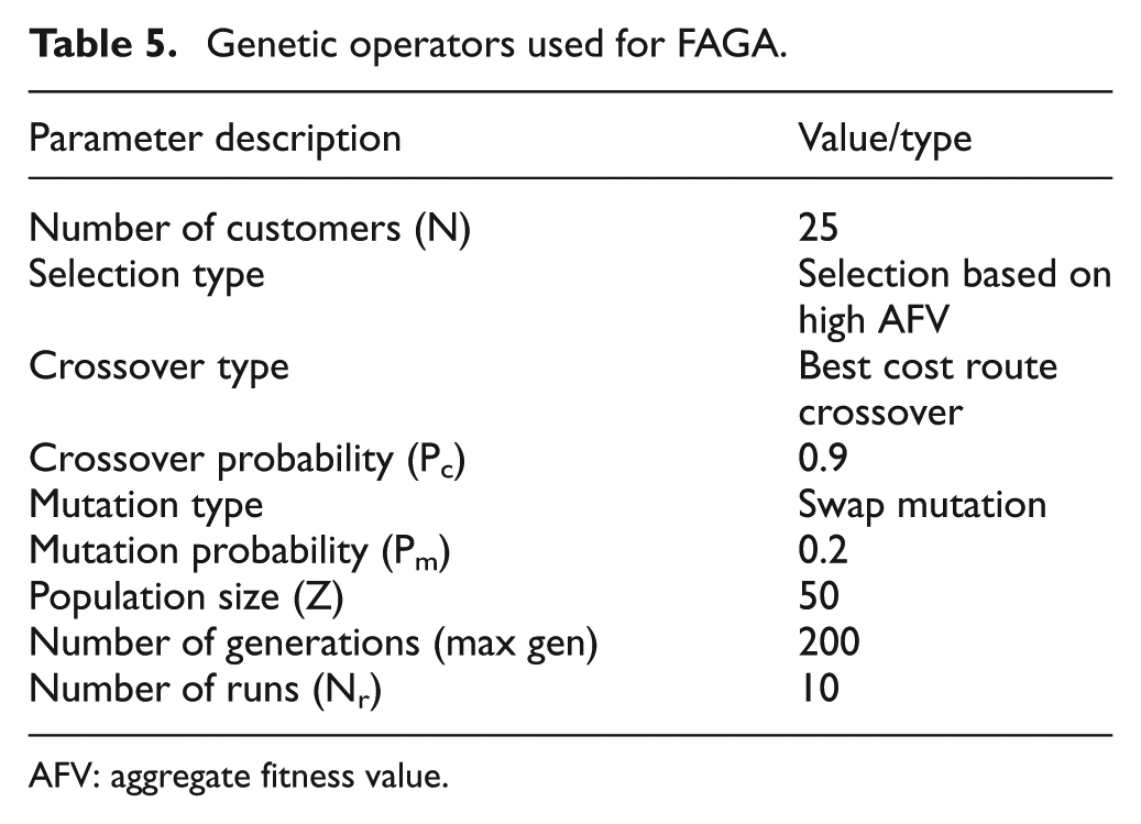
AFV: aggregate fitness value.

Genetic operators’ analysis

In our survey of the literature on the subject, the maximum values employed for BCRC probability are 0.9^14,27 and 0.8.^7,12,23 The aim of this research is to determine the set of customer-satisfied routes without significantly affecting the primary management objectives (total distance and vehicles). Hence, BCRC is employed in this article. Therefore, it is essential to search broadly for the best cost with the best route position in addition to customer satisfaction. Consequently, the maximum value of crossover probability (0.9) is employed for BCRC in this article. Similarly, in the literature, the maximum value assigned for SM is 0.2 ²⁷ and the minimum value used is 0.1. ¹⁴ In order to retain the management objectives in addition to better customer satisfaction, a deep mutation is needed for experimentation, being that even small changes in gene position can lead to major changes in all the objectives. This will enable management to satisfy customers without it having an effect on the existing resources. In order to achieve this, a high level of mutation probability (0.2) is used in this article. For population size and the number of generations, the following combinations of (Z, max gen) are tested for Solomon’s C101 benchmark instance (50, 100), (100, 100), (50, 200), (100, 200), (50, 500) and (100, 500). The optimal value for C101 (distance = 191.81 and vehicles = 3) is attained from (50, 200) to (100, 500). In order to maintain the minimum computation time, the first combination – that is, population size (50) and the number of generations (200) – is followed in this article. In many of the previous research papers, the results were validated using 10 runs. Hence, the number of runs in this research work is set to 10. The next section gives a validation for the proposed algorithm FAGA.

Results produced by FAGA for the bi-objective model

In order to validate the proposed methodology, only management objectives – that is, the total distance travelled by all vehicles and the number of vehicles – are considered as bi-objective model. In the bi-objective model, the AFV is calculated in the following way. Initially, equations (11) and (12) calculated the fitness values for the total distance travelled by all vehicles and the total number of vehicles used for all solutions in the population. The AFV for every solution in the population is then computed by equation (14). Table 6 provides an outline of the results created by FAGA for a bi-objective model in reference to a number of Solomon’s benchmark problems of VRPTW, evaluating the findings with the BK solutions. This experimentation uses 12 benchmark cases taken from different clustered sets (C sets, geographical data are clustered), randomly generated sets (R sets, geographical data are randomly created) and a combination of randomly generated and clustered sets (RC sets). Table 6 points out that out of the four C set problems, the proposed FAGA produces three problems with very similar results for both objectives in relation to BK. Moreover, out of the four RC set problems, the algorithm produces one problem with precisely similar results and three problems with approximately the same results in relation to BK. In R sets, the FAGA produces results that are very close for all the problems. Overall, out of 12 problems, the proposed algorithm produces competitive results for each problem for both objectives, as with BK. In the above evaluation, we notice that the proposed FAGA is highly competitive and effective for one of the multi-objective optimisation problems. Figure 5 shows the graphical representation of routes generated for C101 in the bi-objective model. In Figure 5, the values between the two customer nodes denote the distance between the nodes. The values within the bracket give the associated individual gap time in each of the customer nodes. The nodes without a black shading represent the customers with a high individual associated gap time, while the nodes with black shading represent the customers with a less individual associated gap time. Only five customers had less individual gap time value for the bi-objective model shown in Figure 5.

Table 6.

Results produced by FAGA for bi-objective model.

Problem no.	Best known			Results produced by FAGA (number of runs = 10)
				Best		Worst		Mean
	D	K	Ref	D	K	D	K	D	K
C101	191.81	3	14, 31	191.81	3	198.60	3	193.17	3
C105	191.81	3	31	191.81	3	193.04	3	192.18	3
C106	191.81	3	31	191.81	3	217.33	3	194.37	3
C108	191.81	3	31	194.92	3	206.35	3	200.15	3
R104	417.96	4	31	423.77	4	435.15	4	432.18	4
R106	466.48	5	31	473.56	5	489.83	5	480.67	5
R107	425.27	4	31	429.20	4	445.33	4	435.87	4
R108	398.30	4	31	407.44	4	435.62	4	422.13	4
RC102	352.74	3	31	357.57	3	359.63	3	358.09	3
RC103	333.92	3	31	333.92	3	336.14	3	334.76	3
RC105	411.30	4	15	418.53	4	426.95	4	422.63	4
RC108	294.99	3	31	299.30	3	309.75	3	305.07	3

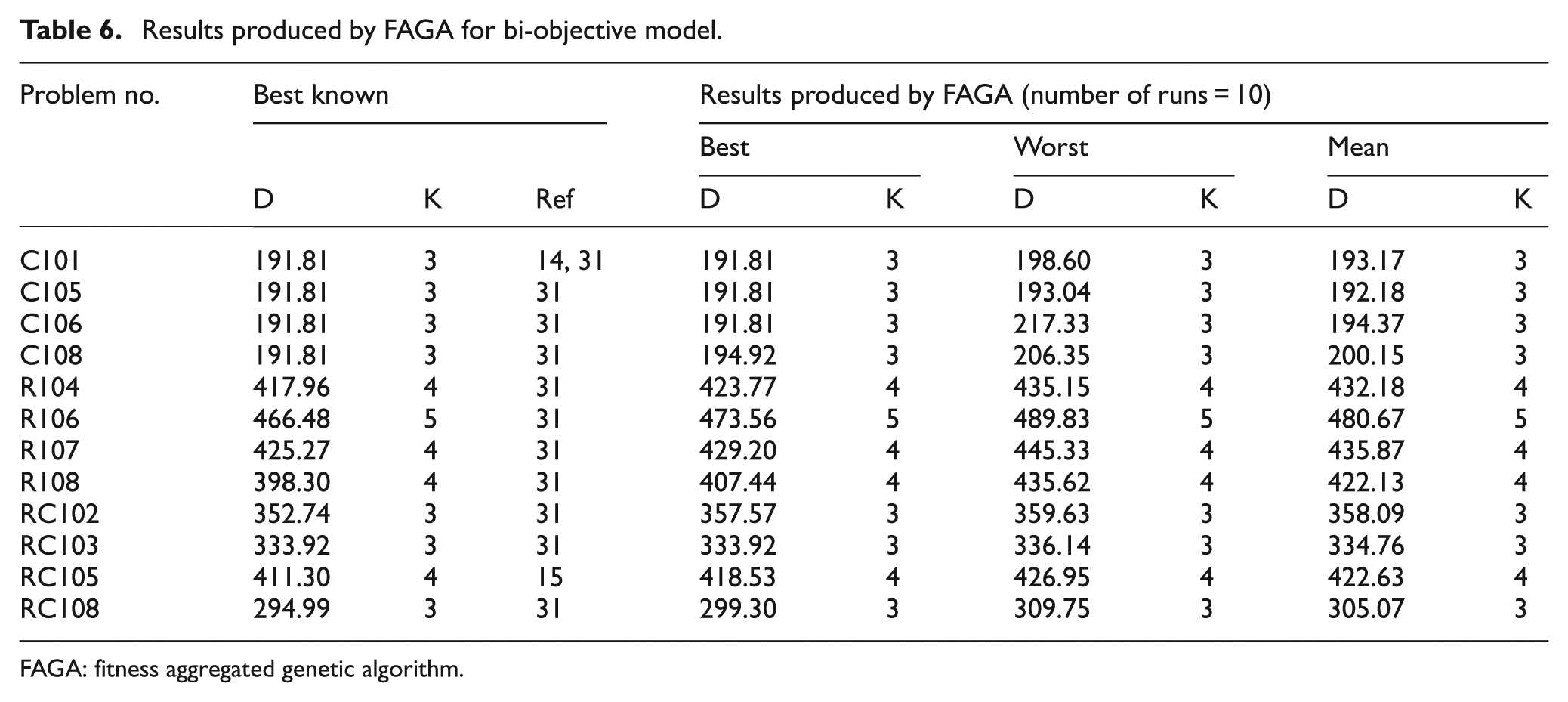
FAGA: fitness aggregated genetic algorithm.

Figure 5.

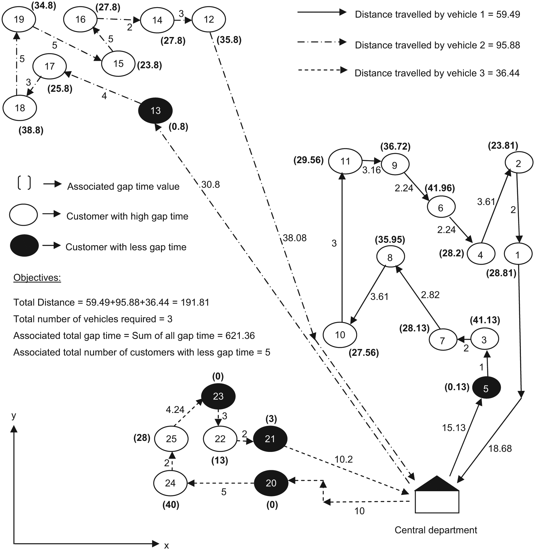
Routes created for C101 by FAGA in bi-objective model.

Results produced by FAGA for tri-objective model (with customer satisfaction)

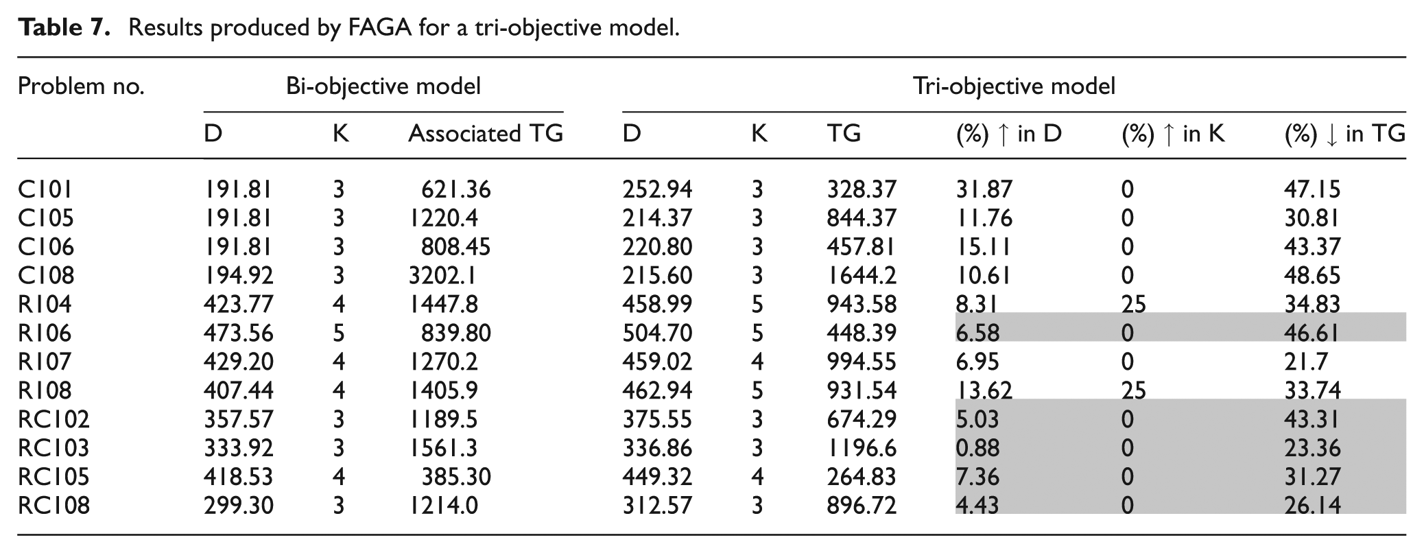
After the validation of the suggested algorithm, the third objective function, that is, the total gap between ready time and issuing time (TG), is incorporated into the bi-objective model. In Table 7, the ‘Associated TG’ value represents the corresponding value of the total gap between ready time and issuing time for the final best solution produced in the bi-objective model. The associated TG value is used to measure the percentage decrease in TG in the tri-objective model. It is used to determine how the algorithm produces customer-satisfied routes without significantly affecting the management objective values (distance and vehicle). The first analysis from Table 7 is based on the outcome of the insertion of TG on the total number of vehicles used (K). We notice in Table 7 that, out of the four C set problems, the FAGA produces all the problems of minimised TG without changing the K (total number of routes). Moreover, out of the four R set problems, the algorithm produces two problems (R106 and R107) with minimised TG, without changing K. Similarly, out of the four RC set problems, the proposed algorithm produces all the problems with minimised TG without changing K. Overall, we can observe from Table 7 that out of the 12 problems, the FAGA produces 10 problems with minimised TG without changing the second objective K. The results confirm that the insertion of the third objective (TG) does not influence the capacity of the suggested algorithm to determine the optimal number of vehicles used. The next analysis in Table 7 is based on the outcome of the insertion of the third objective (TG) on the total distance travelled (D). It is clear from the following discussion that a great percentage of reduction in TG leads to a very small rise in D. We notice from Table 7 that out of the 12 problems, 2 problems (R106 and RC102) have less than a 10% increase in D with a high reduction in TG. In R106, only a 6.58% increment in the total distance travelled leads to a 46.61% reduction in total gap time. Similarly, in RC102, only a 5.03% increment in the total distance leads to a 43.31% reduction in total gap time. In Table 7, three problems (C105, C108 and R108) have less than a 15% increase in D and a significant reduction in TG. In particular, in C108, a 10.61% increment in the total distance travelled leads to a 48.65% reduction in total gap time. In Table 7, five problems have less than a 10% increase in D and a significantly minimised TG. In particular, in RC103, a 0.88% increase in D leads to a 23.36% reduction in TG. Overall, the FAGA produces five problems with a considerably minimised TG and with very minimal increase in D without any change in K shown by a shaded representation in Table 7. Figure 6 shows the graphical representation of routes generated for C101 in the tri-objective model. In Figure 6, nodes with black shading represent the customers with a less individual gap time. In the bi-objective model, only five customers have lower gap time values, but after including the customer beneficial objectives, that is, the total gap between ready time and issuing time in the bi-objective model additional to the primary management objectives, the number of customers having a less individual gap time increases from 5 to 15, as shown in Figure 6. The above investigational study shows that the FAGA is able to determine better customer-satisfied routes by minimising the total gap time without significantly affecting the primary management objectives (distance and vehicles).

Table 7.

Results produced by FAGA for a tri-objective model.

Problem no.	Bi-objective model			Tri-objective model
	D	K	Associated TG	D	K	TG	(%) ↑ in D	(%) ↑ in K	(%) ↓ in TG
C101	191.81	3	621.36	252.94	3	328.37	31.87	0	47.15
C105	191.81	3	1220.4	214.37	3	844.37	11.76	0	30.81
C106	191.81	3	808.45	220.80	3	457.81	15.11	0	43.37
C108	194.92	3	3202.1	215.60	3	1644.2	10.61	0	48.65
R104	423.77	4	1447.8	458.99	5	943.58	8.31	25	34.83
R106	473.56	5	839.80	504.70	5	448.39	6.58	0	46.61
R107	429.20	4	1270.2	459.02	4	994.55	6.95	0	21.7
R108	407.44	4	1405.9	462.94	5	931.54	13.62	25	33.74
RC102	357.57	3	1189.5	375.55	3	674.29	5.03	0	43.31
RC103	333.92	3	1561.3	336.86	3	1196.6	0.88	0	23.36
RC105	418.53	4	385.30	449.32	4	264.83	7.36	0	31.27
RC108	299.30	3	1214.0	312.57	3	896.72	4.43	0	26.14

Figure 6.

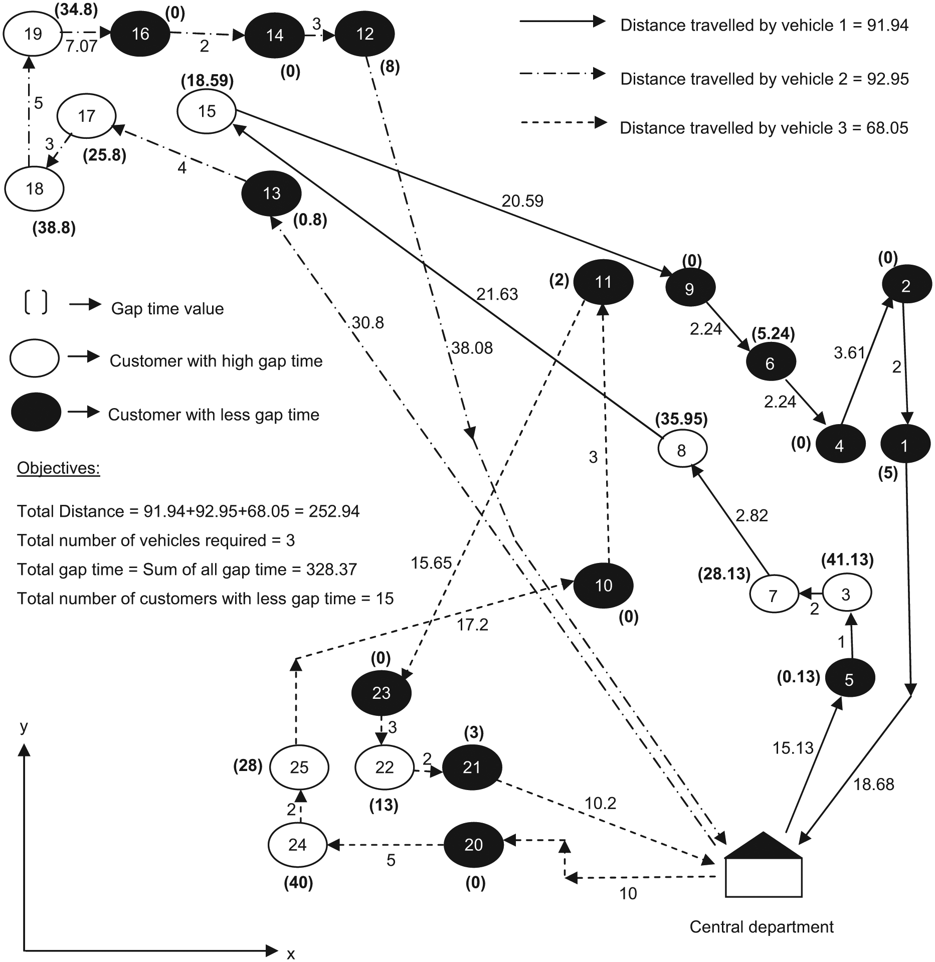
Routes created for C101 by FAGA with tri-objectives (with customer satisfaction).

Numerical illustration

Tables 8–10 provide a numerical illustration of the individual customer gap times for the tri-objective model of C101 for route 1, route 2 and route 3, respectively. Table 11 gives a numerical illustration of the individual customer gap times of the bi-objective model (distance and vehicles) for the same problem. In problem C101, the vehicle capacity is 200 and all the customers experience uniform service times of 90. Tables 8–10 give demand (q), geographical location in x- and y-coordinates (x, y), ready time and due time in time windows (e, L), distance between present and successive customers (d), service time (s), arrival time (a), waiting time (w) and individual gap time (g) for all the customers in C101 for route 1, route 2 and route 3, respectively. The individual and total distance travelled by all vehicles are determined by equation (1). Arrival time and waiting time are determined by equations (4) and (5), respectively. The individual, combined and total gap between ready time and issuing time are determined by equations (3) and (4). Before the inclusion of the third objective (TG), out of the 25 customers in C101, only 5 customers (13, 5, 20, 23 and 21) are issued goods with minimal individual gap time (0.8, 0.13, 0, 0 and 3) shown by a shaded representation in Table 11. But after the inclusion of the third objective (TG), out of the 25 customers in problem C101, 15 customers are issued goods with a very minimal individual gap time (route 1: 0, 0, 2, 0 and 3), (route 2: 0.13, 0, 5.24, 0, 0 and 5), (route 3: 0.81, 0, 0 and 8) shown by shaded representation in Tables 8–10. In particular, eight customers are issued goods at exactly their ready time (individual gap time = 0), shown by the shaded box representation in Tables 8–10. We can observe from the above analysis that in the bi-objective model, only 20% of customers are issued goods with a minimal individual gap between ready time and issuing time. However, after the inclusion of the third objective (tri-objective model), 60% of customers are issued goods with a very minimal individual gap between ready time and issuing time. Hence, the above concludes that 60% customers are highly satisfied which, in turn, motivates the afore-mentioned 60% customers to place a greater number of future orders with the same manufacturing company. It can be observed from the computational results and numerical illustrations that the proposed algorithm is able to determine customer-satisfied routes and to improve customer satisfaction by minimising the total gap between ready and issuing time. The algorithm identifies customers with a very minimal individual time gap between ready time and issuing time, and without significantly affecting the total distance travelled by all vehicles and the total number of vehicles used.

Table 8.

Individual gap times for the tri-objective model of C101 (route 1).

Customer no.	q	(x, y)	(e, L)	d	s	a	w	g
0	0	(40, 50)	(0, 1236)	15.13	0	0	0	–
5	10	(42, 65)	(15, 67)	1	90	15.13	0	0.13
3	10	(42, 66)	(65, 146)	2	90	106.13	0	41.13
7	20	(40, 66)	(170, 225)	2.82	90	198.13	0	28.13
8	20	(38, 68)	(255, 324)	21.63	90	290.96	0	35.95
15	40	(20, 80)	(384, 429)	20.59	90	402.59	0	18.59
9	10	(38, 70)	(534, 605)	2.24	90	513.18	20.82	0
6	20	(40, 69)	(621, 702)	2.24	90	626.24	0	5.24
4	10	(42, 68)	(727, 782)	3.61	90	718.48	8.52	0
2	30	(45, 70)	(825, 870)	2	90	820.61	4.39	0
1	10	(45, 68)	(912, 967)	18.68	90	917	0	5
0	0	(40, 50)	(0, 1236)	–	0	1025.68	0	–
	180			91.94				134.17

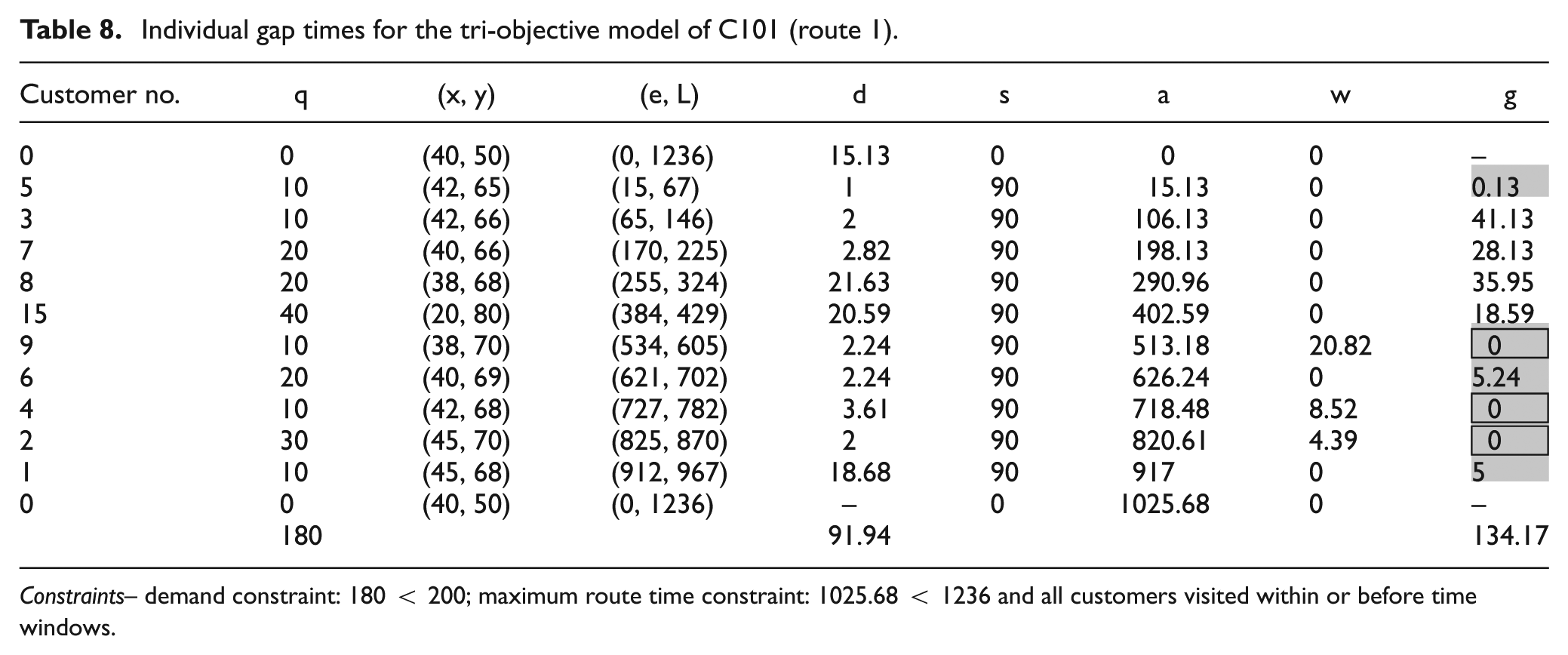
Constraints– demand constraint: 180 < 200; maximum route time constraint: 1025.68 < 1236 and all customers visited within or before time windows.

Table 9.

Individual gap times for the tri-objective model of C101 (route 2).

Customer no.	q	(x, y)	(e, L)	d	s	a	w	g
0	0	(40, 50)	(0, 1236)	30.8	0	0	0	–
13	30	(22, 75)	(30, 92)	4	90	30.8	0	0.8
17	20	(18, 75)	(99, 148)	3	90	124.8	0	25.8
18	20	(15, 75)	(179, 254)	5	90	217.8	0	38.8
19	10	(15, 80)	(278, 345)	7.07	90	312.8	0	34.8
16	40	(20, 85)	(475, 528)	2	90	409.88	65.12	0
14	10	(22, 85)	(567, 620)	3	90	567	0	0
12	20	(25, 85)	(652, 721)	38.08	90	660	0	8
0	0	(40, 50)	(0, 1236)	–	0	788.08	0	–
	150			92.95				108.2

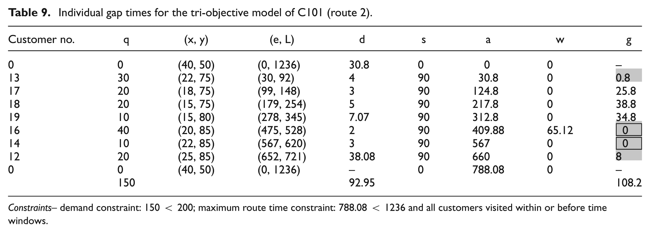
Constraints– demand constraint: 150 < 200; maximum route time constraint: 788.08 < 1236 and all customers visited within or before time windows.

Table 10.

Individual gap times for the tri-objective model of C101 (route 3).

Customer no.	q	(x, y)	(e, L)	d	s	a	w	g
0	0	(40, 50)	(0, 1236)	10	0	0	0	–
20	10	(30, 50)	(10, 73)	5	90	10	0	0
24	10	(25, 50)	(65, 144)	2	90	105	0	40
25	40	(25, 52)	(169, 224)	17.2	90	197	0	28
10	10	(35, 66)	(357, 410)	3	90	304.2	52.8	0
11	10	(35, 69)	(448, 505)	15.65	90	450	0	2
23	10	(28, 55)	(732, 777)	3	90	555.65	176.35	0
22	20	(28, 52)	(812, 883)	2	90	825	0	13
21	20	(30, 52)	(914, 965)	10.2	90	917	0	3
0	0	(40, 50)	(0, 1236)	–	0	1017.2	0	–
	130			68.05				86

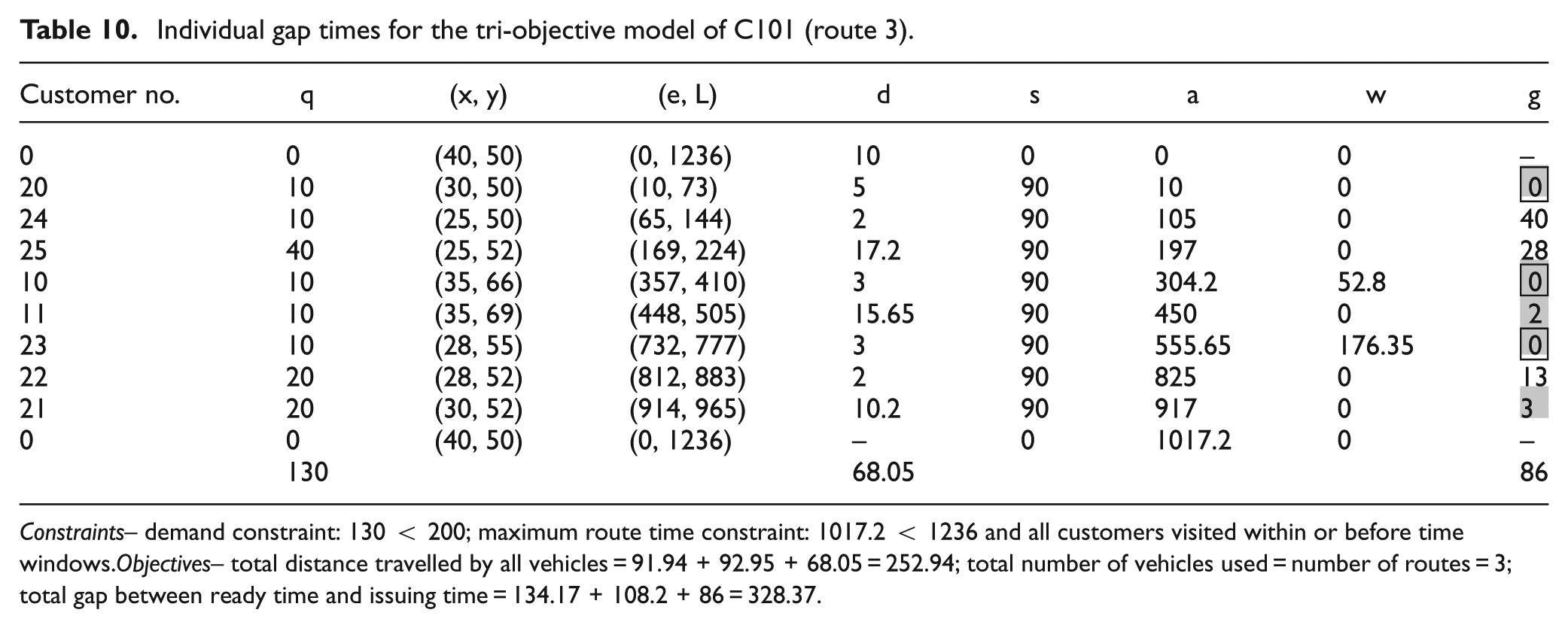
Constraints– demand constraint: 130 < 200; maximum route time constraint: 1017.2 < 1236 and all customers visited within or before time windows. Objectives– total distance travelled by all vehicles = 91.94 + 92.95 + 68.05 = 252.94; total number of vehicles used = number of routes = 3; total gap between ready time and issuing time = 134.17 + 108.2 + 86 = 328.37.

Table 11.

Individual gap times for bi-objective model of C101 (before inclusion of TG).

Customers in routes			d in routes			a in routes			g in routes
1	2	3	1	2	3	1	2	3	1	2	3
0	0	0	15.13	30.8	10	0	0	0	–	–	–
5	13	20	1	4	5	15.13	30.8	10	0.13	0.8	0
3	17	24	2	3	2	106.13	124.8	105	41.13	25.8	40
7	18	25	2.82	5	4.24	198.13	217.8	197	28.13	38.8	28
8	19	23	3.61	5	3	290.95	312.8	291.24	35.95	34.8	0
10	15	22	3	5	2	384.56	407.8	825	27.56	23.8	13
11	16	21	3.16	2	10.2	477.56	502.8	917	29.56	27.8	3
9	14	0	2.24	3	–	570.72	594.8	1017.2	36.72	27.8	–
6	12		2.24	38.08		662.96	687.8		41.96	35.8
4	0		3.61	–		755.2	815.88		28.2	–
2			2			848.81			23.81
1			18.68			940.81			28.81
0			–			1049.49			–
			59.49	95.88	36.44				321.96	215.4	84

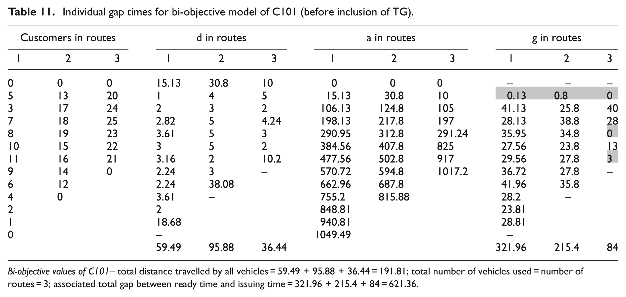
Bi-objective values of C101– total distance travelled by all vehicles = 59.49 + 95.88 + 36.44 = 191.81; total number of vehicles used = number of routes = 3; associated total gap between ready time and issuing time = 321.96 + 215.4 + 84 = 621.36.

Conclusion

In today’s competitive world, any manufacturing management cannot survive and retain customers in the long run without considering customer satisfaction. This article has considered the multi-objective VRP with time windows in distribution logistics in which the total distance travelled by all vehicles, the total number of vehicles used (management beneficial objectives) and the total gap between ready time and issuing time (customer beneficial objective) are considered. An improved GA employing the fitness aggregation method and focused operators – called the FAGA – has therefore been implemented to solve the problem. The algorithm was initially formulated as a bi-objective model with management beneficial objectives. The algorithm was validated against the best results for the bi-objective optimisation of Solomon’s benchmark problems. After validation, the third objective – that is, the total gap between ready time and issuing time – is included in the bi-objective model. The suggested algorithm achieves improved customer-satisfied routes with a minimised total gap between ready time and issuing time, and without significantly affecting the total distance travelled by all the vehicles and the total number of vehicles used. The numerical illustration shows the efficiency and significance of the suggested algorithm in improving customer satisfaction. The proposed algorithm is validated using benchmark problems with a maximum of 25 customers. However, in terms of future research, it may be extended for a greater number of customers, to real-time industry problems and to different variants of VRPs.