Effect of routing flexibility and sequencing rules on performance of stochastic flexible job shop manufacturing system with setup times: Simulation approach

Abstract

Routing flexibility is a major contributor towards flexibility of a flexible job shop manufacturing system. This article focuses on a simulation-based experimental study on the effect of routing flexibility and sequencing rules on the performance of a stochastic flexible job shop manufacturing system with sequence-dependent setup times while considering dynamic arrival of job types. Six route flexibility levels and six sequencing rules are considered for detailed study. The performance of manufacturing system is evaluated in terms of flow time related and due date–related measures. Results reveal that routing flexibility and sequencing rules have significant impact on system performance, and the performance of a system can be increased by incorporating routing flexibility. Furthermore, the system performance starts deteriorating as the level of route flexibility is increased beyond a particular limit for a specified sequencing rule. The statistical analysis of the results indicates that when flexibility exists, earliest due date rule emerges as a best sequencing rule for maximum flow time, mean tardiness and maximum tardiness performance measures. Furthermore, smallest setup time rule is better than other sequencing rules for mean flow time and number of tardy jobs performance measures. Route flexibility level two provides best performance for all considered measures.

Introduction

With the globalization of manufacturing, manufacturers face an increasingly uncertain external environment such as the rate of change in customer expectations, global competition and technology advancement.^1,2 There is an increasing trend towards higher productivity, higher product variety and shorter lead time. In this environment, manufacturing industries are forced to execute a system that can provide efficiency and flexibility. ³ Therefore, the emergence of flexible job shop manufacturing system is an important development in this direction.

Gupta and Buzacott ⁴ defined flexibility as ‘the ability of the manufacturing system to cope with the changes effectively’. Chan ⁵ described flexibility of a manufacturing system as ‘the ability to cope with changes in product mix, volume or timing of its activity in an efficient and effective manner’. Flexibility is an important attribute of manufacturing systems which enables companies to become competitive in a very dynamic environment. The flexibility of a system is dependent upon its components (machines, material handling systems, etc.), capabilities, interconnections, and the mode of operation and control. ³

Buzacott ⁶ classified flexibility into two main groups as job flexibility and machine flexibility. Browne et al. ⁷ described eight types of flexibilities, namely, machine flexibility, process flexibility, product flexibility, routing flexibility, volume flexibility, expansion flexibility, operation flexibility, and production flexibility. Sethi and Sethi ⁸ added three more types of flexibilities such as material handling flexibility, programme flexibility and market flexibility to the classification of Browne et al. ⁷ Chen et al. ⁹ addressed flexibility and classified it into three main classes as follows: product flexibility, marketing flexibility and infrastructural flexibility. Similar to Chen et al., ⁹ Benjaafar and Ramakrishnan ¹⁰ classified flexibility into two main categories, namely, product-related flexibility and process-related flexibility. Vokurka and Leary-Kelly ¹¹ also analysed flexibility using a more general perspective and described four additional flexibility dimensions as follows: automation flexibility, labour flexibility, new design flexibility and delivery flexibility. Jain et al. ¹² provided a review on manufacturing flexibility.

Routing flexibility is one of the major contributors towards flexibility of a flexible job shop manufacturing system. It is the ability of the manufacturing system to produce jobs economically and efficiently by alternative routes through the system. Mohamed et al. ¹³ measure routing flexibility by a number of existing actual production routes that can be used by a job resulting from machine loading. Routing flexibility provides better schedule as it efficiently balances machine loads, minimizes system utilization and work-in-process inventory, improves the productivity of machine shop and continuously produces the jobs despite the occurrence of unanticipated events such as machine failure, downtimes, rush orders, late receipt of machine tools and pre-emptive schedule. ¹⁴ However, its implementation incurs a huge cost for the installation of flexible machines, automated tool changers and fixtures and even machine operators possessing multiple skills. Therefore, the system designers or manufacturing managers must determine the appropriate level of route flexibility for a specific system configuration in order to balance benefits and costs incurred.^14–16

Flexible job shop scheduling problem is an extension of classical job shop scheduling problem. It consists of two sub-problems: assignment of an operation to an appropriate machine and sequencing the operations on each machine. Flexible job shop scheduling problem, a more complex version of the job shop scheduling problem, is strongly non-deterministic polynomial-time (NP)-hard. ¹⁷ In a stochastic flexible job shop (SFJS) manufacturing system, at least one parameter of the job (release time, processing times/setup times) is probabilistic. ¹⁸ Setup time is a time which is required to prepare the necessary resources such as machines to perform a task. ¹⁹ In many real-life situations, a setup operation often occurs while shifting from one operation to another. Sequence-dependent setup time depends on both current and immediately preceding operation. ¹⁹ Scheduling problems with sequence-dependent setup times are among the most difficult classes of scheduling problems. ²⁰ It has been pointed out by some authors that limited research on job shop scheduling problems with sequence-dependent setup times is available.^21,22

Due to complexity of flexible job shop scheduling problems with sequence-dependent setup times, the research in this field is rather limited. Instead, the researchers focused more on flexible job shop scheduling problems. Bruker and Schlie ²³ were first among the researchers to address the flexible job shop scheduling problem. They proposed a polynomial algorithm to solve the assignment and scheduling problems with two jobs. Chan et al. ²⁴ proposed an adaptive genetic algorithm for distributed scheduling problems in multi-factory and multi-product environment. They introduced a new crossover mechanism named dominated gene crossover to enhance the performance of genetic search and eliminating the problem of determining the optimal crossover rate. Chan et al. ²⁵ proposed an innovative genetic algorithm–based approach for solving resource constraints’ flexible job shop scheduling problems. Chan et al. ²⁶ proposed a genetic algorithm with dominant gene approach to deal with distributed flexible manufacturing system scheduling problems subjected to alternative production routing and machine maintenance constraint. The optimization performance of the proposed approach is compared with the simple genetic algorithm to demonstrate its reliability. Moon et al. ²⁷ developed mixed-integer linear programming formulations and proposed a genetic algorithm approach for scheduling job shop problems with alternative routings. Chan et al. ²⁸ combined lot streaming and assembly job shop scheduling problem, extending lot streaming applicability to both machining and assembly. They proposed an efficient algorithm using genetic algorithms and simple dispatching rules for the problem. Chan et al. ²⁹ extended previous work of Chan et al. ²⁸ on lot streaming to assembly job shop scheduling problem by allowing part sharing among distinct products. They proposed an evolutionary approach with genetic algorithm in addition to the use of simple dispatching rules. The computational results suggest that the proposed algorithm outperforms the previous one (Chan et al. ²⁸ ). Chan et al. ³⁰ proposed a new approach using genetic algorithm to determine the lot streaming conditions and to solve job shop scheduling problems simultaneously. Wong et al. ³¹ addressed a resource-constrained assembly job shop scheduling problem with lot streaming technique. To enhance the model usefulness, two experimental factors as common part ratio and workload index are introduced. They proposed an innovative genetic algorithm approach and showed by computational experiments that the proposed approach outperforms the particle swarm optimization. Souier et al. ³² studied a flexible manufacturing system with routing flexibility. They showed how the different metaheuristics are adapted for solving the alternative routing selection problem in real time in order to reduce the congestion in the system by selecting a routing for each part among its alternative routings. They highlighted the impact of the real-time rescheduling of parts contained in the loading station on system performances when these metaheuristics are applied. The system performance measured in terms of production rate, machines and material handling utilization rate shows that for an overloaded system, the real-time rescheduling outperforms the case without rescheduling. Dousthaghi et al. ³³ presented a new mixed-integer non-linear programming model for the economic lot and delivery scheduling problem in a flexible job shop with sequence-independent setup times and unrelated parallel machines on which the planning horizon length is finite and each product has a shelf life without any spoilage. An efficient hybrid particle swarm optimization is proposed to solve large-sized problems. It is found that the proposed algorithm provides better solutions over lower bounds and common cycle approach solutions. Nejad and Fattahi ³⁴ studied a flexible job shop scheduling problem with sequence-independent setup times and cyclic jobs. The objective of the problem is to minimize the total cost including delay costs, setup costs and holding costs. To find the schedule in the short-term horizon, a mathematical model (mixed-integer linear programming) for small size problems and a genetic algorithm for medium and large size problems are proposed. Results show that the proposed genetic algorithm provides a better performance than the simulated annealing algorithm.

From the viewpoint of literature review in the area of flexible job shop scheduling with consideration of sequence-dependent setup times and routing flexibility, Yu and Ram ³⁵ proposed a response threshold model based on bio-inspired scheduling approach for scheduling dynamic job shop problems with sequence-dependent setups and routing flexibility. The proposed model outperforms the auction-based model and dispatching rule–based approach. Rossi and Dini ³⁶ presented a disjunctive graph representational model of flexible job shop scheduling problems with routing flexibility, sequence-dependent setups and transportation times to minimize makespan. They presented an ant colony system and compared with alternative approaches to prove its effectiveness. Fantahun and Mingyuan ²² proposed a lot streaming technique for job shop scheduling problems with routing flexibility, sequence-dependent setup times, machine release dates and lag time to minimize makespan. They proposed parallel genetic algorithm and showed by computational analysis that it performs better than a sequential algorithm. Fantahun and Mingyuan ³⁷ presented a mathematical model for job shop scheduling problems by incorporating alternative routings, sequence-dependent setup times, attached or detached setup times, machine release dates and time lag requirements. They proposed a parallel genetic algorithm for the problem. The computational results indicate that the proposed algorithm provides better performance than the simple genetic algorithm.

From the viewpoint of literature review in the area of studying the impact of routing flexibility in a manufacturing system, Chan ⁵ studied the effect of dispatching and routing decisions on the performance of a flexible manufacturing system. They considered three routing policies, that is, no alternative routings, dynamic alternative routing and planned alternative routing with infinite and finite capacity buffer between machines. The performance measures considered are makespan, average machine utilization, average flow time and average delay at input buffers. Results indicate that for infinite capacity buffer between machines, alternative routing planned policy combined with shortest processing time (SPT) dispatching rule provides the best performance for all considered measures. For finite capacity buffer between machines, dynamic alternative routing policy provides the best performance for all considered measures except for average delay at local input buffer. Chan ¹⁵ presented a framework based on a Taguchi experimental design for studying the effect of different levels of route flexibility on flexible manufacturing system performance. The author concluded that increasing routing flexibility cannot be treated as a key role in the system improvement, and route flexibility level (RFL) two provides best system performance. Chan et al. ³⁸ studied the effect of routing flexibility on a flexible manufacturing system performance by considering physical and operating characteristics of alternative machines. The performance of flexible manufacturing system is measured in terms of makespan. They concluded that flexibility can be increased strategically up to a certain level with benefits while considering the physical and operating characteristics of the system. Caprihan and Wadhwa ³⁹ presented a framework based on Taguchi experimental design to study the impact of routing flexibility on a flexible manufacturing system performance. The performance of flexible manufacturing system is measured in terms of makespan. They concluded that increase in routing flexibility, at the cost of an associated penalty on operation processing time, is not beneficial. There is an optimum level of routing flexibility beyond which the performance of system starts decreasing. Joseph and Sridharan ³ evaluated routing flexibility of a flexible manufacturing system in terms of measures such as routing efficiency, routing versatility and routing variety with dynamic arrival of part types for processing in the system. Two cases with respect to processing times of operations on alternative machines are considered. Results indicate that the routing flexibility level and case (with/without penalty for processing times on alternative machines) have significant effect on system performance. Joseph and Sridharan ⁴⁰ focused on a simulation-based experimental study of the effects of routing flexibility, sequencing flexibility and sequencing rules (SRLs) on the performance of a flexible manufacturing system. The performance of the system is measured in terms of measures related to flow time and tardiness of parts. They concluded that system performance improves by incorporating routing flexibility, sequencing flexibility or both. The benefits of these flexibilities diminish at higher flexibility levels. The SRLs, that is, earliest due date (EDD) and earliest operation due date, provide better performance for all considered measures. Joseph and Sridharan^40,41 extended the previous work by developing multiple regression–based metamodels using simulation results.

A SRL selects the next job to be processed from the set of jobs awaiting processing. SRLs are also termed as scheduling rules or dispatching rules. Sequencing of jobs in a manufacturing system is a combinatorial problem. ⁴² Haupt ⁴³ classified SRLs as process time–based rules, due date–based rules, combination rules and rules that are neither process time based nor due date based. Panwalkar and Iskander ⁴⁴ provided a review of SRLs used in manufacturing systems. Blackstone et al. ⁴² presented a state-of-the-art survey of SRLs used in the job shop manufacturing system. Chan et al. ⁴⁵ analysed the dynamic dispatching rules for a flexible manufacturing system. To the best of the author’s knowledge, Wilbrecht and Prescott ⁴⁶ were first among researchers to study the influence of setup times on job shop manufacturing system performance. They proposed a setup-oriented SRL, that is, select a job with shortest setup time for the imminent operation (SIMSET) and conducted computational experiments. Results indicated that the SIMSET rule outperforms the existing SRLs, that is, random, EDD, shortest process time, longest process time, shortest run time and longest run time. Kim and Bobrowski ¹⁸ reported that the performance of SIMSET rule is the best for mean flow time measure when a job shop scheduling problem with sequence-dependent setup times is considered. Barman ⁴⁷ reported that the SPT rule is a benchmark rule for minimization of mean flow time and number of tardy jobs, while EDD rule is a benchmark rule for minimizing the maximum tardiness performance measure. The mean tardiness performance of various rules is a function of job and shop characteristics and cannot be optimized by any particular rule. Chan et al. ⁴⁵ and Sabuncuoglu and Hommertzheim ⁴⁸ reported that SPT SRL performs well for mean flow time performance measure in a flexible manufacturing system. Lee and Kim ⁴⁹ reported that the smallest ratio of processing time to number of remaining operations (POPN), smallest ratio of processing time to remaining work (PWRK), maximum operations remaining (MOPN) and most work remaining (MWRK) rules provide better performance as compared to other SRLs for makespan measure. In a flexible manufacturing system, where alternative process plans are available, SPT and first-come first-served (FCFS) rules provide better performance than the EDD SRL for mean flow time and mean tardiness measures. ⁵⁰ Recently, Vinod and Sridharan ⁵¹ proposed five setup-oriented SRLs, that is, (1) select a job with shortest sum of setup time and processing time, (2) select a job with similar setup and SPT, (3) select a job with similar setup and EDD, (4) select a job with similar setup and earliest modified due date (EMDD) and (5) select a job with similar setup and shortest sum of setup time and processing time for dynamic job shop scheduling problems with sequence-dependent setup times. The proposed rules provide better performance compared with already existing SRLs, that is, first-in first-out (FIFO), SPT, EDD, EMDD, critical ratio (CR), SIMSET and job with similar setup and critical ratio (JCR) for mean flow time, mean tardiness, mean setup time and mean number of setup performance measures. They also observed that in some cases even the already existing SRLs such as SPT and SIMSET perform well, while the performance of other rules was the worst.

The reviewed literature reveals that in past no attempt has been made to assess the effect of routing flexibility on the performance of SFJS manufacturing system with setup time consideration. Furthermore, the effect of SRLs and RFLs for the said manufacturing system with sequence-dependent setup times has also not been addressed. This motivates the authors to investigate the problem, and this is the first study in this area. To describe the operations, a discrete-event simulation model of the SFJS manufacturing system under different levels of route flexibility is developed. Six RFLs along with six SRLs are considered for detailed investigation. Job types are processed on alternative machines depending upon the level of route flexibility. The performance of the system is evaluated in terms of flow time–related measures, that is, mean flow time and maximum flow time and due date–related measures, that is, mean tardiness, maximum tardiness and number of tardy jobs. The simulation results of the study are subjected to statistical analysis. Analysing the performance of SFJS with sequence-dependent setup times under different RFL and SRL policies is the significant contribution of the research work presented in this article.

The remainder of the article is organized as follows. The next section ‘Job shop configuration’ describes salient aspects of the configuration of the SFJS scheduling problem. The outline for the development of simulation model is explained in section ‘Structure of simulation model’. Section ‘Experimental design for simulation study’ presents the details of simulation experimentations. Section ‘Simulation results and analyses’ provides the analysis of experimental results. Finally, section ‘Conclusion’ gives concluding remarks and directions for future work.

Job shop configuration

In this study, a job shop manufacturing system with 10 machines is selected. The machines are not identical and capable of performing different operations. However, change in setup is required to accommodate different job types. The shop floor consisting of one load/unload station and 10 different machines with local input buffers and output buffers is shown in Figure 1. This configuration is determined based on the configuration of job shop considered by various researchers.^51–53 It is pointed out by researchers that six machines are sufficient to represent the complex structure of a job shop manufacturing system,^46,54 and job shop size variations do not significantly affect the relative performance of SRLs.^{42,46,52,54,55} For the same reason, most of the researchers addressed a job shop scheduling problem with less than 10 machines^35,36,56 as it is cheaper to simulate a small size shop. ⁴²

Figure 1.

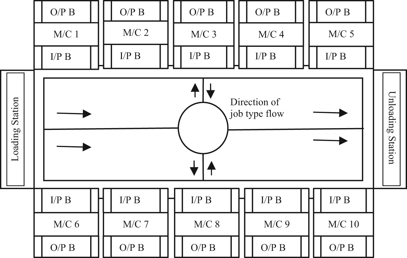
Layout of the flexible job shop manufacturing system.

Job data

Six different types of jobs, that is, job type A, job type B, job type C, job type D, job type E and job type F, arrive at the manufacturing system. All the job types have equal probability of arrival. Job type A has five operations, job type B has four operations, job type C has four operations, job type D has five operations, job type E has four operations and job type F has five operations. In this study, routing flexibility is an experimental factor. Thus, the RFLs 0–5 are considered for experimental investigation. Each operation of the job may be performed on a set of alternative machines. At RFL0, the route of the job is fixed, so no alternative machines are possible and hence routing rule is not required. RFL1, RFL2, RFL3, RFL4 and RFL5 are represented with one, two, three, four and five alternative machines, respectively.

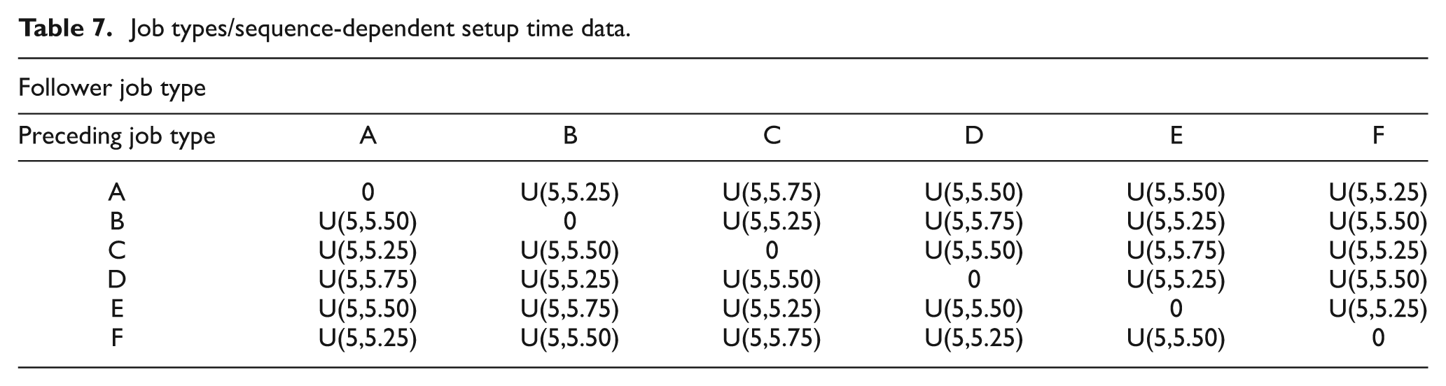
Processing times and setup times of each job are stochastic and assumed to be uniformly distributed on each machine. Processing time changes according to the job type and route of the job. This is an example case study. Since routing flexibility is an experimental factor, the processing times on alternative machines at different RFLs are shown in Tables 1–6. Sequence-dependent setup time encountered while shifting from one job type to another is given in Table 7.

Table 1.

Job types/processing time data (RFL0).

Job type	Operation	Alternative machines
		1	2	3	4	5	6	7	8	9	10
A	1	U(10,11)	x	x	x	x	x	x	x	x	x
	2	x	x	x	x	x	U(14,15)	x	x	x	x
	3	x	x	x	x	x	x	x	x	x	U(17,18)
	4	x	U(16,17)	x	x	x	x	x	x	x	x
	5	x	x	x	U(18,19)	x	x	x	x	x	x
B	1	x	x	x	x	x	x	x	U(17,18)	x	x
	2	x	x	U(10,11)	x	x	x	x	x	x	x
	3	x	x	x	x	U(19,20)	x	x	x	x	x
	4	x	x	x	x	x	x	x	x	x	U(13,14)
C	1	x	x	x	x	x	x	U(17,18)	x	x	x
	2	x	x	x	x	x	x	x	x	U(11,12)	x
	3	x	x	U(16,17)	x	x	x	x	x	x	x
	4	U(13,14)	x	x	x	x	x	x	x	x	x
D	1	x	x	x	x	U(12,13)	x	x	x	x	x
	2	x	x	x	x	x	x	U(19,20)	x	x	x
	3	x	x	x	x	x	x	x	x	U(16,17)	x
	4	x	U(10,11)	x	x	x	x	x	x	x	x
	5	x	x	x	U(17,18)	x	x	x	x	x	x
E	1	x	U(13,14)	x	x	x	x	x	x	x	x
	2	x	x	x	x	x	x	x	U(19,20)	x	x
	3	U(10,11)	x	x	x	x	x	x	x	x	x
	4	x	x	x	x	x	x	x	x	x	U(16,17)
F	1	x	x	x	x	x	U(19,20)	x	x	x	x
	2	x	x	x	x	x	x	x	x	U(13,14)	x
	3	U(15,16)	x	x	x	x	x	x	x	x	x
	4	x	x	U(10,11)	x	x	x	x	x	x	x
	5	x	x	x	x	U(14,15)	x	x	x	x	x

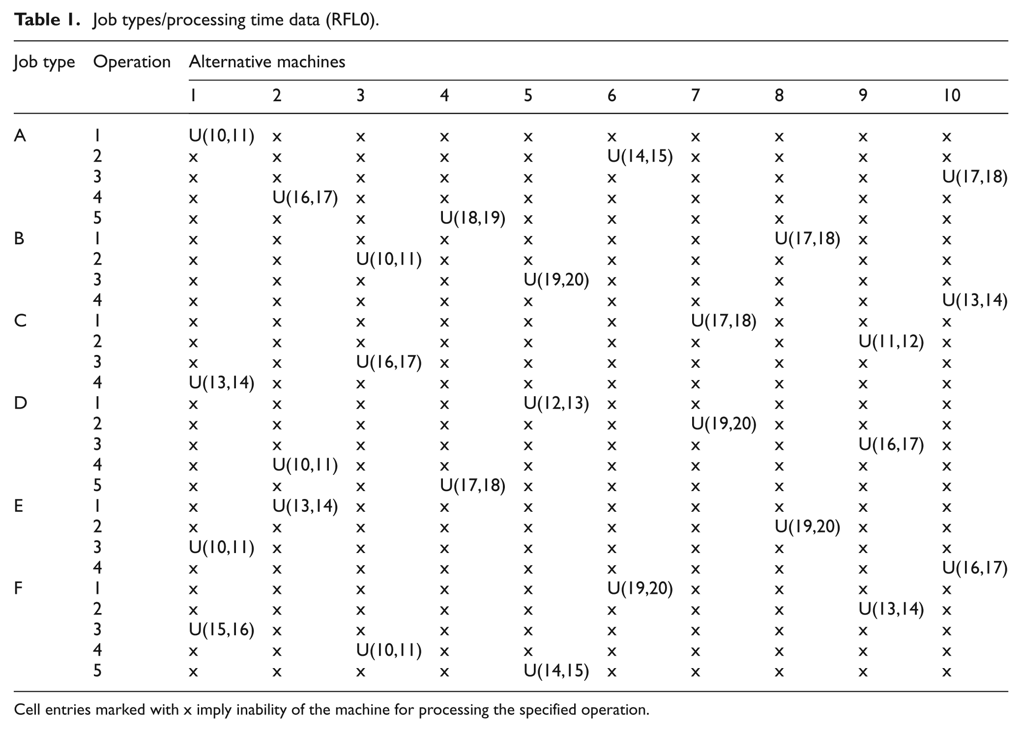
Cell entries marked with x imply inability of the machine for processing the specified operation.

Table 2.

Job types/processing time data (RFL1).

Job type	Operation	Alternative machines
		1	2	3	4	5	6	7	8	9	10
A	1	U(10,11)	x	x	x	x	x	x	U(11,12)	x	x
	2	x	x	U(12,13)	x	x	U(14,15)	x	x	x	x
	3	x	x	x	x	U(18,19)	x	x	x	x	U(17,18)
	4	x	U(16,17)	x	x	x	x	U(15,16)	x	x	x
	5	x	x	x	U(18,19)	x	x	x	x	U(19,20)	x
B	1	U(16,17)	x	x	x	x	x	x	U(17,18)	x	x
	2	x	x	U(10,11)	x	x	U(11,12)	x	x	x	x
	3	U(18,19)	x	x	x	U(19,20)	x	x	x	x	x
	4	x	x	x	U(12,13)	x	x	x	x	x	U(13,14)
C	1	x	U(18,19)	x	x	x	x	U(17,18)	x	x	x
	2	x	x	x	U(10,11)	x	x	x	x	U(11,12)	x
	3	x	x	U(16,17)	x	x	U(15,16)	x	x	x	x
	4	U(13,14)	x	x	x	x	x	x	U(14,15)	x	x
D	1	x	x	x	x	U(12,13)	x	x	x	x	U(13,14)
	2	U(18,19)	x	x	x	x	x	U(19,20)	x	x	x
	3	x	x	U(15,16)	x	x	x	x	x	U(16,17)	x
	4	x	U(10,11)	x	x	x	U(11,12)	x	x	x	x
	5	x	x	x	U(17,18)	x	x	x	U(18,19)	x	x
E	1	x	U(13,14)	x	x	x	x	x	x	U(14,15)	x
	2	x	x	x	x	U(18,19)	x	x	U(19,20)	x	x
	3	U(10,11)	x	x	x	x	x	U(11,12)	x	x	x
	4	x	x	U(15,16)	x	x	x	x	x	x	U(16,17)
F	1	x	x	x	U(18,19)	x	U(19,20)	x	x	x	x
	2	x	U(12,13)	x	x	x	x	x	x	U(13,14)	x
	3	U(15,16)	x	x	x	x	x	x	x	x	U(16,17)
	4	x	x	U(10,11)	x	x	x	U(11,12)	x	x	x
	5	x	x	x	x	U(14,15)	x	x	U(15,16)	x	x

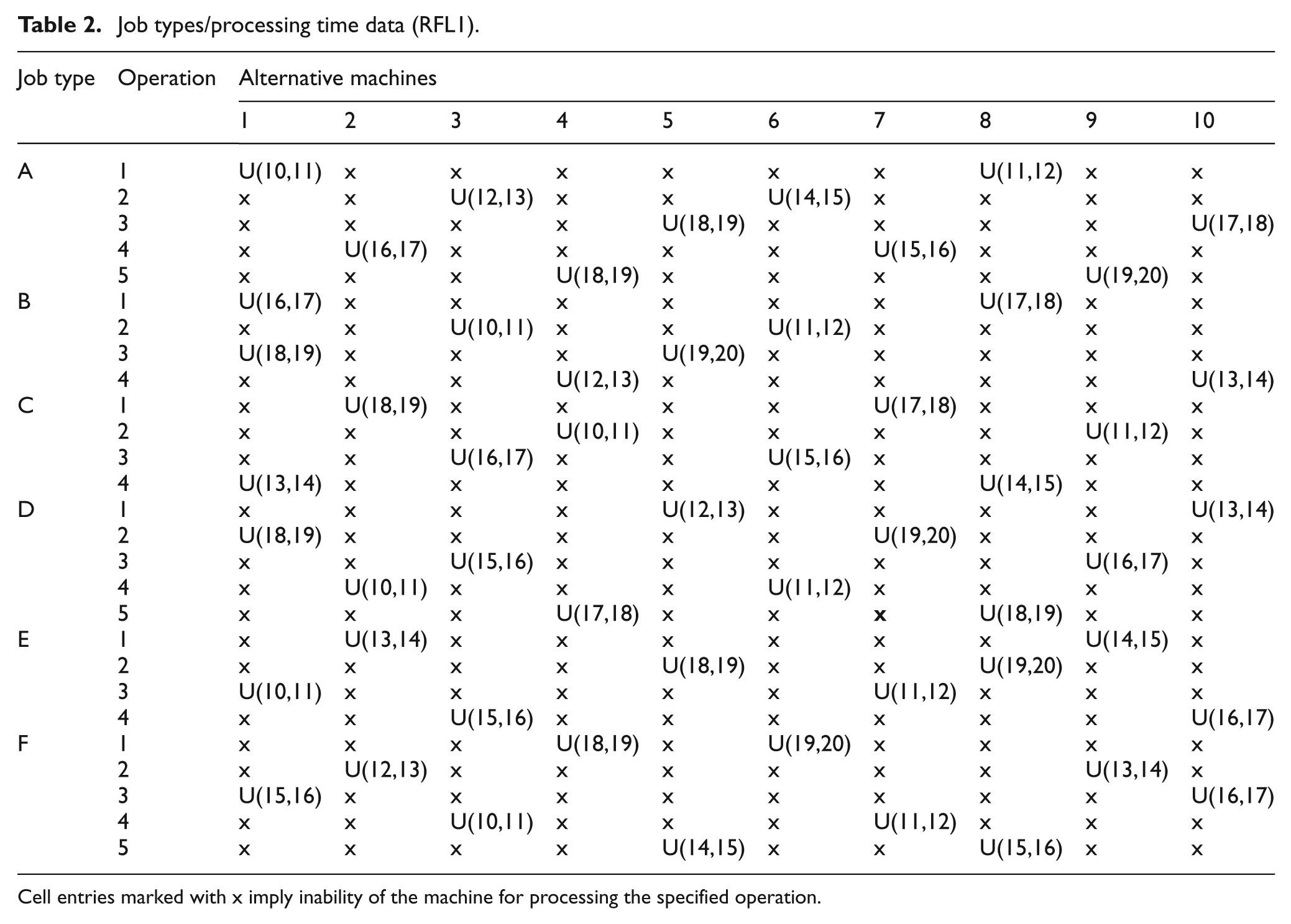
Cell entries marked with x imply inability of the machine for processing the specified operation.

Table 3.

Job types/processing time data (RFL2).

Job type	Operation	Alternative machines
		1	2	3	4	5	6	7	8	9	10
A	1	U(10,11)	x	x	U(12,13)	x	x	x	U(11,12)	x	x
	2	x	x	U(12,13)	x	x	U(14,15)	x	x	U(13,14)	x
	3	x	U(16,17)	x	x	U(18,19)	x	x	x	x	U(17,18)
	4	x	U(16,17)	x	x	x	x	U(15,16)	U(14,15)	x	x
	5	U(17,18)	x	x	U(18,19)	x	x	x	x	U(19,20)	x
B	1	U(16,17)	x	x	x	U(15,16)	x	x	U(17,18)	x	x
	2	x	x	U(10,11)	x	x	U(11,12)	U(12,13)	x	x	x
	3	U(18,19)	x	x	x	U(19,20)	x	x	x	U(17,18)	x
	4	x	U(11,12)	x	U(12,13)	x	x	x	x	x	U(13,14)
C	1	x	U(18,19)	x	x	x	x	U(17,18)	x	x	U(19,20)
	2	x	x	x	U(10,11)	x	U(12,13)	x	x	U(11,12)	x
	3	x	x	U(16,17)	x	U(14,15)	U(15,16)	x	x	x	x
	4	U(13,14)	x	U(12,13)	x	x	x	x	U(14,15)	x	x
D	1	x	x	U(11,12)	x	U(12,13)	x	x	x	x	U(13,14)
	2	U(18,19)	x	x	U(17,18)	x	x	U(19,20)	x	x	x
	3	U(14,15)	x	U(15,16)	x	x	x	x	x	U(16,17)	x
	4	x	U(10,11)	x	x	x	U(11,12)	x	U(12,13)	x	x
	5	x	x	x	U(17,18)	x	x	x	U(18,19)	x	U(19,20)
E	1	x	U(13,14)	x	x	x	x	U(12,13)	x	U(14,15)	x
	2	x	x	x	x	U(18,19)	x	x	U(19,20)	U(17,18)	x
	3	U(10,11)	x	x	U(12,13)	x	x	U(11,12)	x	x	x
	4	x	x	U(15,16)	x	x	U(14,15)	x	x	x	U(16,17)
F	1	x	U(17,18)	x	U(18,19)	x	U(19,20)	x	x	x	x
	2	x	U(12,13)	x	x	U(11,12)	x	x	x	U(13,14)	x
	3	U(15,16)	x	U(14,15)	x	x	x	x	x	x	U(16,17)
	4	x	x	U(10,11)	x	x	x	U(11,12)	U(12,13)	x	x
	5	U(13,14)	x	x	x	U(14,15)	x	x	U(15,16)	x	x

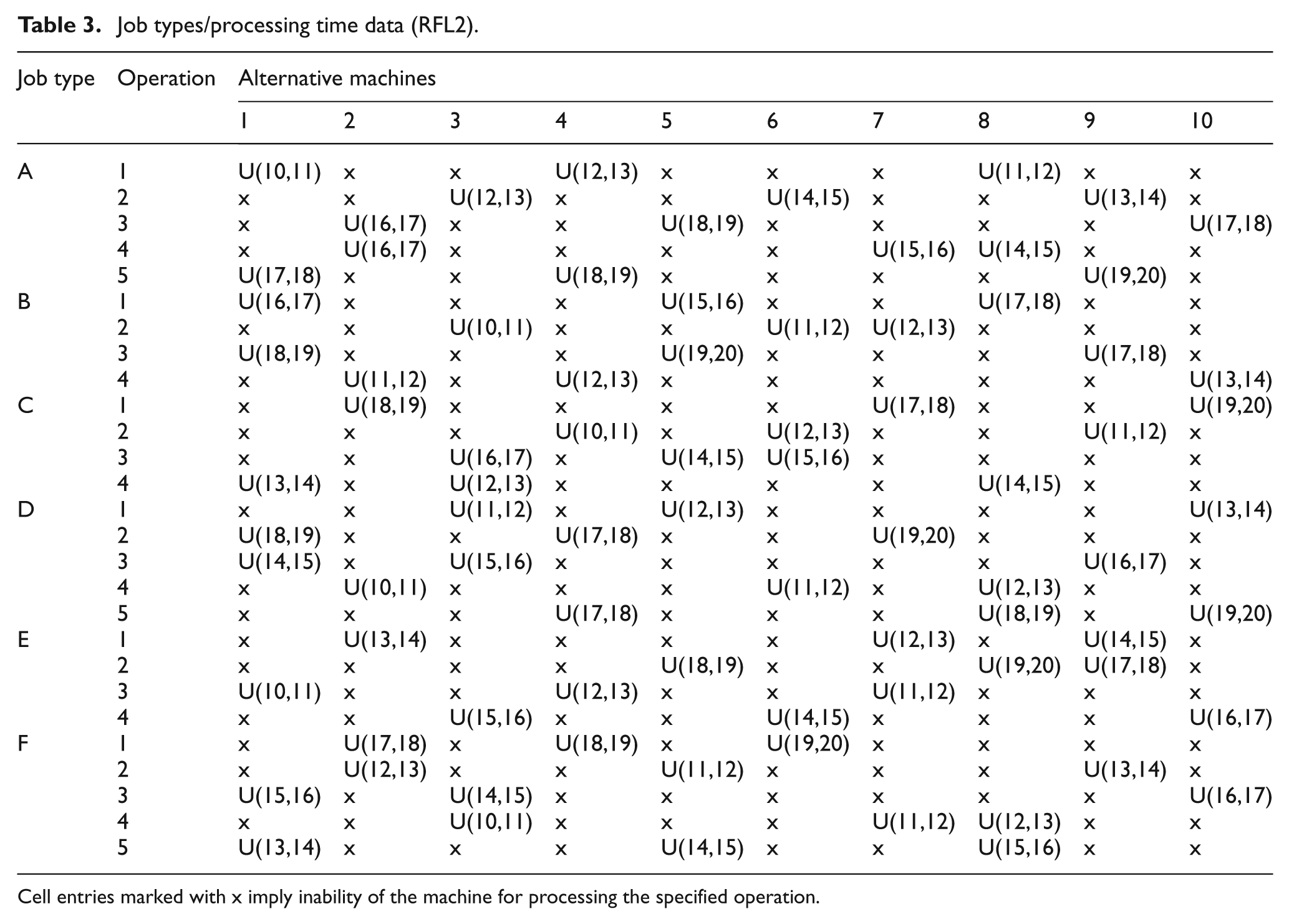
Cell entries marked with x imply inability of the machine for processing the specified operation.

Table 4.

Job types/processing times data (RFL3).

Job type	Operation	Alternative machines
		1	2	3	4	5	6	7	8	9	10
A	1	U(10,11)	x	x	U(12,13)	x	U(11,12)	x	U(11,12)	x	x
	2	U(13,14)	x	U(12,13)	x	x	U(14,15)	x	x	U(13,14)	x
	3	x	U(16,17)	x	x	U(18,19)	x	U(16,17)	x	x	U(17,18)
	4	x	U(16,17)	x	U(14,15)	x	x	U(15,16)	U(14,15)	x	x
	5	U(17,18)	x	x	U(18,19)	U(19,20)	x	x	x	U(19,20)	x
B	1	U(16,17)	x	U(15,16)	x	U(15,16)	x	x	U(17,18)	x	x
	2	x	x	U(10,11)	x	x	U(11,12)	U(12,13)	x	x	U(10,11)
	3	U(18,19)	x	x	x	U(19,20)	x	x	U(19,20)	U(17,18)	x
	4	x	U(11,12)	x	U(12,13)	x	x	x	x	U(13,14)	U(13,14)
C	1	x	U(18,19)	x	x	U(17,18)	x	U(17,18)	x	x	U(19,20)
	2	x	U(10,11)	x	U(10,11)	x	U(12,13)	x	x	U(11,12)	x
	3	U(15,16)	x	U(16,17)	x	U(14,15)	U(15,16)	x	x	x	x
	4	U(13,14)	x	U(12,13)	x	x	x	U(14,15)	U(14,15)	x	x
D	1	x	x	U(11,12)	x	U(12,13)	x	x	U(11,12)	x	U(13,14)
	2	U(18,19)	x	x	U(17,18)	x	x	U(19,20)	x	U(19,20)	x
	3	U(14,15)	x	U(15,16)	x	U(14,15)	x	x	x	U(16,17)	x
	4	x	U(10,11)	x	U(11,12)	x	U(11,12)	x	U(12,13)	x	x
	5	x	U(17,18)	x	U(17,18)	x	x	x	U(18,19)	x	U(19,20)
E	1	x	U(13,14)	U(14,15)	x	x	x	U(12,13)	x	U(14,15)	x
	2	U(18,19)	x	x	x	U(18,19)	x	x	U(19,20)	U(17,18)	x
	3	U(10,11)	x	x	U(12,13)	x	U(12,13)	U(11,12)	x	x	x
	4	x	x	U(15,16)	x	x	U(14,15)	x	U(16,17)	x	U(16,17)
F	1	x	U(17,18)	x	U(18,19)	x	U(19,20)	x	x	U(19,20)	x
	2	x	U(12,13)	x	x	U(11,12)	x	x	U(11,12)	U(13,14)	x
	3	U(15,16)	x	U(14,15)	x	x	x	U(16,17)	x	x	U(16,17)
	4	U(10,11)	x	U(10,11)	x	x	x	U(11,12)	U(12,13)	x	x
	5	U(13,14)	U(15,16)	x	x	U(14,15)	x	x	U(15,16)	x	x

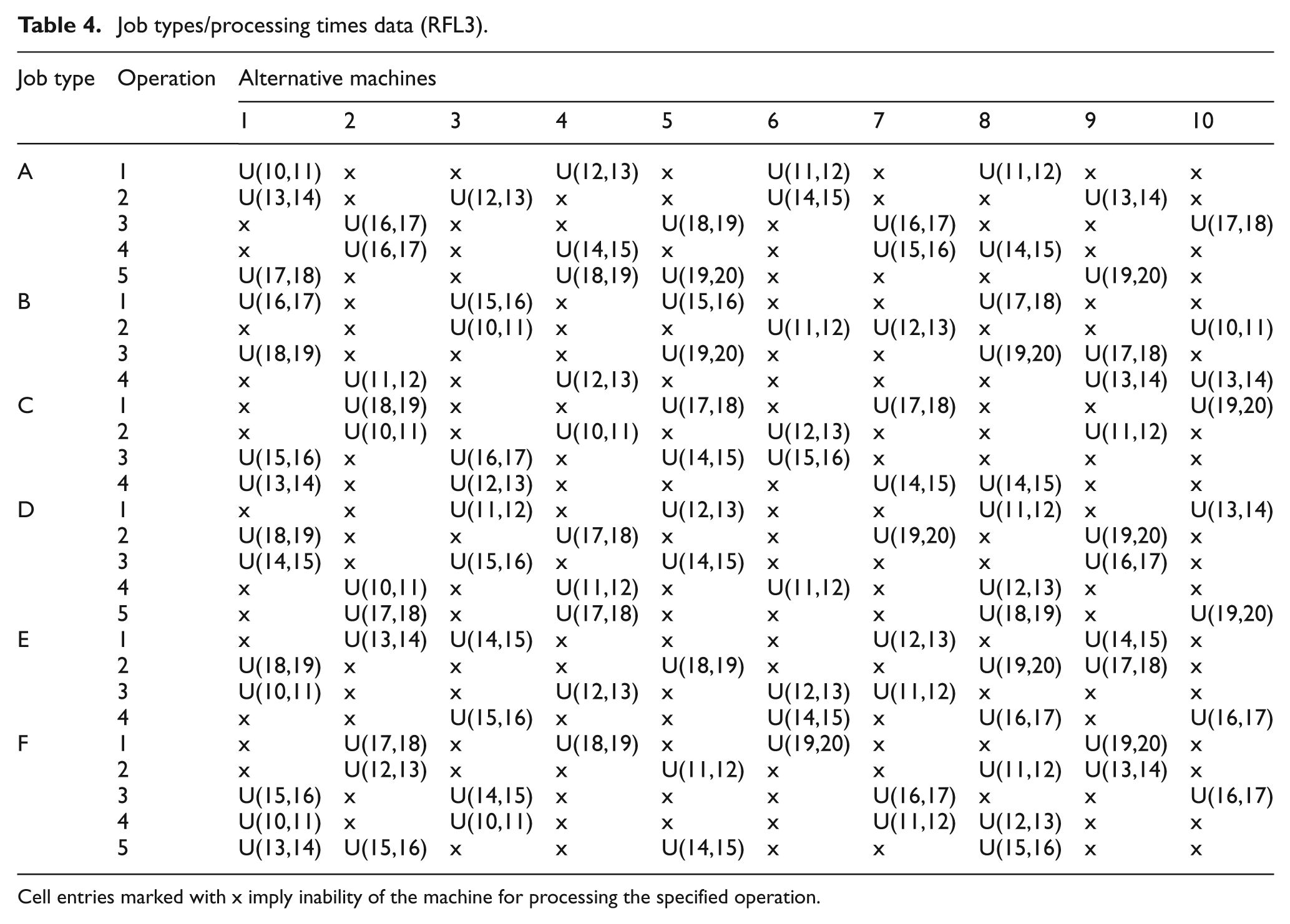
Cell entries marked with x imply inability of the machine for processing the specified operation.

Table 5.

Job types/processing time data (RFL4).

Job type	Operation	Alternative machines
		1	2	3	4	5	6	7	8	9	10
A	1	U(10,11)	x	x	U(12,13)	x	U(11,12)	x	U(11,12)	x	U(13,14)
	2	U(13,14)	x	U(12,13)	x	x	U(14,15)	U(15,16)	x	U(13,14)	x
	3	x	U(16,17)	x	U(19,20)	U(18,19)	x	U(16,17)	x	x	U(17,18)
	4	x	U(16,17)	U(16,17)	U(14,15)	x	x	U(15,16)	U(14,15)	x	x
	5	U(17,18)	x	x	U(18,19)	U(19,20)	U(16,17)	x	x	U(19,20)	x
B	1	U(16,17)	U(19,20)	U(15,16)	x	U(15,16)	x	x	U(17,18)	x	x
	2	U(13,14)	x	U(10,11)	x	x	U(11,12)	U(12,13)	x	x	U(10,11)
	3	U(18,19)	x	x	U(16,17)	U(19,20)	x	x	U(19,20)	U(17,18)	x
	4	x	U(11,12)	x	U(12,13)	x	U(10,11)	x	x	U(13,14)	U(13,14)
C	1	x	U(18,19)	x	x	U(17,18)	x	U(17,18)	U(16,17)	x	U(19,20)
	2	x	U(10,11)	x	U(10,11)	U(13,14)	U(12,13)	x	x	U(11,12)	x
	3	U(15,16)	x	U(16,17)	x	U(14,15)	U(15,16)	x	x	U(13,14)	x
	4	U(13,14)	x	U(12,13)	x	x	x	U(14,15)	U(14,15)	x	U(11,12)
D	1	U(10,11)	x	U(11,12)	x	U(12,13)	x	x	U(11,12)	x	U(13,14)
	2	U(18,19)	U(16,17)	x	U(17,18)	x	x	U(19,20)	x	U(19,20)	x
	3	U(14,15)	x	U(15,16)	x	U(14,15)	x	x	U(13,14)	U(16,17)	x
	4	x	U(10,11)	U(13,14)	U(11,12)	x	U(11,12)	x	U(12,13)	x	x
	5	x	U(17,18)	x	U(17,18)	U(16,17)	x	x	U(18,19)	x	U(19,20)
E	1	x	U(13,14)	U(14,15)	x	U(11,12)	x	U(12,13)	x	U(14,15)	x
	2	U(18,19)	x	x	U(19,20)	U(18,19)	x	x	U(19,20)	U(17,18)	x
	3	U(10,11)	U(13,14)	x	U(12,13)	x	U(12,13)	U(11,12)	x	x	x
	4	U(13,14)	x	U(15,16)	x	x	U(14,15)	x	U(16,17)	x	U(16,17)
F	1	x	U(17,18)	x	U(18,19)	x	U(19,20)	U(16,17)	x	U(19,20)	x
	2	x	U(12,13)	U(10,11)	x	U(11,12)	x	x	U(11,12)	U(13,14)	x
	3	U(15,16)	x	U(14,15)	x	U(17,18)	x	U(16,17)	x	x	U(16,17)
	4	U(10,11)	x	U(10,11)	U(13,14)	x	x	U(11,12)	U(12,13)	x	x
	5	U(13,14)	U(15,16)	x	x	U(14,15)	x	x	U(15,16)	U(12,13)	x

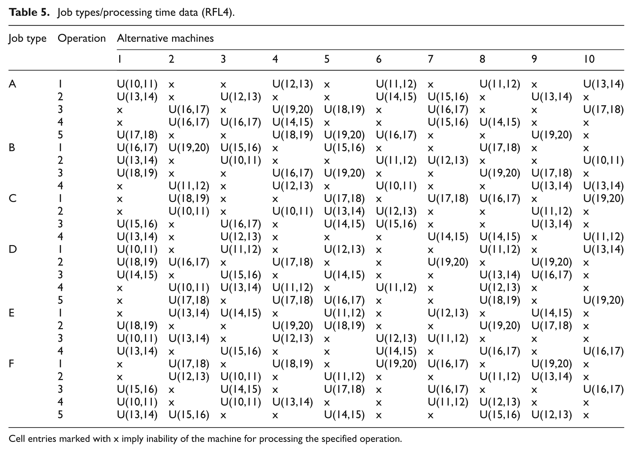
Cell entries marked with x imply inability of the machine for processing the specified operation.

Table 6.

Job types/processing time data (RFL5).

Job type	Operation	Alternative machines
		1	2	3	4	5	6	7	8	9	10
A	1	U(10,11)	U(14,15)	x	U(12,13)	x	U(11,12)	x	U(11,12)	x	U(13,14)
	2	U(13,14)	x	U(12,13)	x	U(15,16)	U(14,15)	U(15,16)	x	U(13,14)	x
	3	x	U(16,17)	x	U(19,20)	U(18,19)	x	U(16,17)	U(15,16)	x	U(17,18)
	4	x	U(16,17)	U(16,17)	U(14,15)	x	x	U(15,16)	U(14,15)	x	U(13,14)
	5	U(17,18)	x	U(15,16)	U(18,19)	U(19,20)	U(16,17)	x	x	U(19,20)	x
B	1	U(16,17)	U(19,20)	U(15,16)	x	U(15,16)	x	x	U(17,18)	U(15,16)	x
	2	U(13,14)	x	U(10,11)	U(14,15)	x	U(11,12)	U(12,13)	x	x	U(10,11)
	3	U(18,19)	U(17,18)	x	U(16,17)	U(19,20)	x	x	U(19,20)	U(17,18)	x
	4	x	U(11,12)	x	U(12,13)	x	U(10,11)	U(12,13)	x	U(13,14)	U(13,14)
C	1	U(15,16)	U(18,19)	x	x	U(17,18)	x	U(17,18)	U(16,17)	x	U(19,20)
	2	x	U(10,11)	U(14,15)	U(10,11)	U(13,14)	U(12,13)	x	x	U(11,12)	x
	3	U(15,16)	x	U(16,17)	x	U(14,15)	U(15,16)	x	U(12,13)	U(13,14)	x
	4	U(13,14)	x	U(12,13)	U(11,12)	x	x	U(14,15)	U(14,15)	x	U(11,12)
D	1	U(10,11)	x	U(11,12)	x	U(12,13)	U(14,15)	x	U(11,12)	x	U(13,14)
	2	U(18,19)	U(16,17)	x	U(17,18)	U(16,17)	x	U(19,20)	x	U(19,20)	x
	3	U(14,15)	x	U(15,16)	x	U(14,15)	x	U(12,13)	U(13,14)	U(16,17)	x
	4	x	U(10,11)	U(13,14)	U(11,12)	x	U(11,12)	x	U(12,13)	x	U(12,13)
	5	U(15,16)	U(17,18)	x	U(17,18)	U(16,17)	x	x	U(18,19)	x	U(19,20)
E	1	x	U(13,14)	U(14,15)	x	U(11,12)	x	U(12,13)	x	U(14,15)	U(11,12)
	2	U(18,19)	x	x	U(19,20)	U(18,19)	U(16,17)	x	U(19,20)	U(17,18)	x
	3	U(10,11)	U(13,14)	x	U(12,13)	x	U(12,13)	U(11,12)	x	U(14,15)	x
	4	U(13,14)	x	U(15,16)	U(12,13)	x	U(14,15)	x	U(16,17)	x	U(13,14)
F	1	x	U(17,18)	x	U(18,19)	x	U(19,20)	U(16,17)	x	U(19,20)	U(15,16)
	2	U(13,14)	U(12,13)	U(10,11)	x	U(11,12)	x	x	U(11,12)	U(13,14)	x
	3	U(15,16)	x	U(14,15)	x	U(17,18)	x	U(16,17)	x	U(17,18)	U(16,17)
	4	U(10,11)	x	U(10,11)	U(13,14)	x	U(11,12)	U(11,12)	U(12,13)	x	x
	5	U(13,14)	U(15,16)	x	U(11,12)	U(14,15)	x	x	U(15,16)	U(12,13)	x

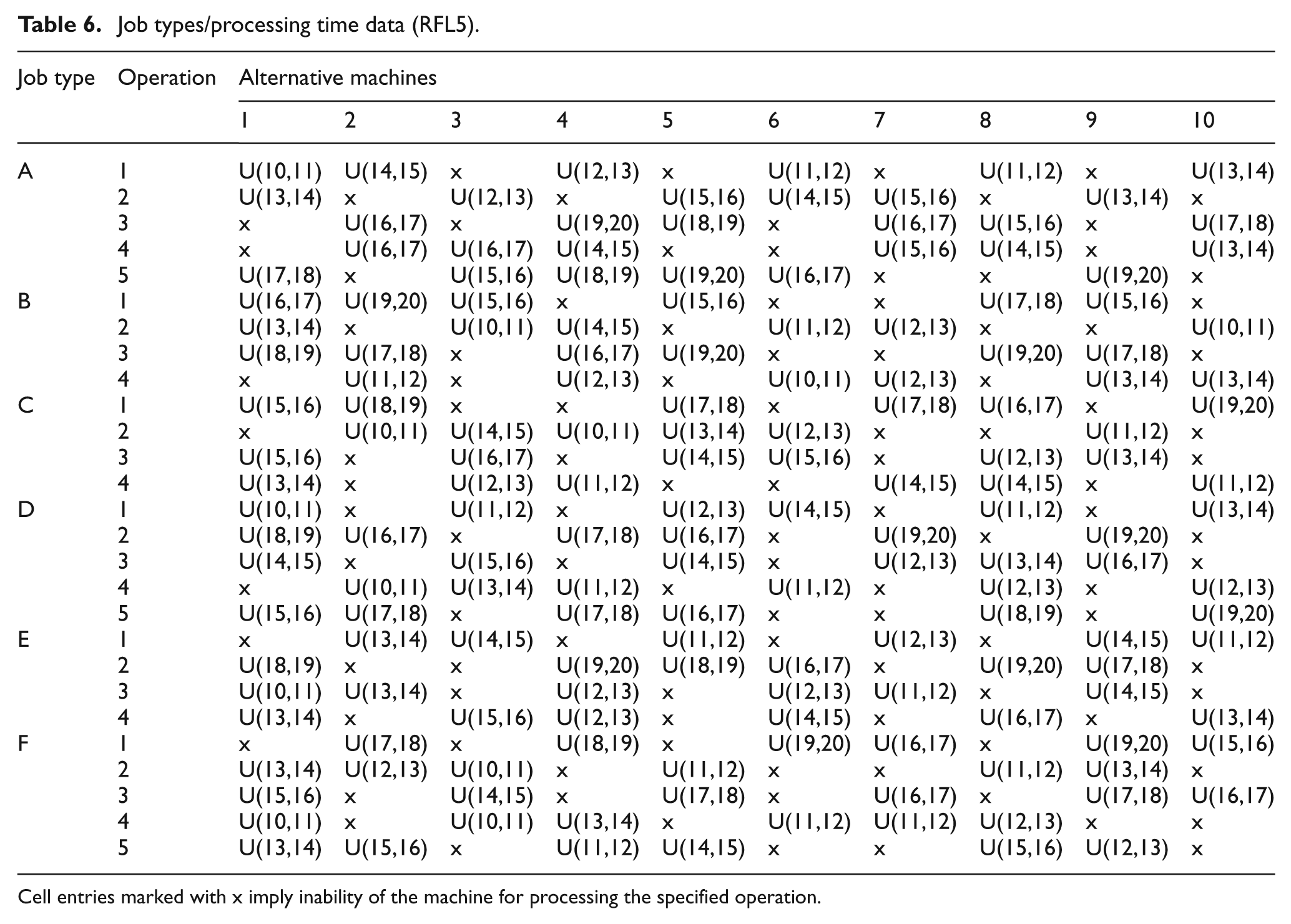
Cell entries marked with x imply inability of the machine for processing the specified operation.

Table 7.

Job types/sequence-dependent setup time data.

Follower job type
Preceding job type	A	B	C	D	E	F
A	0	U(5,5.25)	U(5,5.75)	U(5,5.50)	U(5,5.50)	U(5,5.25)
B	U(5,5.50)	0	U(5,5.25)	U(5,5.75)	U(5,5.25)	U(5,5.50)
C	U(5,5.25)	U(5,5.50)	0	U(5,5.50)	U(5,5.75)	U(5,5.25)
D	U(5,5.75)	U(5,5.25)	U(5,5.50)	0	U(5,5.25)	U(5,5.50)
E	U(5,5.50)	U(5,5.75)	U(5,5.25)	U(5,5.50)	0	U(5,5.25)
F	U(5,5.25)	U(5,5.50)	U(5,5.75)	U(5,5.25)	U(5,5.50)	0

Mean inter-arrival time

It is the average time between arrivals of two jobs. The average arrival rate of jobs must be selected to have utilization of the machine less than 100%. Otherwise, the number of jobs in the queues in front of each machine will grow without bound. ⁵⁷ Thus, the inter-arrival time of the jobs is established using percentage utilization of the shop and processing requirements of the jobs. It has been observed in the literature that the arrival process of the jobs follows a Poisson distribution.^51,57,58 Thus, the inter-arrival time is exponentially distributed. The mean inter-arrival time of the jobs is calculated using the following relationship^35,51

$$b=\frac{1}{\lambda }=\frac{{\mu }_p{\mu }_g}{\mathrm{UM}}$$

(1)

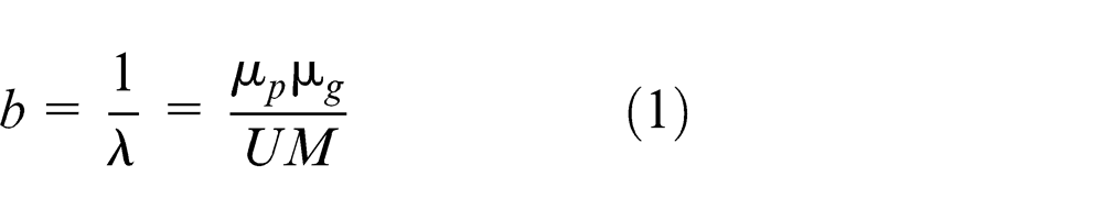
where b = mean inter-arrival time, λ = mean job arrival rate, ${\mu }_p$  = mean processing time per operation (including setup time), ${\mu }_g$  = mean number of operations per job, U = shop utilization and M = number of machines in the shop.

In this work, μ_p is computed by taking the mean of mean processing times of all operations (from Tables 1–6) plus mean of mean setup times (from Table 7). Thus, μ_p = 19.45, 19.45, 19.26, 19.26, 19.21 and 19.10 comes out for RFL0-5, respectively. For the taken input data, μ_g comes out to be 4.5 with M = 10. The experimental study has been carried out at 90% shop utilization, that is, U = 90%.^35,51 Equation (1) reveals that the purpose of shop utilization is to control the inter-arrival time of the jobs. As shop utilization increases, the inter-arrival time of the jobs decreases and the number of jobs in the manufacturing system increases. Furthermore, it is observed that due to the stochastic nature of input processes (processing times and setup times), actual shop load is approximated and falls within a range of ± 1.5% of the target value. ⁵⁹

Due date of jobs

It is the time at which job order must be completed. The due date of the arriving job is either externally or internally determined. In case of externally determined due date, due date is either established by the customer or set for a specific time in the future. In case of internally determined due date, due date is based on the total work content (TWK; sum of processing times and setup times) of the job or number of operations to be performed on the job. Most of the researchers used the TWK method to assign due date of the job^35,51,52,60

$$d_i=a_i+k(p_i+n_i\times u_i)$$

(2)

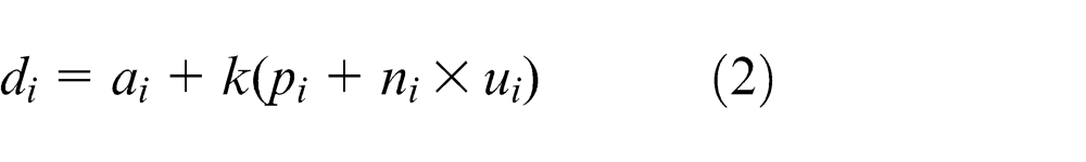
where d_i = due date of job i, a_i = arrival time of job i, k = due date tightness factor, p_i = mean total processing times of all the operations of job i, n_i = number of operations of job i and u_i = mean of mean setup times of all the changeover of job i.

In this study, the due date tightness factor (k) = 3 is considered.

Structure of simulation model

The simulation modelling is one of the most powerful techniques available for studying large and complex manufacturing systems. In this study, a discrete-event simulation model for the operations of the SFJS manufacturing system with different levels of route flexibility and SRLs is developed using PROMODEL software. The job flow in the modelled flexible job shop manufacturing system is shown in Figure 2. The following assumptions are made while developing the simulation model:

1. Each machine can perform at most one operation at a time on any job.

2. An operation cannot start until its predecessor operation is completed.

3. The arrival of jobs in the shop floor is dynamic. A type of job is unknown until it arrives in the shop.

4. Buffer of unlimited capacity is considered before and after each machine.

5. Processing times and setup times are stochastic and known in priori with their distribution.

Figure 2.

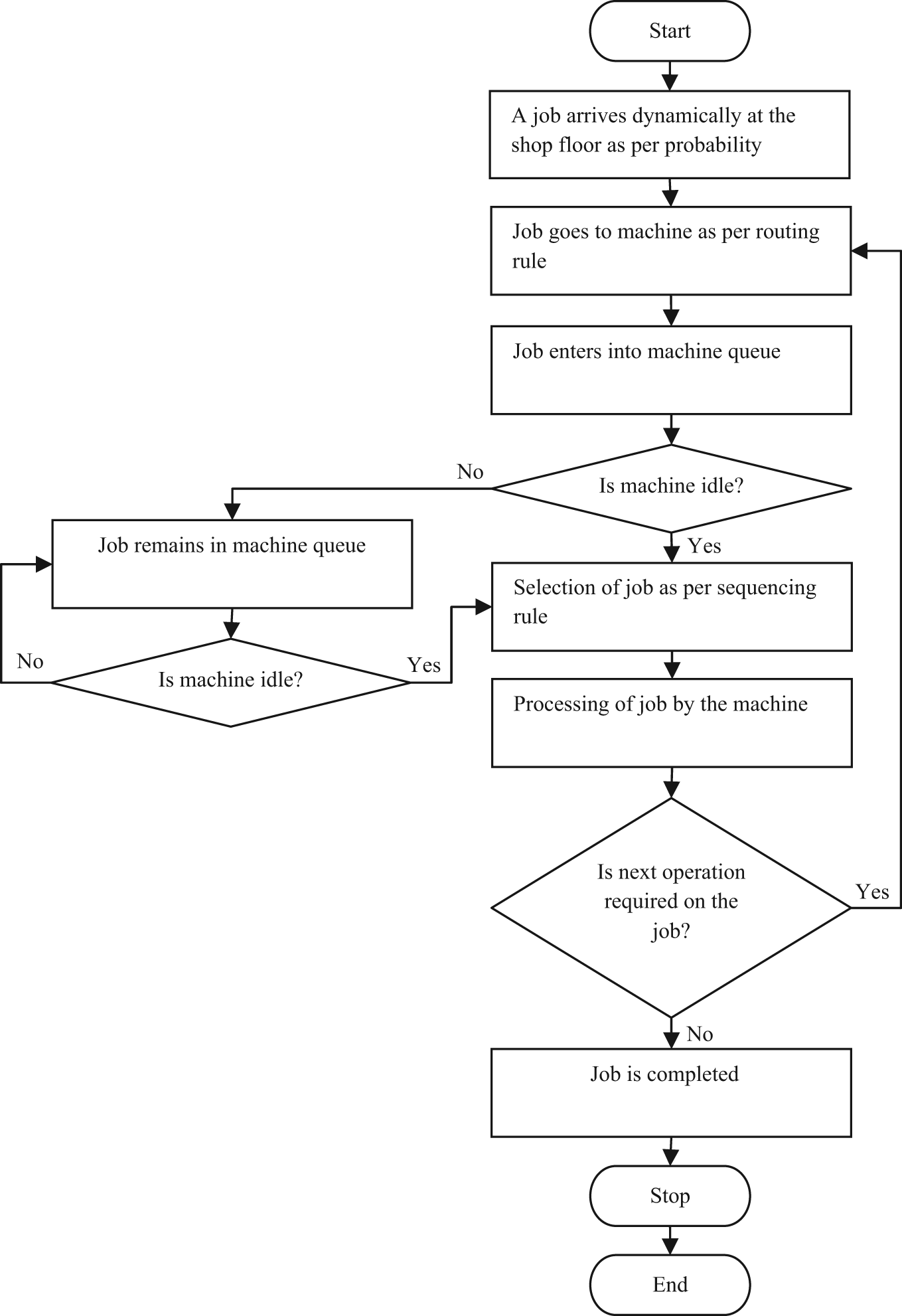
Job flow in the modelled flexible job shop manufacturing system.

Sequencing rules

Sequencing rule is used to select the next job to be processed on the machine from a set of jobs waiting in the input queue of the machine. The following rules as identified from the literature are used for making job sequencing decision:^18,45–50

1. FCFS: The job which arrives first in the input queue of the machine is selected for processing.

2. SPT: The job with shortest processing time for the imminent operation is selected for processing.

3. EDD: The job with earliest due date is selected for processing.

4. SIMSET: The job with shortest setup time for the imminent operation is selected for processing.

5. MWRK: The job with maximum amount of work remaining, that is, having the greatest tail time, is selected for processing.

6. MOPN: The job with maximum numbers of operations remaining is selected for processing.

Routing rule

When a SFJS manufacturing system with routing flexibility is considered, a routing rule is required to select a machine among the set of alternative machines for processing an operation of a job. Joseph and Sridharan ³ reported that out of three routing rules, namely, WINQ (minimum work of jobs in queue), NINQ (minimum number of jobs in queue) and LUM (machine with least utilization), the WINQ rule provides best performance for the measures. Thus, in this work, the WINQ routing rule is taken into consideration. This rule selects a machine among alternative machines whose input queue contains the smallest amount of work, that is, the sum of the processing times of the operations of jobs waiting in the input queue of the machine is minimum.

Performance measures

The following performance measures are used for evaluation purpose in the experimental investigation:

1. Mean flow time ( $\overline{F}$ ): It is the average time that a job spends in the shop during processing

   $$\overline{F}=\frac{1}{n}\left[\sum _{i=1}^n{F}_i\right]$$

   (3)

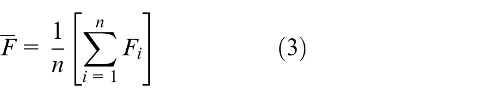
   where F_i = c_i − a_i, F_i = flow time of job i, c_i = completion time of job i, a_i = arrival time of job i and n = number of jobs produced during simulation period (during steady-state period).

2. Maximum flow time (F_max): It is a maximum value of flow time encountered during processing of jobs in the shop

   $$\begin{array}{cc}\multicolumn{1}{c}{}& F_{\max }=\max \left\{F_i\right\}\hfill \\ \multicolumn{1}{c}{}& 1\le i\le n\hfill \end{array}$$

   (4)

3. Mean tardiness ( $\overline{T}$ ): It is the average tardiness of a job in the shop during processing

   $$\overline{T}=\frac{1}{n}\left[\sum _{i=1}^n{T}_i\right]$$

   (5)

   where T_i = max {0, L_i}, L_i = c_i − d_i, T_i = tardiness of job i, L_i = lateness of job i and d_i = due date of job i.

4. Maximum tardiness (T_max): It is a maximum value of tardiness encountered during processing of jobs in the shop

   $$\begin{array}{cc}\multicolumn{1}{c}{}& T_{\max }=\max \left\{T_i\right\}\hfill \\ \multicolumn{1}{c}{}& 1\le i\le n\hfill \end{array}$$

   (6)

5. Number of tardy jobs (TJ): It is the value of the number of jobs which are completed after their due dates

   $$\mathrm{TJ}=\sum _{i=1}^n\delta (T_i)$$

   (7)

   where δ(T_i) = 1 if T_i > 0 and δ(T_i) = 0, otherwise.

Experimental design for simulation study

Using simulation modelling, a number of experiments on SFJS scheduling problem have been conducted. The first stage in simulation experimentation is to identify steady-state period, that is, the end of the initial transient period. Welch’s procedure as described in Law and Kelton ⁶¹ is used for this purpose. A pilot study is conducted for the SFJS scheduling problem, and it is observed that the manufacturing system reaches steady state at the completion of 5000 jobs. A total of 30 replications are considered for simulation experimentation. The simulation for each replication is made to run for 25,000 jobs completion. The jobs are numbered on arrival in the manufacturing system, and simulation outputs from jobs numbering 1–5000 are discarded due to transient period. The outputs for the remaining 20,000 jobs (jobs numbering 5001–25,000) completion are used to compute the different performance measures. Table 8 shows the layout of the SFJS simulation experiments.

Table 8.

Layout of the SFJS simulation experiments.

Machine parameters	Number of machines: 10
	Shop utilization: 90%
Job parameters	Job types: 06
	Number of operations: 4–5
	Mean inter-arrival time: exponential distribution
	Routing pattern: flexible
	Processing times and setup times: stochastic
	Due date: TWK method
Simulation of job shop	Sequencing rules: 06
	Routing rule: 01
	Number of replications: 30
	Run length: 20,000 jobs completion
	(after warm-up period of 5000 jobs)
Performance-related statistics	Performance measures: mean flow time, maximum flow time, mean tardiness, maximum tardiness and number of tardy jobs
	Statistical analysis using ANOVA and LSD test

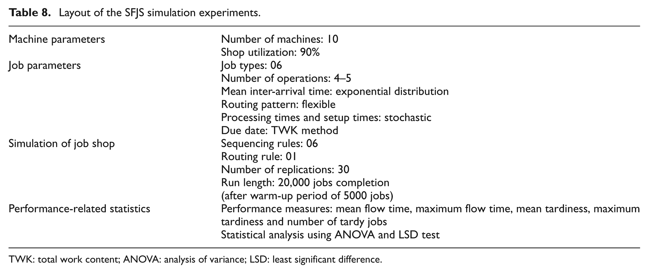
TWK: total work content; ANOVA: analysis of variance; LSD: least significant difference.

The experimental settings of the investigation are summarized in Table 9. The two main control parameters (factors) to be investigated are RFL and SRL. In this connection, 1080 (6 RFLs × 6 SRLs × 30 replications) simulation runs will be performed for the evaluation purpose. The results obtained and their analyses are presented in the following section.

Table 9.

Experimental settings of investigation.

Experimental settings
Route flexibility levels	Sequencing rules	Purpose of investigation
RFL0, RFL1, RFL2, RFL3, RFL4 and RFL5	FCFS, SPT, EDD, SIMSET, MWRK and MOPN	Analyse the effect of different levels of route flexibility and sequencing rules on the stochastic flexible job shop manufacturing system performance

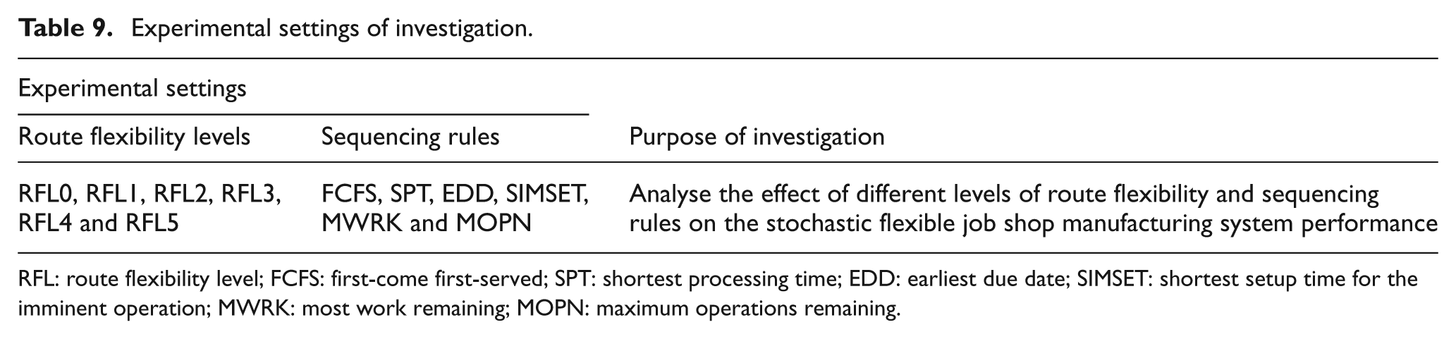
RFL: route flexibility level; FCFS: first-come first-served; SPT: shortest processing time; EDD: earliest due date; SIMSET: shortest setup time for the imminent operation; MWRK: most work remaining; MOPN: maximum operations remaining.

Simulation results and analyses

In this research work, two different studies are carried out using simulation results. In the first study, the average values of the performance measures for each simulation experiment are analysed using graphical plots.

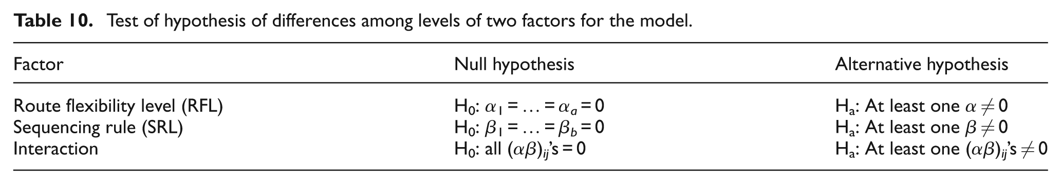
In the second study, the effect of RFLs and SRLs on SFJS manufacturing system performance is assessed. Since RFL and SRL are two main factors, the interaction between the two factors and which factor has more significant effect on the performance of SFJS manufacturing system are analysed using two-factor analysis of variance (ANOVA) F-test. The null hypothesis and the alternative hypothesis for the ANOVA F-test are provided in Table 10. The least significant difference (LSD) method is used for performing pairwise comparisons in order to determine the means that differ from other means. The values that are not significantly different are grouped together. All the tests are performed at 5% significance level.

Table 10.

Test of hypothesis of differences among levels of two factors for the model.

Factor	Null hypothesis	Alternative hypothesis
Route flexibility level (RFL)	H0: α1 = … = α a  = 0	Ha: At least one α ≠ 0
Sequencing rule (SRL)	H0: β1 = … = β b  = 0	Ha: At least one β ≠ 0
Interaction	H0: all (αβ) ij ’s = 0	Ha: At least one (αβ) ij ’s ≠ 0

Graphical analyses of means

For each performance measure at different RFLs and SRLs, the simulation output of 30 replications is averaged. The average values of performance measures are presented in Figures 3–7. The performance measure values at RFL1, RFL2 and RFL3 appear to be flat because of the small difference in their values and lower values as compared to RFL0.

Figure 3.

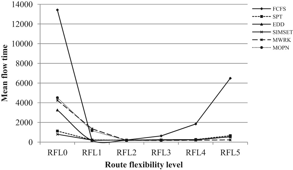
Comparing mean flow time of sequencing rules at different route flexibility levels.

Figure 4.

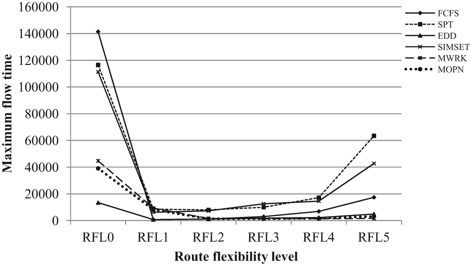
Comparing maximum flow time of sequencing rules at different route flexibility levels.

Figure 5.

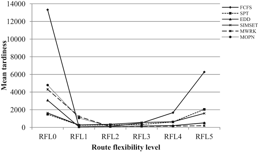
Comparing mean tardiness of sequencing rules at different route flexibility levels.

Figure 6.

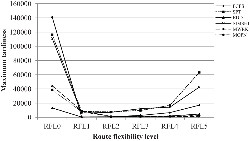
Comparing maximum tardiness of sequencing rules at different route flexibility levels.

Figure 7.

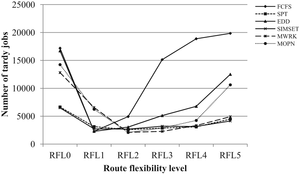
Comparing number of tardy jobs of sequencing rules at different route flexibility levels.

Mean flow time

Figure 3 shows simulation results for mean flow time for various combinations of RFLs and SRLs. At RFL1, the due date–based SRL, that is, EDD provides the minimum value for this performance measure. The FCFS and SIMSET rules provide the values close to those of EDD rule at the same RFL. At RFL2, MOPN and SPT SRLs provide the best results. The performance measure values of MOPN and SPT SRLs are close to each other. At higher RFL, that is, RFL3, the MWRK rule provides the best performance. Thus, when routing flexibility is present in the system, the EDD rule at RFL1 is the best performing SRL for the mean flow time performance measure.

Maximum flow time

Figure 4 shows simulation results for the maximum flow time performance measure at different pairs of RFLs and SRLs. At RFL1, the EDD SRL provides the minimum value for this performance measure. At the same RFL, the FCFS rule provides the value close to that of EDD rule, but the SIMSET rule provides a very large value. The MOPN and SPT SRLs provide the best performance at RFL2. The MOPN rule provides smaller value as compared with the SPT rule. The MWRK rule works well at RFL4. Here also, the EDD rule at RFL1 dominates all other SRLs.

Mean tardiness

Figure 5 compares the mean tardiness performance measure at different RFLs and SRLs. At RFL1, the EDD SRL provides the minimum value for the mean tardiness. At the same RFL, the FCFS rule provides the value close to that of the EDD rule, while the SPT and SIMSET rules provide very large values. At RFL2, the MOPN and MWRK rules provide the best performance. The performance measure values of both SRLs are close to each other. For this performance measure, the EDD rule at RFL1 is the best performing SRL.

Maximum tardiness

Figure 6 shows simulation results for the maximum tardiness performance measure at different combinations of RFLs and SRLs. At RFL1, the EDD SRL provides the best performance. A similar pattern is observed for FCFS and SIMSET SRLs. At RFL1, the FCFS rule provides the value close to that of the EDD rule, while the SIMSET rule provides a very large value. The MOPN and SPT rules provide the best performance at RFL2. The MOPN SRL provides a smaller value as compared with the SPT rule. The MWRK rule works well at higher RFL, that is, RFL4. The EDD rule at RFL1 dominates all other SRLs for the maximum tardiness performance measure.

Number of tardy jobs

Figure 7 compares the number of tardy jobs performance measure at different RFLs and SRLs. At RFL1, the EDD SRL provides the minimum value. The FCFS rule also works well at the same RFL and provides the second lowest value. All other SRLs provide the best performance at RFL2. At this RFL, the MOPN rule provides the minimum value, while the SIMSET rule provides the maximum value. For this performance measure, the EDD rule at RFL1 is the best performing SRL.

For each SRL, the relative percentage improvement (RPI) in each performance measure at each RFL (RFL1, RFL2, RFL3, RFL4 and RFL5) is calculated relative to RFL0. For example, the RPI of the mean flow time ( $\overline{F}$ ) for the FCFS rule at RFL1 is calculated as follows

$$\begin{array}{c}\multicolumn{1}{c}{\mathrm{RPI}\mathrm{for}\overline{F}\_\mathrm{FCFS}\_\mathrm{RFL}1}\\ \multicolumn{1}{c}{=\frac{(\overline{F}\_\mathrm{FCFS}\_\mathrm{RFL}0-\overline{F}\_\mathrm{FCFS}\_\mathrm{RFL}1)}{\overline{F}\_\mathrm{FCFS}\_\mathrm{RFL}0}\times 100}\end{array}$$

(8)

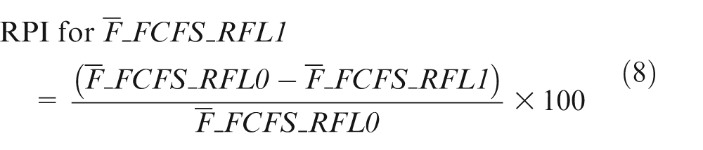
For the FCFS SRL,

• Value of mean flow time at RFL0 ( $\overline{F}$ _FCFS_RFL0) = 13,430.00;

• Value of mean flow time at RFL1 ( $\overline{F}$ _FCFS_RFL1) = 179.64.

By using equation (8), the RPI for $\overline{F}$ _FCFS_RFL1 comes out to be 98.66. Similarly for each SRL, the RPI in each performance measure at each RFL is calculated. The RPI values for different performance measures are shown in Table 11.

Table 11.

RPI in performance measures under different sequencing rules.

Sequencing rule	Performance measure	RPI
		RFL1	RFL2	RFL3	RFL4	RFL5
FCFS	$\overline{F}$	98.66	98.41	95.31	86.28	51.71
	Fmax	99.45	99.20	97.89	95.12	87.68
	$\overline{T}$	99.50	99.08	96.27	87.49	52.92
	Tmax	99.64	99.38	98.07	95.29	87.85
	TJ	86.70	71.34	11.93	09.83	15.47
SPT	$\overline{F}$	80.79	82.16	80.95	76.76	41.54
	Fmax	92.69	93.14	91.44	85.28	45.50
	$\overline{T}$	83.38	81.71	77.75	58.53	37.51
	Tmax	92.88	93.38	91.67	85.50	45.65
	TJ	53.03	60.92	56.83	53.61	32.75
EDD	$\overline{F}$	94.68	94.51	93.39	92.18	83.26
	Fmax	94.45	91.50	86.51	83.51	63.62
	$\overline{T}$	98.06	96.95	95.16	93.48	83.39
	Tmax	96.46	93.40	88.39	85.33	65.06
	TJ	86.35	81.75	69.40	59.50	25.19
SIMSET	$\overline{F}$	74.98	74.50	68.85	67.46	33.23
	Fmax	94.40	93.47	88.76	86.93	61.59
	$\overline{T}$	83.00	78.18	65.87	61.09	02.40
	Tmax	94.59	93.67	88.95	87.11	61.72
	TJ	57.85	58.77	50.55	51.38	36.27
MWRK	$\overline{F}$	68.19	95.93	95.96	95.55	94.67
	Fmax	79.07	96.61	96.75	96.93	96.36
	$\overline{T}$	71.36	97.78	97.25	96.84	95.64
	Tmax	79.54	97.11	97.26	97.46	96.91
	TJ	48.81	83.58	82.22	74.05	61.73
MOPN	$\overline{F}$	74.35	96.21	95.93	95.16	88.15
	Fmax	79.00	96.54	96.45	95.59	91.90
	$\overline{T}$	77.93	98.07	97.23	96.34	89.86
	Tmax	79.52	97.16	97.04	96.17	92.53
	TJ	56.16	85.35	79.79	70.23	25.42

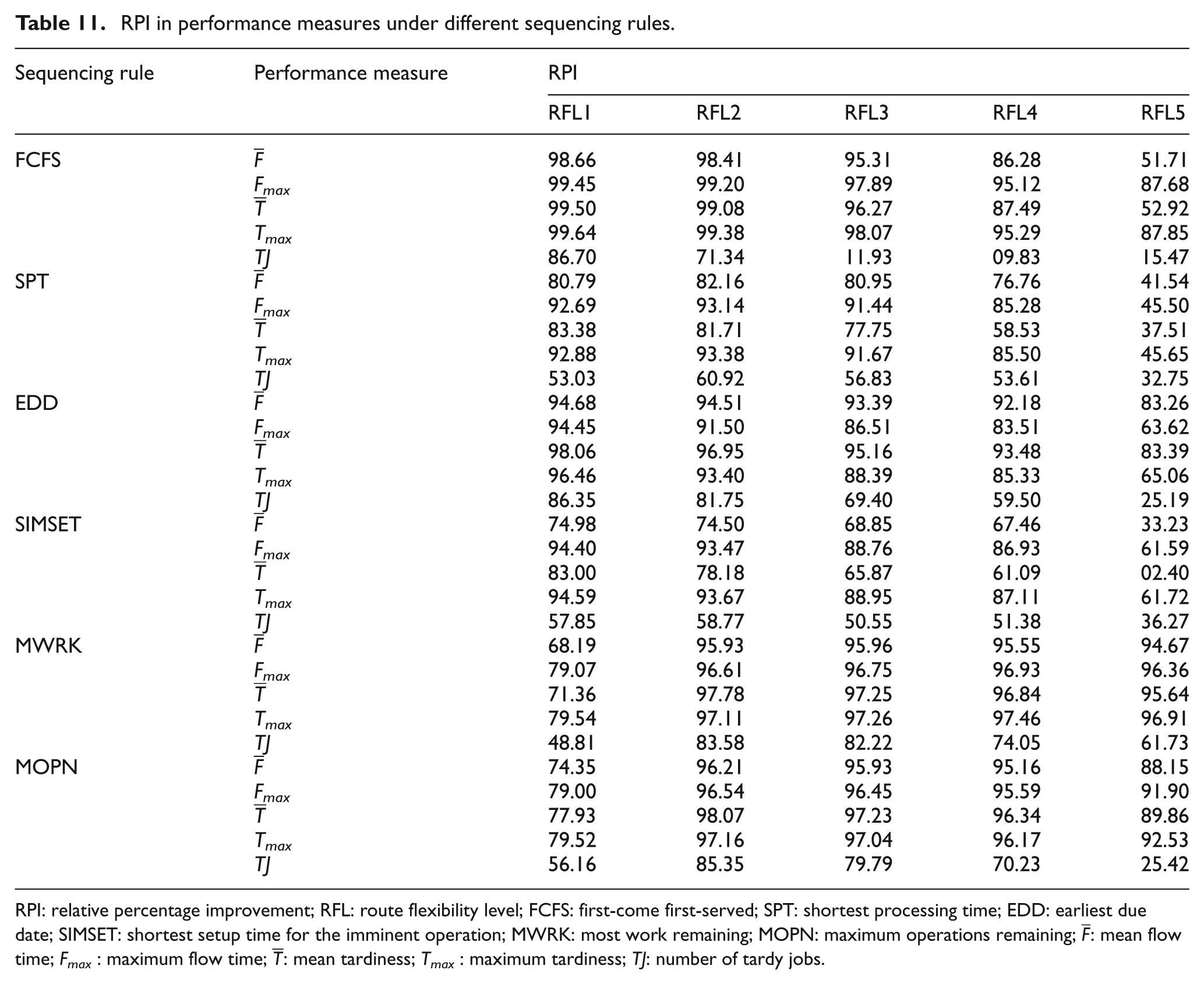
RPI: relative percentage improvement; RFL: route flexibility level; FCFS: first-come first-served; SPT: shortest processing time; EDD: earliest due date; SIMSET: shortest setup time for the imminent operation; MWRK: most work remaining; MOPN: maximum operations remaining; $\overline{F}$ : mean flow time; F_max : maximum flow time; $\overline{T}$ : mean tardiness; T_max : maximum tardiness; TJ: number of tardy jobs.

From the above illustrations and Table 11, it is evident that the beneficial effects of routing flexibility with each SRL can be observed for all the performance measures but up to certain levels of route flexibility. When route flexibility is increased beyond those particular levels, the system performance deteriorates. It is also observed that at RFL1, there is a drastic decrease in RPI values of all the performance measures for the FCFS SRL.

Statistical analysis

The simulation results of 30 replications of 36 experiments are used to conduct two-factor ANOVA F-test. The results of the statistical test are shown in Table 12.

Table 12.

ANOVA results

Source of variation (Factor)	F-ratio for performance measures
	$\overline{F}$	Fmax	$\overline{T}$	Tmax	TJ
Main effect
A: RFL	2931.23 a	1065.37 a	2583.75 a	1065.20 a	3133.68 a
B: SRL	1694.79 a	252.26 a	1061.82 a	252.27 a	2967.39 a
Interaction effect: AB	629.04 a	94.19 a	477.88 a	94.16 a	461.32 a

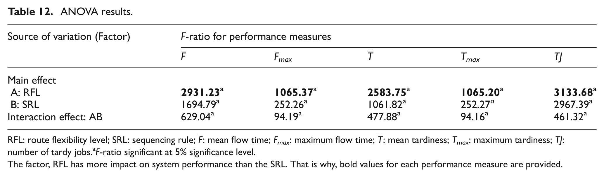
RFL: route flexibility level; SRL: sequencing rule; $\overline{F}$ : mean flow time; F_max: maximum flow time; $\overline{T}$ : mean tardiness; T_max: maximum tardiness; TJ: number of tardy jobs.

a

F-ratio significant at 5% significance level. The factor, RFL has more impact on system performance than the SRL. That is why, bold values for each performance measure are provided.

The main effects, namely, RFL and SRL, are found to be statistically significant at 5% significance level for all the performance measures as the probability value (p-value) for the F-test comes out to be 0.00 (less than 0.05). The F-ratio values for the RFL are larger than those for the SRL. It means that the factor RFL has more impact on system performance than the SRL. Furthermore, the interaction effects are also found to be statistically significant for all the performance measures.

The effect of routing flexibility

Fisher’s LSD method of pairwise multiple comparisons is used to determine the levels of route flexibility that are statistically significant. Table 13 provides the results obtained using LSD test for RFLs. Since there is significant difference between different levels of route flexibility for the number of tardy jobs performance measure, each RFL forms a unique significant group labelled ‘a’, ‘b’, ‘c’, ‘d’, ‘e’ and ‘f’. For mean flow time and mean tardiness performance measures, there is no significant difference between RFL1 and RFL4; hence, these two levels form a unique group labelled ‘b’. RFL0, RFL2, RFL3 and RFL5 form unique group labelled ‘a’, ‘c’, ‘d’ and ‘e’, respectively. Five groups labelled ‘a’, ‘b’, ‘c’, ‘d’ and ‘e’ are formed for maximum flow time and maximum tardiness performance measures. Although there is no statistically significant difference between RFL1 and RFL4 for mean flow time, maximum flow time, mean tardiness and maximum tardiness performance measures, RFL1 provides better performance than the RFL4.

Table 13.

Multiple comparison test results (main effect – RFL).

RFL	$\overline{F}$	Fmax	$\overline{T}$	Tmax	TJ
RFL0	4562.25a	77,743.51a	4770.56a	77,473.39a	12,352.59a
RFL1	546.29b	5640.58b	490.29b	5382.50b	3871.41b
RFL2	189.92 c	3398.40 b,e	171.71 c	3142.49 b,e	2907.85 c
RFL3	276.82d	5019.58b	297.13d	4762.98b	5249.47d
RFL4	504.28b	7318.34b,c	571.47b	7059.60b,c	6575.19e
RFL5	1497.70e	22,221.64d	1848.28e	21,964.39d	9415.91f

$\overline{F}$ : mean flow time; F_max : maximum flow time; $\overline{T}$ : mean tardiness; T_max: maximum tardiness; TJ: number of tardy jobs; LSD: least significant difference.

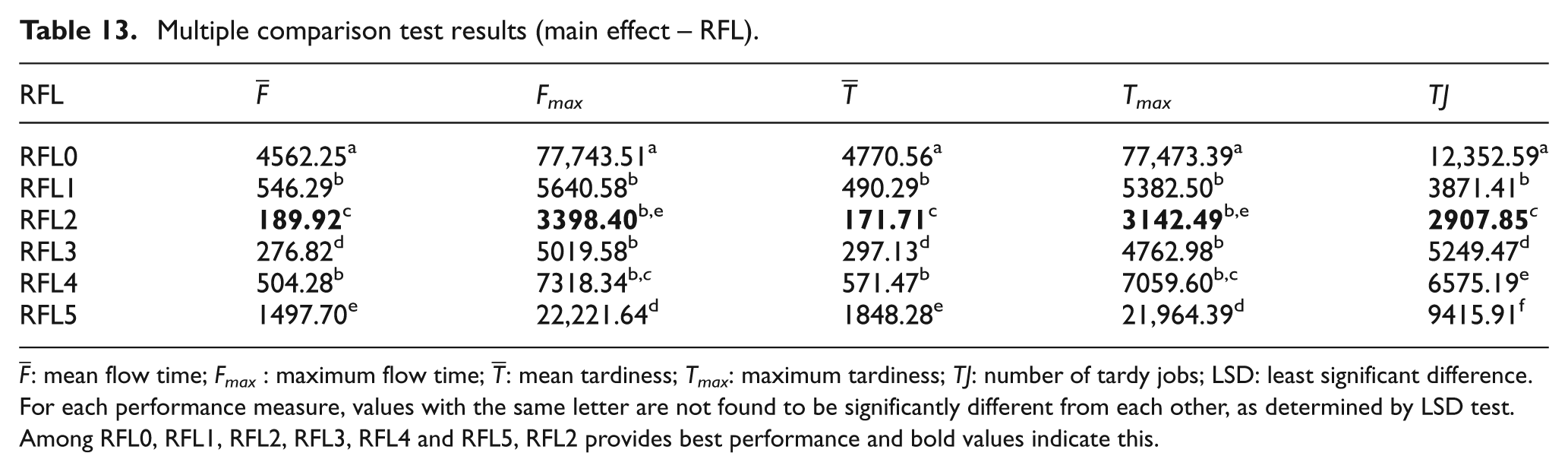
For each performance measure, values with the same letter are not found to be significantly different from each other, as determined by LSD test. Among RFL0, RFL1, RFL2, RFL3, RFL4 and RFL5, RFL2 provides best performance and bold values indicate this.

Thus, it is evident from Table 13 that the RFLs have a significant effect on the system performance. As expected, all the performance measures have higher values at RFL0 compared with that obtained when routing flexibility is present in the system. For all the measures, RFL2 provides the best performance when mean values of all the SRLs are compared. Beyond this RFL, the system performance starts to deteriorate and becomes worst at RFL5.

The effect of SRLs

Table 14 shows the effect of SRLs on the performance of the manufacturing system. For the mean flow time performance measure, there is no significant difference between SPT and SIMSET SRLs, so these rules form a unique group labelled ‘b’. The MWRK and MOPN SRLs also form a unique group labelled ‘d’. The other SRLs, namely, FCFS and EDD, form separate unique group labelled ‘a’ and ‘c’, respectively. For maximum flow time and maximum tardiness performance measures, MWRK and MOPN SRLs form a unique group labelled ‘e’. The other rules such as FCFS, SPT, EDD and SIMSET form separate unique group labelled ‘a’, ‘b’, ‘c’ and ‘d’, respectively. For mean tardiness and number of tardy jobs performance measures, SPT and SIMSET SRLs form a unique group labelled ‘b’. The FCFS, EDD, MWRK and MOPN rules form unique separate group labelled ‘a’, ‘c’, ‘d’ and ‘e’, respectively.

Table 14.

Multiple comparison test results (main effect – SRL).

SRL	$\overline{F}$	Fmax	$\overline{T}$	Tmax	TJ
FCFS	3797.45a	28,443.23a	3661.07a	28,170.34 a	13,052.94a
SPT	445.91b	37,270.38b	831.96b	37,003.58b	3802.45b
EDD	771.40c	4042.72 c	682.03c	3771.04 c	7738.72c
SIMSET	371.80 b	32,437.39d	838.62b	32,182.80d	3735.39 b
MWRK	1060.86d	10,017.93e	1013.93d	9754.09e	5330.46d
MOPN	1131.34d	9149.68e	1123.45e	8890.26e	6718.59e

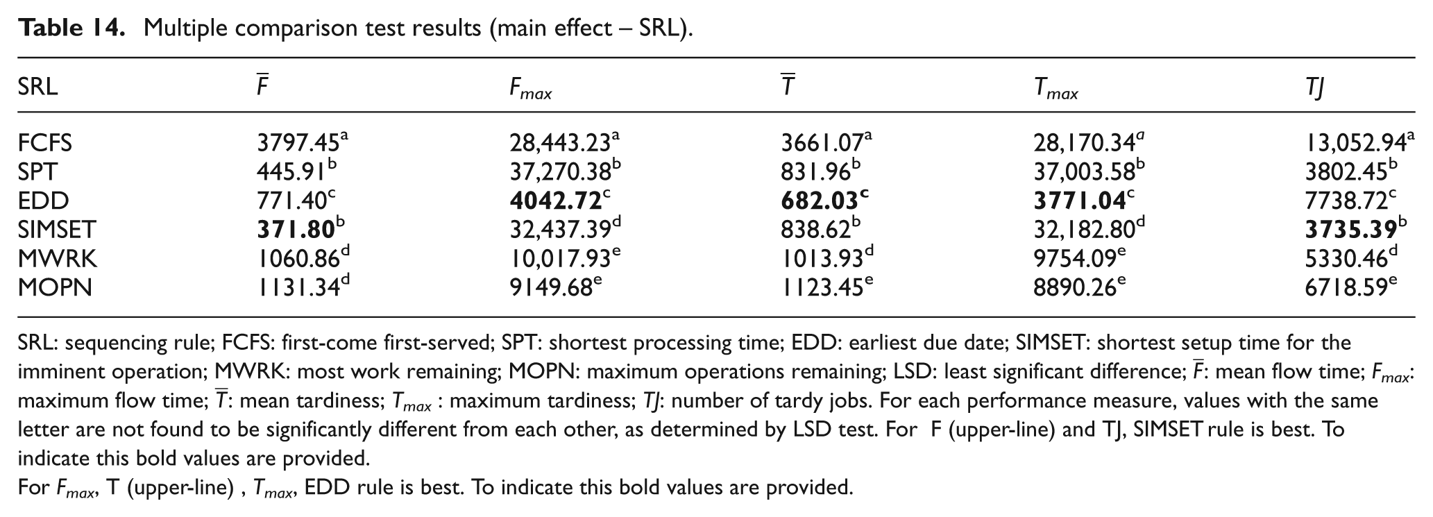
SRL: sequencing rule; FCFS: first-come first-served; SPT: shortest processing time; EDD: earliest due date; SIMSET: shortest setup time for the imminent operation; MWRK: most work remaining; MOPN: maximum operations remaining; LSD: least significant difference; $\overline{F}$ : mean flow time; F_max: maximum flow time; $\overline{T}$ : mean tardiness; T_max : maximum tardiness; TJ: number of tardy jobs.

For each performance measure, values with the same letter are not found to be significantly different from each other, as determined by LSD test. For F (upper-line) and TJ, SIMSET rule is best. To indicate this bold values are provided.For F_max, T (upper-line) , T_max, EDD rule is best. To indicate this bold values are provided.

It is evident from Table 14 that among all the SRLs considered in this study, the EDD SRL is found to provide best performance for maximum flow time, mean tardiness and maximum tardiness measures, whereas the SIMSET rule provides best performance for mean flow time and number of tardy jobs measures. Thus, the SRLs have a significant effect on the system performance.

Conclusion

In this study, the effect of routing flexibility and SRLs on the performance of SFJS manufacturing system with sequence-dependent setup times has been analysed using a discrete-event simulation model. The statistical analysis of the simulation results reveals that the two factors, RFL and SRL, are statistically significant. There is a significant interaction between levels of route flexibility and SRLs for all the performance measures. The results can be summarized as follows:

1. Without having the presence of routing flexibility in the manufacturing system, that is, RFL0, all the performance measures have higher values.

2. By incorporating routing flexibility up to RFL2, there is great improvement in performance measure values. However, beneficiary effects start to diminish as the levels of route flexibility are further increased. At higher RFL, that is, RFL5, the system performance becomes worst. Thus, increasing routing flexibility cannot be treated as a key role in system improvement.

3. The due date–based SRL such as EDD provides best performance for maximum flow time, mean tardiness and maximum tardiness measures. The SIMSET rule outperforms all other SRLs for mean flow time and number of tardy jobs performance measures.

4. For all the performance measures, F-ratio values for the factor RFL are more than those of the SRL. Thus, the routing flexibility has more impact on system performance than the SRLs.

This work indicates that by incorporating routing flexibility, there is reduction in flow time–related performance measures which results in the reduction of average inventory and improved manufacturing lead time. All due date–related performance measures are also reduced. This results in better customer service and satisfaction. This work can be extended in several ways. Further experimental work is required to assess the effect of routing flexibility on SFJS manufacturing system performance with setup times involving situations like limited capacity buffer between machines, machine breakdown, batch mode schedule and external disturbances such as order cancellation and job pre-emption. The work can also be extended to assess the effect of different shop utilization percentage as well as due date tightness factor. Furthermore, the development of new SRLs and routing rules is required that can perform better than the existing rules. These studies will assist in improving the understanding of flexible job shop manufacturing system performance so that manufacturing manager can control it in efficient manner.