Theoretical modeling of tool mean temperature during ultrasonically assisted turning

Abstract

This article summarizes the results of theoretical and experimental studies of average tool temperature in ultrasonic-assisted turning of aerospace aluminum using Al₂O₃-coated tools. In theoretical study, thermal modeling of heat source at the tool–work interface and the temperature distribution in the cutting tool are presented. To determine the actual performance, the sticking and slipping tool–chip contact lengths (l_c and l_s) are experimentally measured and then heat source at the tool–work interface is modeled according to the analogy between shear stress distribution and heat source distribution on the rake face. Then, with respect to the kinematics of the process, the cutting velocity model is presented. The velocity model is used to define the heat flux equation and shear strain rate in ultrasonic-assisted turning. Using heat flux function and Johnson–Cook model, the temperature distribution in a semi-infinite rectangular corner, as a function of time and distance from tool tip, is presented. The analysis results are compared with experimental measurements of average cutting temperature from ultrasonic-assisted turning tests on 7075 aluminum using K-type Testo 735 thermocouple. On the other hand, results show that ultrasonic-assisted turning does not necessarily lower the average cutting temperature in all cases. The effectiveness of the technique is highly dependent on the value of vibration amplitude, work velocity, and feed rate. At low feed rates and amplitudes, the average tool temperature for ultrasonic-assisted turning is 60% of the conventional turning value while growing with an increase in feed rate and amplitude.

Introduction

Ultrasonic-assisted turning (UAT) adds low amplitude and high-frequency displacement to the cutting motion of the tool. The cutting tool is driven harmonically in a linear path, which is superimposed on the cutting motion of the workpiece. This situation is called one-dimensional (1D) UAT (Figure 1). Two-dimensional (2D) UAT adds vertical harmonic motion to the horizontal motion of 1D. The benefits of UAT (such as increasing tool life, improving surface finish, and lower cutting forces) derive the periodic separation of the tool rake face from the uncut material and have been attributed to the 1D and 2D mode technology. ¹

Figure 1.

A scheme of relative movements of workpiece and cutting tool in 1D UAT.

The importance of temperature measurement and its prediction in machining processes have been well recognized. ² It strongly influences tool life, tool wear, tool fracture, and residual thermal stresses. UAT has the ability to reduce the tool wear significantly, which leads to improve cooling conditions and reduces tool tip temperature. ²

Up to now several theories have been presented concerning the explanation of this phenomenon. Some suggest that the performance is due to the coolant effects, either convective heat transfer or actually pumping liquid coolant into the interface. ³ Some suggest that the friction on the tool is the main contributor to decrease the amount of heat generated. ⁴ Others believe that cutting tool is machining for less time as compared with constant cutting; therefore, of course, tool temperature will decrease. ¹

Despite previous researches, thermal aspects of this process have not been fully understood and further researches are required. On the other hand, it is not possible to experimentally determine the influence of many of the variables on the cutting temperature or to measure conveniently its components. It is necessary to develop models to evaluate the cutting temperature in UAT process either analytically or numerically. Therefore, this article is dedicated to the theoretical and experimental study of mean tool temperatures in UAT process, and additional consideration is given to the UAT cutting mechanism and how it may reduce cutting temperature.

Literature review

The history of cutting temperature research in Conventional Turning (CT) goes back as far as Taylor’s experimental works in 1907. Trigger and Chao ⁵ made the first attempt to evaluate the cutting temperature analytically. Usui et al. ⁶ and Tlusty and Orady ⁷ used the finite difference method to predict the steady-state temperature distribution in turning. Strenkowski and Moon ⁸ have developed an Eulerian finite element model to simulate the cutting temperature. Stephenson and Ali ⁹ analyzed a special case of interrupted cutting with constant chip thickness. Ren and Altintas ¹⁰ applied a slip line field solution on high-speed orthogonal turning of hardened mold steels. Lazoglu and Altintas ¹¹ used finite difference method for the predictions of steady-state tool and chip temperature fields and transient temperature variation in continuous machining and milling.

Mitrofanov et al. ¹² used MSC Marc/Mentat general FE code and provided finite element simulations of ultrasonically assisted turning. These authors ¹³ presented a 2D finite element model of ultrasonically assisted turning for a nickel-based alloy Inconel 718 and reported a decrease in cutting forces and working temperatures as well as a superior surface finish. In another work, they also developed a 3D model used for transient, coupled thermo mechanical simulations of elasto-plastic materials under conditions of both UAT and CT. ¹⁴ Numerical results were also validated by experimental tests. Amini et al. ¹⁵ used MSC Marc and ANSYS and studied machining of Inconel 738 with a tool vibrating at ultrasonic frequency. Overcash and Cuttino ¹⁶ developed a model used to describe the mechanism by which vibration-assisted machining reduces tool temperature, and correlations to resulting reduction in tool wear were presented. Finally, Muhammad et al. ¹⁷ developed a three-dimensional finite element model for both conventional and ultrasonically assisted turning techniques in a commercial code MSC Marc/Mentat.

The review confirms that despite a significant amount of research, there has been no major analytical study on temperature distribution during UAT. Therefore, this article is dedicated to analytical study of cutting tool temperature during UAT.

In order to do so, the kinematics of the process is studied and cutting velocity model is developed. This velocity model is used to define the heat flux function and shear strain rate in UAT. Then sticking and slipping tool–chip contact lengths (l_c and l_s) are experimentally measured, and heat flux function at the tool–work interface is modeled according to the analogy between shear stress distribution and heat source distribution on the rake face. In continuation, workpiece material is modeled using Johnson–Cook (JC) constitutive model. The aim of JC is to consider variations in material properties during UAT. Using heat source function and JC model, the temperature distribution in a semi-infinite rectangular corner, as a function of time and distance from tool tip, is presented. Finally, the analysis results are compared with experimental measurements of average cutting temperature from UAT tests on 7075 aluminum using K-type Testo 735 thermocouple.

Model development

Kinematics of 1D UAT

The model of the UAT begins with modeling the vibratory motion of the vibration-assisted tool. The X-axis is in the primary cutting direction, the Y-axis lies along the feed direction, and the Z-axis is the direction of the depth of cut (Figure 2).

Figure 2.

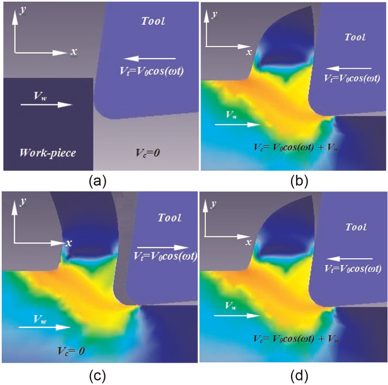
Idealized 1D vibration-assisted turning. Engagement between the tool and work-piece during one vibration cycle.

Cutting tool is driven harmonically in a linear path, which is superimposed on the motion of the workpiece. Relative to a workpiece moving at velocity V_w, the tool position and velocity are given by

$$x_t\left(t\right)=A\sin \left(\omega t\right)+V_{w}t$$

(1)

$$V_t\left(t\right)=\omega A\cos \left(\omega t\right)+V_w$$

(2)

where x_t(t) and V_t(t) are the instantaneous position and velocity at time t, A is the amplitude of the tool vibration, and ω = 2πf is the angular frequency.

In this study, cutting tool velocity model is an essential part of determining the relative cutting velocity between the vibrating tool and the workpiece, which also determines the cutting state. For a given vibration frequency f, there exists a critical workpiece velocity below which the rake face of the tool will periodically break contact with the uncut material surface. Equation (2) leads to the definition of the critical workpiece velocity V_w,crit. above which the tool rake face never separates from the uncut work surface

$$V_{w,\mathrm{crit}.}=2\pi \mathrm{fA}$$

(3)

If V < V_w,crit., then periodic interruption of cutting takes place, but if $V\ge V_{w,\mathrm{crit}.}$ , then cutting is continuous, although the relative velocity between the tool and workpiece varies harmonically. In general, interrupted cutting V < V_w,crit. is desirable as most of the benefits of UAT (extended tool life, improved surface finish, and so on) derive from the periodic separation of the tool rake face from the uncut material.

The cutting state defines the contact between the tool and the workpiece. Included in this definition are the duration of time that the tool spends cutting (t_c) and the time period for not cutting (t_s).

In the UAT, the tool and the workpiece each have a velocity component. Therefore, cutting velocity is a combination of the harmonic of the tool and the steady motion of the workpiece. This velocity combination alone provides little insight into the cutting state. Figure 2 shows a separation mode of UAT where the tool separates from the workpiece while retracting, but the workpiece catches up with the tool before the tool begins its next vibration cycle.

In Figure 2(a), the rake face has just come into contact with the uncut material and is starting to cut. In Figure 2(b), the cutting tool is machining and cutting speed is the combination of the harmonic of the tool and the steady motion of the workpiece. The duration of the first cutting cycle is t_up. In Figure 2(c), cutting tool has already withdrawn from the work. In Figure 2(d), cutting tool is shown advancing into contact with the workpiece as it commences the second cutting cycle. The duration of the full cycle is T. The portion of the cycle in which the tool is not cutting is called separation time and is designated t_s. Hence, the duration of the second cutting cycle is

$$t_2=T-t_{\mathrm{up}}-t_s$$

(4)

Therefore, in UAT process, the separation duration and cutting duration must be calculated based on the tool vibration parameters (angular velocity (ω) and vibration amplitude (A)) and the work velocity (V_w).

The workpiece motion is linear with time due to the constant work velocity. Therefore, the distance the workpiece travels while the tool is retracting would be

$$\Delta x_{\mathrm{wp}}=V_w{t}_{\mathrm{retraction}}$$

(5)

On the other hand, the tool periodically displaces from +A to −A and back to +A in the sine motion previously described. Therefore, the distance that the tool travels during its retraction would be 2A.

The probable extra distance, x_dwell, which the workpiece must travel to catch up with the tool, is

$$x_{\mathrm{dwell}}=2A-\Delta x_{\mathrm{wp}}$$

(6)

If x_dwell > 0, then the workpiece has not been caught up with the tool yet and in order to find the required time, t_dwell, the following nonlinear equation must be solved

$$x_{\mathrm{dwell}}=V_w{t}_{\mathrm{dwell}}+\underset{t_{\mathrm{up}}+t_{\mathrm{retraction}}}{\overset{t_{\mathrm{up}}+t_{\mathrm{retraction}}+t_{\mathrm{dwell}}}{\int }}\omega A\cos \left(\omega t\right)\mathrm{dt}$$

(7)

If there would be a root for this equation in the interval (0, T/4), then a second cutting cycle begins after a separation time equal to t_retraction + t_dwell and cutting continues to the end of the cycle.

On the other hand, if x_dwell < 0, then the workpiece has already been caught up with the tool, and in order to find the separation time, t_s, the following nonlinear equation must be solved

$$V_w{t}_s=\underset{t_{\mathrm{up}}}{\overset{t_{\mathrm{up}}+t_s}{\int }}\omega A\cos \left(\omega t\right)\mathrm{dt}$$

(8)

If there is root for this equation in the interval (T/4, T/2), then a second cutting cycle begins after the separation time and cutting continues to the end of the cycle.

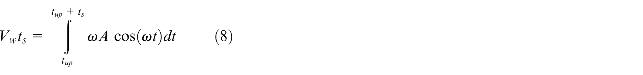
Equipped with these times, the cutting velocity (V_c) is generated by combining the work velocity (V_w) with the tool velocity (V_t) only during the cutting duration. The cutting velocity is further simplified since the tool–chip separation gives zero cutting velocity during the cycle off period (t_s). Therefore, the cutting speed is given as follows

$$\begin{array}{cc}\multicolumn{1}{c}{}& V_c\left(\tau \right)=\hfill \\ \multicolumn{1}{c}{}& \{\begin{array}{c}\hfill \begin{array}{ccc}\hfill A\omega \cos \left(\omega \tau \right)+V_w\hfill & \hfill \begin{array}{cccc}\hfill \hfill & \hfill \hfill & \hfill \hfill & \hfill \hfill \end{array}\hfill & \hfill \mathrm{nT}<\tau <\mathrm{nT}+t_{\mathrm{up}}\hfill \end{array}\hfill \\ \multicolumn{1}{c}{\begin{array}{ccc}\hfill 0\hfill & \hfill \begin{array}{ccc}\hfill \hfill & \hfill \hfill & \hfill \begin{array}{cccc}\hfill \hfill & \hfill \hfill & \hfill \hfill & \hfill \hfill \end{array}\hfill \end{array}\hfill & \hfill \mathrm{nT}+t_{\mathrm{up}}<\tau <\mathrm{nT}+t_{\mathrm{up}}+t_s\hfill \end{array}}\\ \multicolumn{1}{c}{\begin{array}{ccc}\hfill A\omega \cos \left(\omega \tau \right)+V_w\hfill & \hfill \hfill & \hfill \mathrm{nT}+t_{\mathrm{up}}+t_s<\tau <(n+1)T\hfill \end{array}}\end{array}\hfill \end{array}$$

(9)

A MATLAB program was written to calculate tool extension duration (t_up), separation duration (t_s), and cutting duration based on the tool vibration parameters and the work velocity. Equipped with these times, the cutting velocity function is generated.

The separation duration can be seen visually in terms of the work velocity and vibration parameters (Figures 3 and 4). Figure 3 shows cutting speed profiles generated for the tool vibration set to 31.25 kHz at 8 µm and work velocity of 0.5, 0.75, and 1 m/s. In this case, the separation duration is governed by the workpiece velocity and as the work velocity increases, the separation duration decreases. Figure 4 shows cutting speed profiles generated for the tool vibration set to 31.25 kHz at 1 m/s and vibration amplitude of 8, 10, and 12 µm. In this case, the separation duration is governed by vibration amplitude and as the vibration amplitude increases, the separation duration increases.

Figure 3.

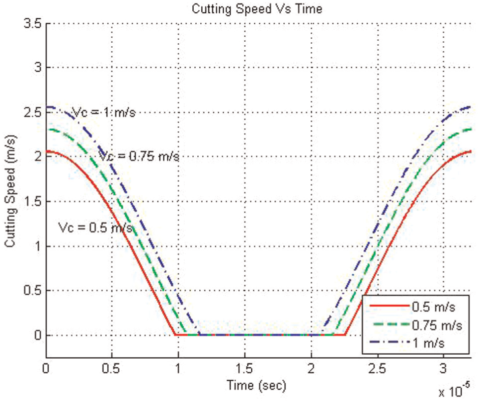
Cutting speed profiles at 31.25 kHz, 8 µm, and three different speeds: 0.5, 0.75, and 1 m/s.

Figure 4.

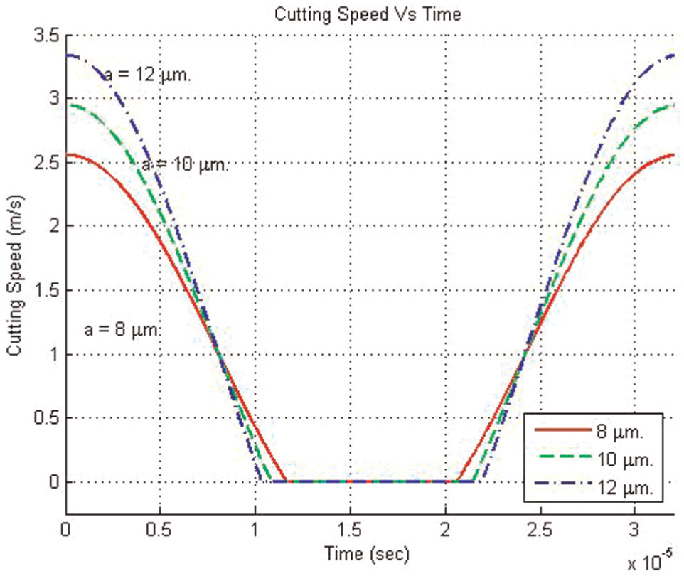
Cutting speed profiles at 31.25 kHz, 1 m/s, and three different domains: 8, 10, and 12 µm.

Modeling heat source at primary shear zone

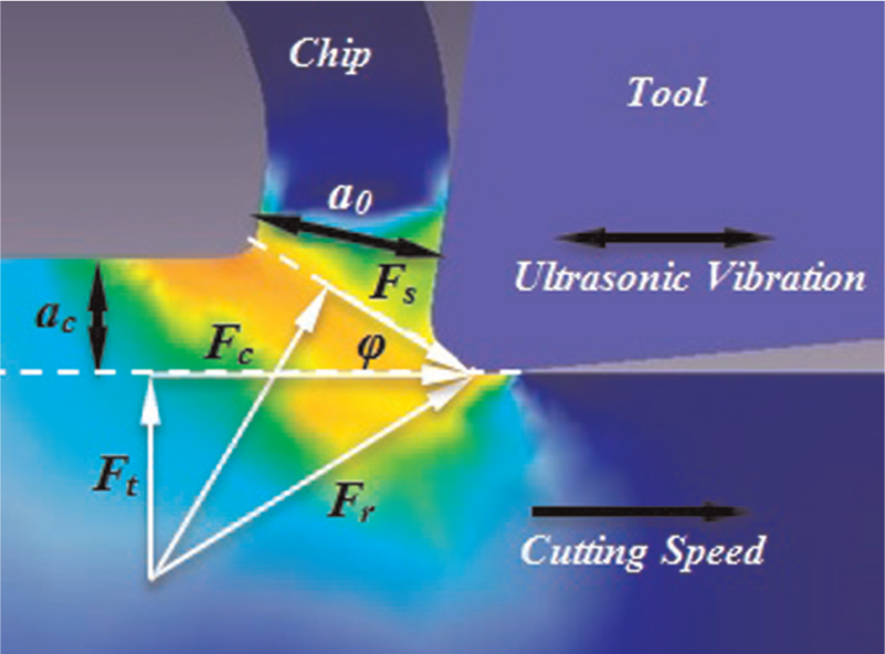
During orthogonal cutting process, heat generation occurs mainly in two principal regions: primary and secondary shear zones as shown in Figure 5(a). If cutting tool is not perfectly sharp, a third heat source would be present owing to friction between cutting tool and new workpiece surface.

Figure 5.

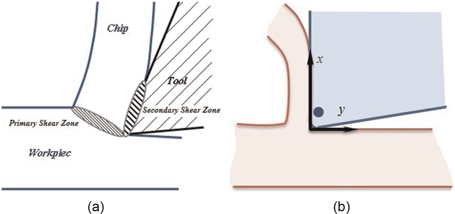
(a) Primary and secondary shear zones and (b) thermocouple position on the rake face.

Heat generated per unit depth of cut in the primary shear zone is given as follows ¹¹

$${\stackrel{·}{q}}_s=F_s{V}_s=\frac{\tau a_c{V}_c\cos \left({\alpha }_n\right)}{\cos ({\phi }_n-{\alpha }_n)\sin \left({\phi }_n\right)}\left(W\right)$$

(10)

where F_s, V_s, V_c, and a_c are shear force in shear plane, the cutting velocity component along the shear plane, the cutting velocity, and instantaneous uncut chip thickness, respectively. τ, φ_n, and α_n are the shear stress in the shear plane, shear angle, and normal rake angle, respectively. Now with heat-generated model in the primary shear zone, equation (10), average temperature on the shear plane is given as follows ¹¹

$${\overline{T}}_w=\frac{1-\chi }{\rho C}\times \frac{\tau \cos \left({\alpha }_n\right)}{\cos ({\phi }_n-{\alpha }_n)\sin \left({\phi }_n\right)}+T_0$$

(11)

where ρ, C, and T₀ are workpiece mass density, specific heat capacity, and initial temperature, respectively. χ represents the portion of the heat flux entering into the workpiece and is defined by ¹¹

$$\chi =\{\begin{array}{c}\hfill \begin{array}{ccc}\hfill 0.5-0.35{\log }_{10}(R_t·\mathrm{tg}{\phi }_n)\hfill & \hfill \hfill & \hfill 0.004\le R_t·\mathrm{tg}{\phi }_n\le 10\hfill \end{array}\hfill \\ \multicolumn{1}{c}{\begin{array}{ccc}\hfill 0.3-0.15{\log }_{10}(R_t·\mathrm{tg}{\phi }_n)\hfill & \hfill \begin{array}{ccc}\hfill \hfill & \hfill \hfill & \hfill \hfill \end{array}\hfill & \hfill R_t·\mathrm{tg}{\phi }_n\ge 10\hfill \end{array}}\end{array}$$

(12)

where $R_t=a_c{V}_c/\xi$ is thermal number and $\xi =k/\rho C$ is used to show thermal diffusivity.

In case of UAT, cutting velocity is not constant and varies periodically according to equation (9). Therefore, an effective value of cutting velocity will be used in calculation of thermal number

$$R_{t,\mathrm{uat}}=\frac{a_c{V}_{c,\mathrm{eff}}}{\xi }=\frac{a_c\underset{0}{\overset{T}{\int }}{V}_c\left(\tau \right)d\tau }{\xi T}$$

(13)

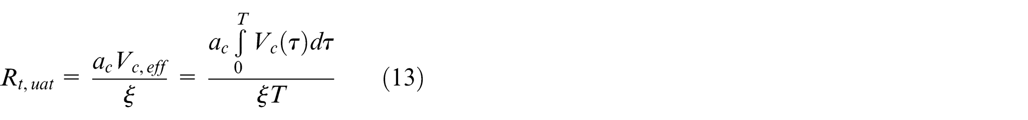
Now with thermal number calculated, equation (13), portion of the heat flux entering into the workpiece can be calculated, and as a consequence, average temperature on the shear plane during UAT can be estimated. This average temperature will be later used in section “Modeling work material during UAT” to study the effects of temperature variations on workpiece properties during UAT.

Modeling heat source at the tool–work interface

Heat generated at the tool–work interface, that is, secondary shear zone, is of major importance in relation to tool performance. ¹⁸ In this regard, tool–chip contact length is an extremely critical parameter for developing robust models in determination of this heat source.

The contact length is the distance over which a continuous chip flows over the tool rake face while maintaining contact (Figure 6). Thus, the contact length starts from the cutting edge and extends over a certain distance.

Figure 6.

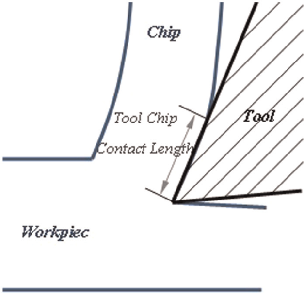
Tool–chip contact length in turning.

Up to now, many different experimental techniques have been used to measure the contact length on the rake face; the most common method used is following the traces of chip flow (or the wear traces) on the tool rake face as an indicator of the magnitude of tool–chip contact. ¹⁹ In this study, contact length is measured using the traces of chip flow (or the wear traces) on the tool rake face. Figure 7(a) shows an optical microscope image of the contact length on the rake face using a German Microscope Leitz with a magnification of 5000×. This microscope is equipped with a Canon Camera with 7 megapixel resolution. As shown in Figure 7(a), two distinct areas, with different surface texture, are recognized. The first area which starts from the cutting edge has a better surface finish and is called sticking area. The next area which is recognized by parallel traces of chip flow is called slipping contact area. The contact length obtained from the rake face tracks was also further checked by the optical microscope image of the underside tracks of the chip using chip’s metallographic cross section (Figure 7(b)).

Figure 7.

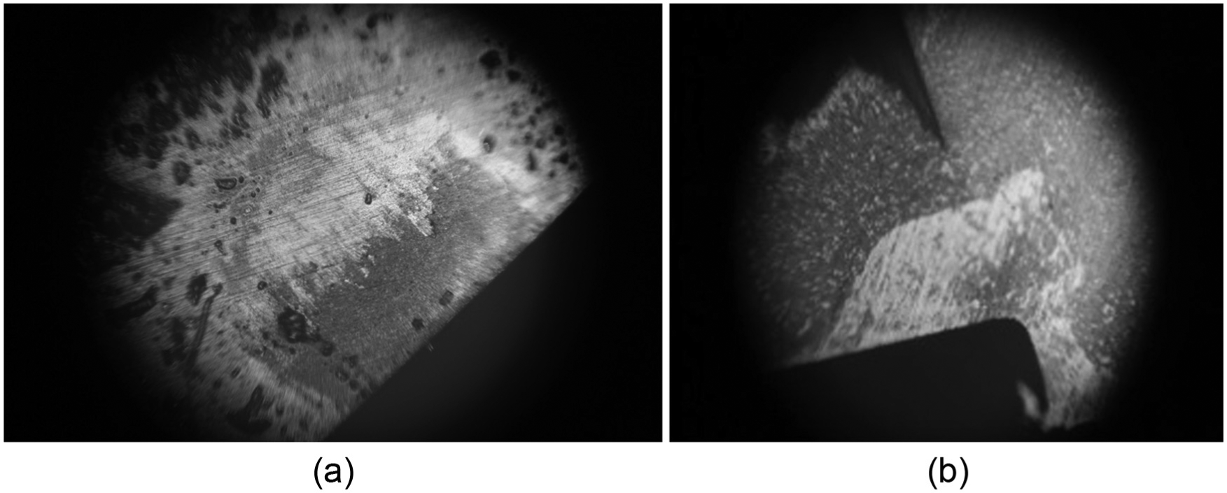
Optical microscope image of the contact length: (a) tool rake face and (b) chip metallographic.

A more realistic source flux distribution for metal cutting might be the one which has some analogy to shear stress distribution. This is because the equation that governs the stress distribution on the tool–chip contact length is of the similar form as the equation governing the shape of a heat flux distribution. Therefore, in order to discover the heat source distribution on the tool–chip contact length, all one has to do is to find the shape of shear stress distribution and then the heat source distribution at any situation is directly proportional to the shear stress at the same point.

Figure 8(a) shows a model of stress distribution as proposed by Zorev. ¹⁸ As illustrated in this figure, the shear friction stress (τ) remained constant over about the half of tool–chip contact nearest the cutting edge, sticking area (l_s), but it gradually decreased reaching 0 when the chip departed contact with the rake face, slipping area. Over the sticking area, normal stress is sufficiently high and contact area approaches the total apparent area and metal adheres to the rake face.

Figure 8.

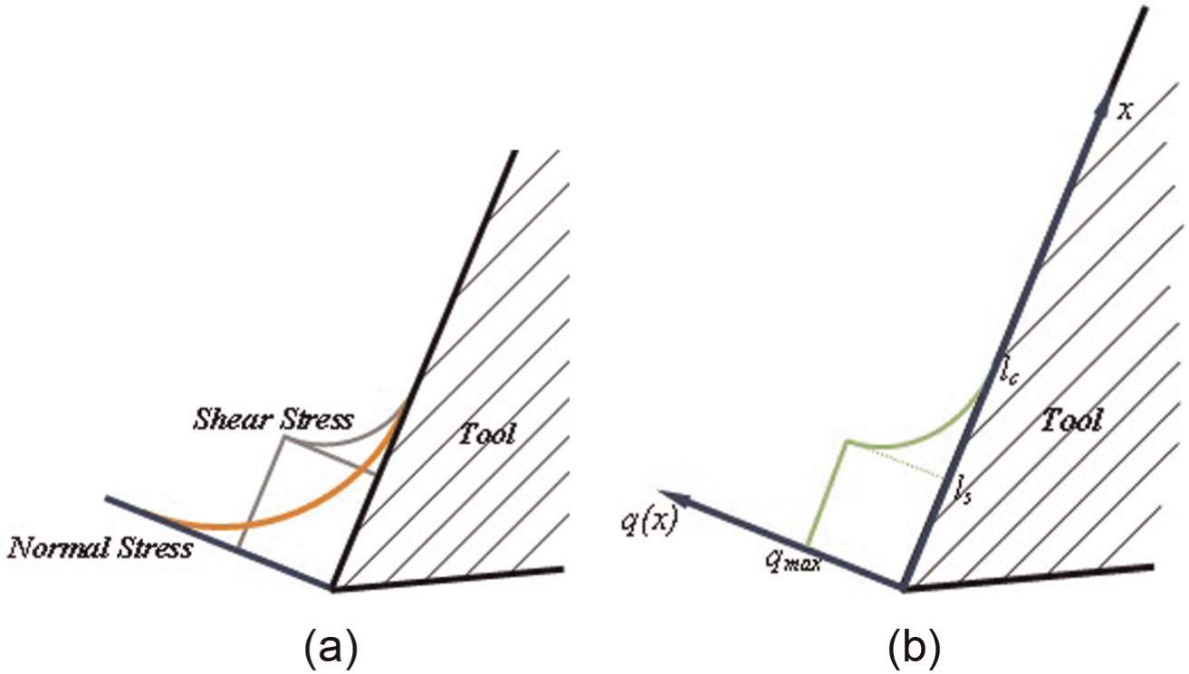
(a) Stress distribution ¹⁸ and (b) heat flux distribution on the tool–chip contact length in turning.

The same behavior would be seen from heat flux distribution function. Therefore, the heat flux function would be in the following general form

$$q_1\left(x\right)=\{\begin{array}{c}\hfill \begin{array}{ccc}\hfill q_{max}\hfill & \hfill \begin{array}{cc}\hfill \begin{array}{cc}\hfill \begin{array}{cc}\hfill \hfill & \hfill \hfill \end{array}\hfill & \hfill \hfill \end{array}\hfill & \hfill \begin{array}{ccc}\hfill \hfill & \hfill \hfill & \hfill \hfill \end{array}\hfill \end{array}\hfill & \hfill 0\le x\le l_s\hfill \end{array}\hfill \\ \multicolumn{1}{c}{\begin{array}{ccc}\hfill q_{max}\left(\frac{l_c-x}{l_c-l_s}\right)e^{\left(\frac{l_s-x}{l_c}\right)}\hfill & \hfill \hfill & \hfill l_s\le x\le l_c\hfill \end{array}}\end{array}$$

(14)

On the other hand, it is assumed that the process has orthogonal cutting geometry and the chip slides on the rake face (i.e. secondary deformation zone) with a constant average friction coefficient. Heat generated per unit depth of cut in the secondary zone is given as follows ¹¹

$${\stackrel{·}{q}}_f=F_f{V}_f=\frac{\tau a_c{V}_c\sin \left({\beta }_n\right)}{\cos ({\phi }_n+{\beta }_n-{\alpha }_n)\sin ({\phi }_n-{\alpha }_n)}\left(W\right)$$

(15)

where F_f, V_f, and β_n are the frictional force between the tool rake face and the chip contact zone, the cutting velocity component along the rake face, and normal friction angle, respectively. Dividing equation (15) by tool–chip contact length, heat flux is given as follows

$$q\left(\tau \right)=\frac{\tau a_c{V}_c\left(\tau \right)\sin \left({\beta }_n\right)}{\cos ({\phi }_n+{\beta }_n-{\alpha }_n)\sin ({\phi }_n-{\alpha }_n)l_c}\left(\frac{W}{m^2}\right)$$

(16)

Now with the cutting velocity model, equation (9), correlating the cutting time to putting heat into the tool and the separation time to letting the heat be dissipated, the definition of the heat flux equation, in UAT, is given as follows

$$\begin{array}{cc}\hfill q\left(\tau \right)=\{\begin{array}{c}\hfill \begin{array}{ccc}\hfill \frac{\tau a_c·(A\omega \cos \left(\omega \tau \right)+V_w)·\sin \left({\beta }_n\right)}{\cos ({\phi }_n+{\beta }_n-{\alpha }_n)\sin ({\phi }_n-{\alpha }_n)l_c}\hfill & \hfill \begin{array}{cccc}\hfill \hfill & \hfill \hfill & \hfill \hfill & \hfill \hfill \end{array}\hfill & \hfill \mathrm{nT}<\tau <\mathrm{nT}+t_{\mathrm{up}}\hfill \end{array}\hfill \\ \multicolumn{1}{c}{\begin{array}{ccc}\hfill 0\hfill & \hfill \begin{array}{ccc}\hfill \hfill & \hfill \hfill & \hfill \begin{array}{cccc}\hfill \hfill & \hfill \hfill & \hfill \hfill & \hfill \begin{array}{cccc}\hfill \begin{array}{ccc}\hfill \hfill & \hfill \hfill & \hfill \hfill \end{array}\hfill & \hfill \hfill & \hfill \hfill & \hfill \hfill \end{array}\hfill \end{array}\hfill \end{array}\hfill & \hfill \mathrm{nT}+t_{\mathrm{up}}<\tau <\mathrm{nT}+t_{\mathrm{up}}+t_s\hfill \end{array}}\\ \multicolumn{1}{c}{\begin{array}{ccc}\hfill \frac{\tau a_c·(A\omega \cos \left(\omega \tau \right)+V_w)·\sin \left({\beta }_n\right)}{\cos ({\phi }_n+{\beta }_n-{\alpha }_n)\sin ({\phi }_n-{\alpha }_n)l_c}\hfill & \hfill \hfill & \hfill \mathrm{nT}+t_{\mathrm{up}}+t_s<\tau <(n+1)T\hfill \end{array}}\end{array}\hfill & \hfill \left(\frac{W}{m^2}\right)\hfill \end{array}$$

(17)

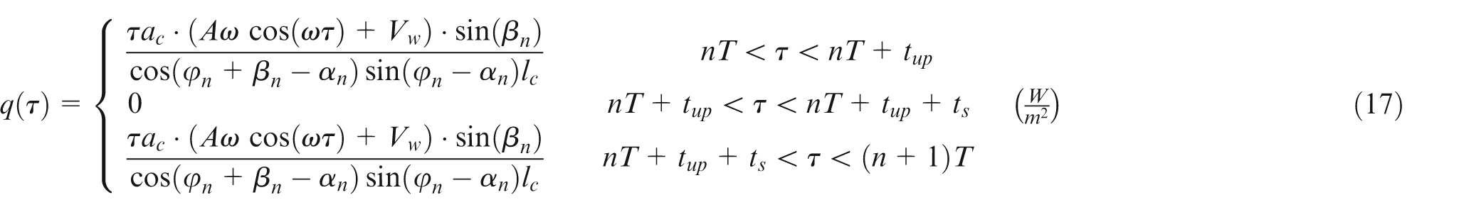
Therefore, the source heat flux of UAT process varies with time and spatial variables (x, y) and could be declared in the following general form

$$\begin{array}{c}Q\left(x,y,\tau \right)=\Gamma \left(\tau \right)q_1\left(x\right)·q\left(\tau \right)\\ \Gamma \left(\tau \right)=\frac{1}{1+\frac{k_{ch}}{k_t}\sqrt{1+Pe\left(\tau \right)}}\end{array}$$

(18)

Using chip thermal conductivity, ζ_c, and $a=0.5l_y$ , Peclet number, $\mathrm{Pe}\left(\tau \right)=V_{c}a/2{\xi }_c$ , is calculated, and therefore, the portion of the heat flux entering into the cutting tool is defined. ²⁰ Using equation (18), the effects of vibration and machining parameters on temperature distribution in UAT can be investigated.

Modeling work material during UAT

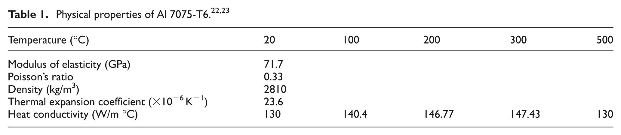
The Al 7075-T6 alloys develop the highest room-temperature tensile properties of any aluminum alloys produced from conventionally cast ingots. However, the strength of these alloys declines rapidly if they are exposed to elevated temperatures due mainly to coarsening of the fine precipitates on which the alloys depend for their strength. For instance, cutting temperature, strain, and strain rate may change the properties of the workpiece material in such conditions. Therefore, in this study, workpiece material is modeled using JC constitutive model

$$\tau =\frac{1}{\sqrt{3}}(A+B{\left(\frac{\gamma }{\sqrt{3}}\right)}^n)(1+C\ln \frac{\stackrel{·}{\gamma }}{{\stackrel{·}{\gamma }}_0})(1-{\left(\frac{T_w-T_r}{T_m-T_r}\right)}^m)$$

(19)

where τ, γ, $\stackrel{·}{\gamma }$ , and ${\stackrel{·}{\gamma }}_0$ are equivalent von Mises shear flow stress, equivalent plastic shear strain, shear strain rate, and reference shear strain rate (i.e. 1/s), respectively. T_w is temperature at primary shear zone, and all remaining parameters being material constants.

In case of orthogonal metal cutting (both CT and UAT), there exists a simple relationship between shear strain ( $\gamma$ ), rake angle ( ${\alpha }_n$ ), and shear angle ( ${\phi }_n$ ) ²¹

$$\gamma =\frac{\cos {\alpha }_n}{\sin {\phi }_n\cos ({\phi }_n-{\alpha }_n)}$$

(20)

Shear strain rate is another item of interest associated with equation (19). It may also be readily shown that in case of orthogonal metal cutting ²¹

$$\stackrel{·}{\gamma }=\frac{\cos {\alpha }_n}{\cos ({\phi }_n-{\alpha }_n)}.\frac{V_c}{t_{s.z.}}$$

(21)

where t_s.z. is the thickness of shear zone, and its reasonable mean value would appear to be about 25 µm. ²¹ Now with the cutting velocity model, equation (9), the definition of the strain rate equation, in UAT, is given as follows

$$\stackrel{·}{\gamma }\left(\tau \right)=\{\begin{array}{c}\hfill \begin{array}{ccc}\hfill \frac{\cos {\alpha }_n\times (A\omega \cos \left(\omega \tau \right)+V_w)}{\cos ({\phi }_n-{\alpha }_n)t_{s.z.}}\hfill & \hfill \begin{array}{cccc}\hfill \hfill & \hfill \hfill & \hfill \hfill & \hfill \hfill \end{array}\hfill & \hfill \mathrm{nT}<\tau <\mathrm{nT}+t_{\mathrm{up}}\hfill \end{array}\hfill \\ \multicolumn{1}{c}{\begin{array}{ccc}\hfill 0\hfill & \hfill \begin{array}{ccc}\hfill \hfill & \hfill \hfill & \hfill \begin{array}{cccc}\hfill \hfill & \hfill \hfill & \hfill \hfill & \hfill \begin{array}{ccc}\hfill \begin{array}{cc}\hfill \hfill & \hfill \hfill \end{array}\hfill & \hfill \hfill & \hfill \hfill \end{array}\hfill \end{array}\hfill \end{array}\hfill & \hfill \mathrm{nT}+t_{\mathrm{up}}<\tau <\mathrm{nT}+t_{\mathrm{up}}+t_s\hfill \end{array}}\\ \multicolumn{1}{c}{\begin{array}{ccc}\hfill \frac{\cos {\alpha }_n\times (A\omega \cos \left(\omega \tau \right)+V_w)}{\cos ({\phi }_n-{\alpha }_n)t_{s.z.}}\hfill & \hfill \hfill & \hfill \mathrm{nT}+t_{\mathrm{up}}+t_s<\tau <(n+1)T\hfill \end{array}}\end{array}$$

(22)

On the other hand, physical properties and JC constants of the workpiece material Al 7075-T6 have received considerable attention in the literature. In this work, parameters presented in Tables 1 and 2, proposed by Brar et al., ²² have been used. Knowing JC constants and equipped with equations (20) and (22), equation (19) is fully defined and all one has to do is to calculate average temperature rise on the shear plane, T_w, using equation (11).

Table 1.

Physical properties of Al 7075-T6.^22,23

Temperature (°C)	20	100	200	300	500
Modulus of elasticity (GPa)	71.7
Poisson’s ratio	0.33
Density (kg/m3)	2810
Thermal expansion coefficient (×10−6 K−1)	23.6
Heat conductivity (W/m °C)	130	140.4	146.77	147.43	130

Table 2.

Johnson–Cook constants of Al 7075-T6. ²²

Tm (°C)	n	m	C	B	A
580	0.72	1.56	0.059	674 MPa	546 MPa	Al 7075-T6

Modeling for the insert temperature field in UAT

In UAT, the heat source can be modeled as a finite plane over a semi-infinite rectangular corner (x > 0, y > 0, z > 0) (Figure 9) heated by a time-varying flux according to equation (18). This assumption would probably lead to an underestimation of temperatures in the long term but would have relatively little effect on the oscillating component of the temperature field. Therefore, if heat radiation is neglected, the governing equation and boundary condition for this problem are

$$\frac{{\partial }^2{T}_t}{\partial x^2}+\frac{{\partial }^2{T}_t}{\partial y^2}+\frac{{\partial }^2{T}_t}{\partial z^2}=\frac{1}{{\xi }_t}\frac{\partial T_t}{\partial t}$$

(23)

$$\begin{array}{cccc}\hfill -k_t\frac{\partial T_t}{\partial z}=Q(x,y,t)\hfill & \hfill z=0\hfill & \hfill 0\le x\le l_c\hfill & \hfill 0\le y\le l_y\hfill \end{array}$$

(24)

Figure 9.

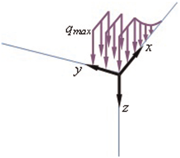
Heat source modeling as a finite plane over a semi-infinite rectangular corner.

where T_t is the temperature, k_t is the tool effective thermal conductivity, ζ_t is the effective thermal diffusivity, l_c and l_y are the dimensions of the heat source, and Q(x, y, t) is the source heat flux. All other boundary surfaces can be treated as insulated, and the initial temperature throughout the body and the temperature at infinity can be assumed to be 0.

The solution of this problem is most easily solved using Green’s functions for three mutually perpendicular instantaneous plane sources in semi-infinite half-spaces which intersect to form and eighth-space or corner. The solution due to an instantaneous heat source at time τ at the surface point x = x_p, y = y_p, z = 0 in the corner is

$$\begin{array}{cc}\multicolumn{1}{c}{}& T_G(x,y,z,x_p,y_p,0,t,\tau )=\frac{e^{-\frac{z^2}{4{\xi }_t(t-\tau )}}}{4{\left(\sqrt{\pi {\xi }_t(t-\tau )}\right)}^3}\hfill \\ \multicolumn{1}{c}{}& ·[e^{\left(\frac{-{(x+x_p)}^2}{4{\xi }_t(t-\tau )}\right)}+e^{\left(\frac{-{(x-x_p)}^2}{4{\xi }_t(t-\tau )}\right)}]·[e^{\left(\frac{-{(y+y_p)}^2}{4{\xi }_t(t-\tau )}\right)}+e^{\left(\frac{-{(y-y_p)}^2}{4{\xi }_t(t-\tau )}\right)}]\hfill \end{array}$$

(25)

Therefore, the solution for the temperature field T(x, y, z, t) in the corner can be calculated by substitution of heat flux Q(x, y, τ), equation (18), in the following equation

$$\begin{array}{cc}\multicolumn{1}{c}{}& T_t(x,y,z,t)\hfill \\ \multicolumn{1}{c}{}& =\frac{{\zeta }_t}{k_t}\underset{0}{\overset{t}{\int }}\underset{0}{\overset{l_c}{\int }}\underset{0}{\overset{l_y}{\int }}{\mathrm{T}}_{\mathrm{G}}(\mathrm{x},\mathrm{y},\mathrm{z},{\mathrm{x}}_{\mathrm{p}},{\mathrm{y}}_{\mathrm{p}},0,\mathrm{t},\tau )Q(x_p,y_p,\tau )d{y}_{p}d{x}_{p}d\tau \hfill \end{array}$$

(26)

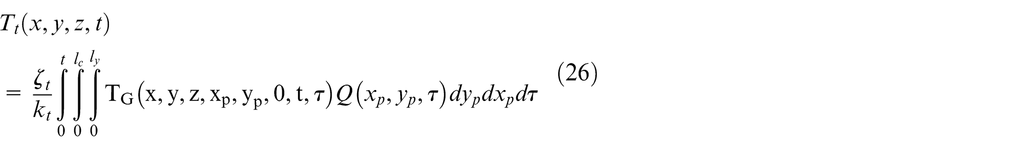
Using JC equation of workpiece and physical properties of cutting tool in combination with equation (26), the temperature distribution in cutting insert can be calculated at any point by numerically evaluating a triple integral.

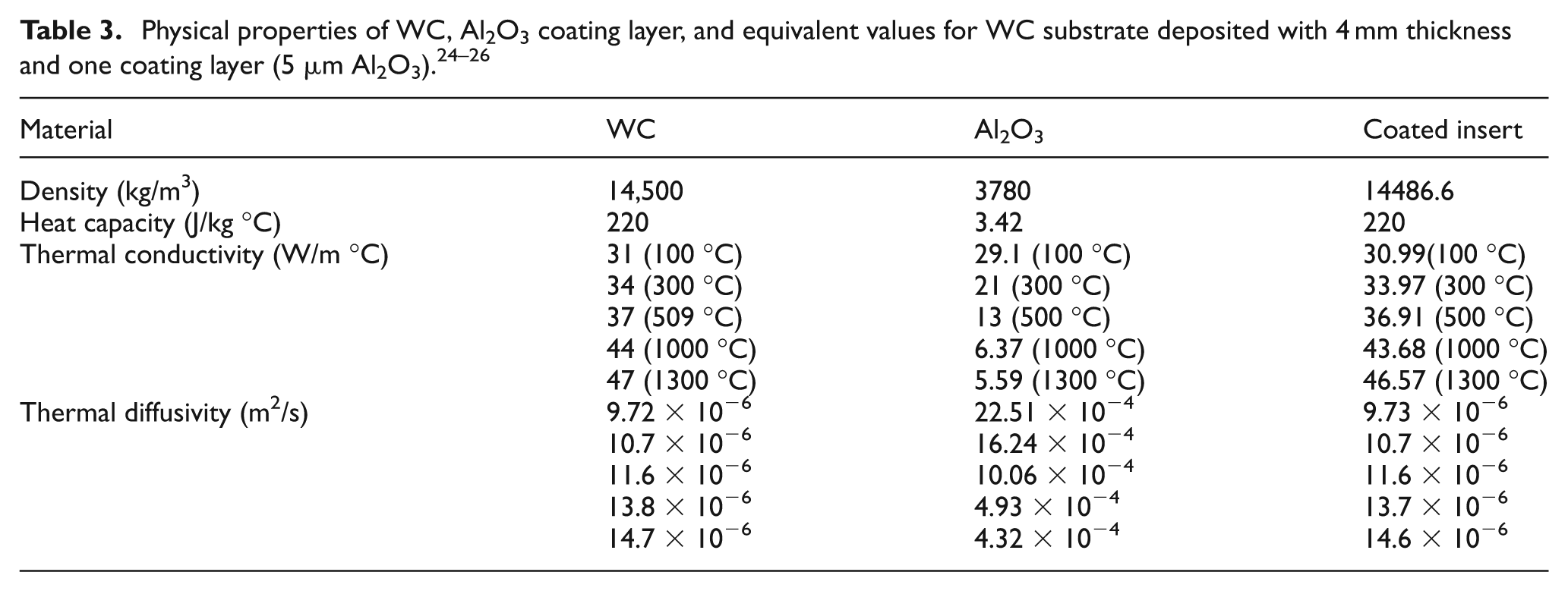
Physical properties of coating layer and WC have received considerable attention in the literature. In this work, parameters of coated layer, proposed in Ucun and Aslantas, ²⁴ and parameters of WC, proposed in Kalhori and Lundblad, ²⁵ have been used. However, in the developed mathematical model, WC turning insert with one coating layer (Al₂O₃ 5 µm) has been used. Therefore, the effective thermal conductivity and diffusivity should be calculated with respect to the number of coating layers and the thickness of each layer. This equivalent value may be expressed as follows ²⁶

$$\frac{l}{k}=\frac{l_1}{k_1}+\frac{l_2}{k_2}+\cdots +\frac{l_m}{k_m}$$

(27)

Using equation (27), one can easily calculate the effective thermal conductivity and thermal diffusivity (Table 3). On the other hand, the dimensions of the heat source (l_c and l_y) would be determined experimentally.

Table 3.

Physical properties of WC, Al₂O₃ coating layer, and equivalent values for WC substrate deposited with 4 mm thickness and one coating layer (5 µm Al₂O₃).^24–26

Material	WC	Al2O3	Coated insert
Density (kg/m3)	14,500	3780	14486.6
Heat capacity (J/kg °C)	220	3.42	220
Thermal conductivity (W/m °C)	31 (100 °C)	29.1 (100 °C)	30.99(100 °C)
	34 (300 °C)	21 (300 °C)	33.97 (300 °C)
	37 (509 °C)	13 (500 °C)	36.91 (500 °C)
	44 (1000 °C)	6.37 (1000 °C)	43.68 (1000 °C)
	47 (1300 °C)	5.59 (1300 °C)	46.57 (1300 °C)
Thermal diffusivity (m2/s)	9.72 × 10−6	22.51 × 10−4	9.73 × 10−6
	10.7 × 10−6	16.24 × 10−4	10.7 × 10−6
	11.6 × 10−6	10.06 × 10−4	11.6 × 10−6
	13.8 × 10−6	4.93 × 10−4	13.7 × 10−6
	14.7 × 10−6	4.32 × 10−4	14.6 × 10−6

The average temperature T_ave(t) over the heat source at time t

$$T_{\mathrm{ave}}(x,y,z,t)=\frac{1}{l_c.l_y}\underset{0}{\overset{l_c}{\int }}\underset{0}{\overset{l_y}{\int }}\mathrm{T}(\mathrm{x},\mathrm{y},0,\mathrm{t})\mathrm{d}\mathrm{ydx}$$

(28)

this should be the average temperature measured by the thermocouple technique on the rake face.

Experimental methodology

Orthogonal cutting tests

The experimental investigation presented here was carried out on a TB50NR lathe with a 5.5-kW spindle motor and maximum spindle speed of 2000 r/min. The workpiece used for investigation was Al 7075-T6, with chemical composition of 5.20% zinc, 2.50% magnesium, 1.6% copper, 0.23% chrome, 0.2% iron, 0.20% silicon, 0.2% manganese, 0.10% titanium, and 0.15% others. This alloy offers the highest strength of the common screw machine alloys and is heavily utilized by the aircraft and ordnance industries because of its superior strength.

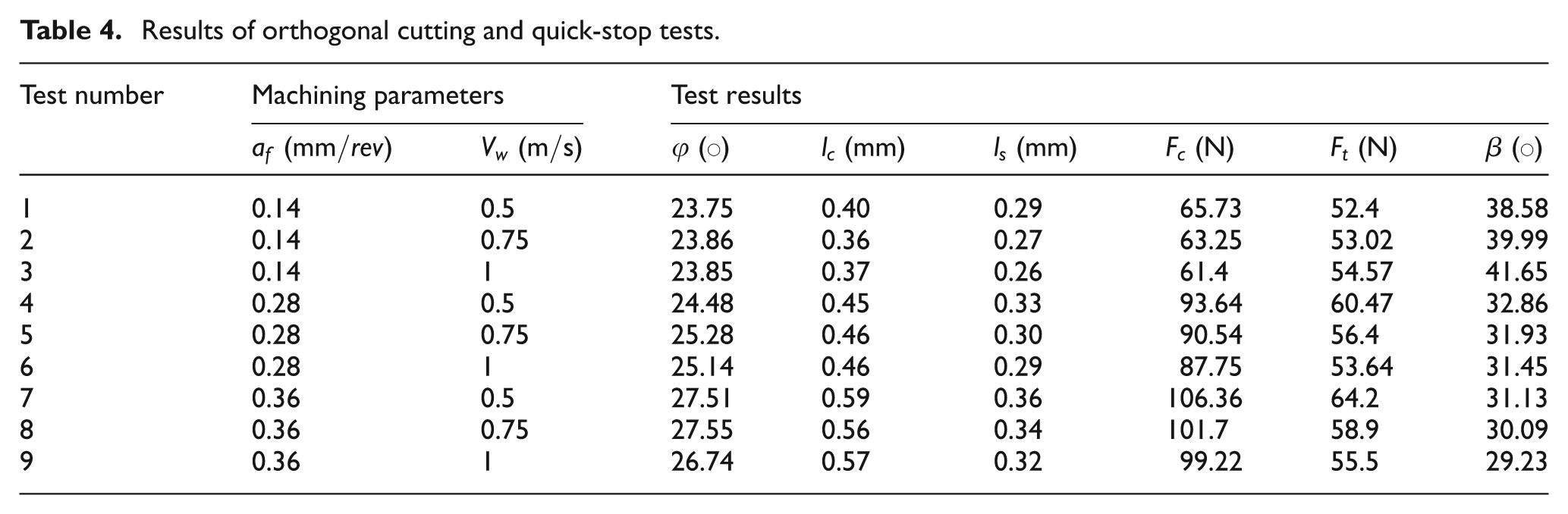
Orthogonal dry cutting of Al 7075-T6 has been performed using tungsten carbide insert with Al₂O₃ coating layer. The experiments have been conducted using tool holder with 0 rake angle, three different cutting speeds (V_w = 0.5, 0.75, 1 m/s) and three different feed rates (a_f = 0.14, 0.28, 0.36 mm/rev). In order to omit the effect of tool wear, after each test, a new insert has been used. The cutting forces were measured by KISTLER dynamometer and KISTLER 5070 charge amplifier. Calibration of the device was made before the cutting experiments by applying known weights progressively. The results of orthogonal cutting tests are presented in Table 4.

Table 4.

Results of orthogonal cutting and quick-stop tests.

Test number	Machining parameters		Test results
	$a_f(\mathrm{mm}/\mathrm{rev})$	$V_w(\mathrm{m}/\mathrm{s})$	$\phi (\circ )$	$l_c(\mathrm{mm})$	$l_s(\mathrm{mm})$	$F_c(\mathrm{N})$	$F_t(\mathrm{N})$	$\beta (\circ )$
1	0.14	0.5	23.75	0.40	0.29	65.73	52.4	38.58
2	0.14	0.75	23.86	0.36	0.27	63.25	53.02	39.99
3	0.14	1	23.85	0.37	0.26	61.4	54.57	41.65
4	0.28	0.5	24.48	0.45	0.33	93.64	60.47	32.86
5	0.28	0.75	25.28	0.46	0.30	90.54	56.4	31.93
6	0.28	1	25.14	0.46	0.29	87.75	53.64	31.45
7	0.36	0.5	27.51	0.59	0.36	106.36	64.2	31.13
8	0.36	0.75	27.55	0.56	0.34	101.7	58.9	30.09
9	0.36	1	26.74	0.57	0.32	99.22	55.5	29.23

Tool–chip contact length measurements

The measurements of chip–tool contact are very difficult and imprecise; this will affect the theoretical results. In addition to the forces, the thickness of cut chips and the contact length on the rake face were measured by means of a quick-stop device which is a modified version of the device developed by Chern. ²⁷ In the newly developed quick-stop device, the cutoff tool has been replaced with a tool holder. The aim of using new tool holder is to use cutting inserts as cutting tool which was not possible in the previous system (Figure 10).

Figure 10.

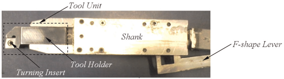
Modified quick-stop device.

During the cutting process, the quick-stop device is clamped in the lathe through the shank. As shown in Figure 10, tool unit consists of tool holder and turning insert. The cutting force is applied on the cutting insert and is resisted by a stationary block, which is constrained by the F-shaped lever.

Using the mechanism described above, the cutting tool’s edge is set to the centerline of the workpiece. Once the tool engages the workpiece, the cutting process should be continued at least for 2–3 revolutions in order to reach steady-state cutting condition. Then using F-shaped lever, tool unit is released and withdrawn suddenly during the course of cutting action. Therefore, cutting tool stops the cutting action abruptly and leaves the deformed chip attached on the workpiece. In this case, the newly formed chip does not have enough time to separate from workpiece. Figure 7(b) illustrates the cross section of such a newly formed chip in freezing mode. It is possible now to do a direct measurement from the photomicrograph of the partially formed chip. As shown in Figure 11, the section of metal in the vicinity of the partially deformed chip is ground, polished, etched, and subjected to micrographic examination.

Figure 11.

Section of metal in the vicinity of the partially deformed chip.

These experiments were also conducted on the same TB50NR lathe, and all other test conditions are the same as the force measurement tests. The experimental procedures can be described as follows: (1) preparations of workpiece and cutting inserts; (2) setting of experimental conditions; (3) cutting with Quick Stop Device (QSD), sawing and compression mounting of the chip-root samples; (4) grinding and polishing of the mounted specimen; (5) etching of the polished surface with a 5% nital (5% mixture of nitric acid in alcohol); and (6) examination of the specimen. The results of quick-stop tests are presented in Table 4.

Measurement of cutting temperature

The cutting temperature is measured by Testo 735-2 thermocouple which is embedded in the tool. The measuring device is produced by Testo Company and is equipped with Comfort software X35. Temperature setup calibration was performed before the experimental tests to ensure correct indication of cutting temperature.

The front end of the thermocouple was welded on the point where the temperature was to be measured (Figure 12). If connection between the thermocouple tip and drilled hole would not be strong enough, then the high-frequency ultrasonic vibrations will break the poor connection and thermocouple tip will slide over the drilled hole in a high-frequency motion. This high-frequency sliding motion will generate a great amount of frictional heat source, and this frictional heat source will increase thermocouple measured temperature rapidly. Therefore, in the current study, in order to omit this effect, the tip of the thermocouple was welded onto the drilled hole.

Figure 12.

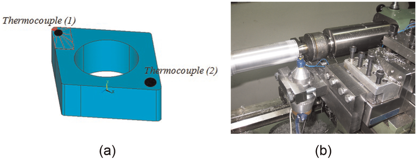
Setup of the thermocouple: (a) schematic diagram and (b) experimental setup.

In this work, in order to find the proper position for thermocouple mounting, some primary experiments were done. During this experiments, the maximum value of crater wear on the cutting tool rake face was measured using Zygo microscope. This point is probably the position in which maximum cutting temperature occurs in the cutting tool (Figure 5(b)).

Al₂O₃-coated turning inserts were used in the experiments. Two points were selected to install the thermocouples. At the selected points, a hole was drilled in the bottom of the tool with an Electro Discharge Machining (EDM) machine to embed the thermocouple. The Al₂O₃ layer acts as an insulator, and therefore, the bottom face of inserts were ground in order to remove the coating layer and let EDM process to be executed. The position of the drilled holes in all cutting inserts must be the same; otherwise, the temperature time curves in different cutting tests would not be comparable. Therefore, in the current study, special attention was given to the hole drilling process. To do so, after drilling each hole in the cutting tool, the position of the drilled holes center were controlled with a geometric position tolerance of ∅0.02 mm. This control process was done using AM-413T Dino-Lite digital microscope.[TS: Please insert appropriate symbol for ‘Ø’.]

The diameter of holes was chosen according to the probe characteristics. As a general rule, the sensing element should not be subjected to deformation. Therefore, the diameter of the drilled hole was chosen to be 0.002 greater than the thermocouple measuring tip. The diameter of the holes was 0.252 mm, and the depth of the holes was 3.9 mm.

Replacing a sensor with another one of the same type but without recalibrating may result in interchangeability error. In the current study, all measurement tests were done with the calibrated probe in which the number was 0602 0493 according to Testo catalog. This probe is ideal for measurements in small volumes and for surface measurements.

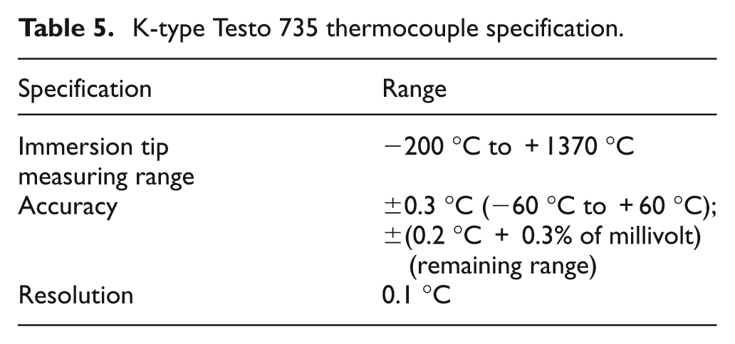
The measurement of the cutting temperature was recorded as discrete data by the Comfort software in order to further analysis. Table 5 shows the specification of K-type (NiCr-Ni) Testo 735 thermocouple used to measure the cutting temperature during the experimental tests.

Table 5.

K-type Testo 735 thermocouple specification.

Specification	Range
Immersion tip measuring range	−200 °C to +1370 °C
Accuracy	±0.3 °C (−60 °C to +60 °C); ±(0.2 °C + 0.3% of millivolt) (remaining range)
Resolution	0.1 °C

One of the most important limitations of ultrasonic-assisted machining is horn warm up due to the ultrasonic vibrations. In this research, two thermocouples have been used simultaneously in order to omit the temperature rise due to the ultrasonic vibrations (Figure 12). As shown in this figure, one of the thermocouples records temperature rise due to the combination of machining and ultrasonic vibration, and the next just records the temperature rise due to ultrasonic vibrations.

Ultrasonic equipment

In order to apply 1D vibration to the tool, a 400-W piezoelectric transducer has been employed. A 1.5-kW ultrasonic power supply transforms 50-Hz electrical supply to high-frequency (20–30 kHz) electrical impulses. These high-frequency pulses then enter the transducer and are converted to mechanical vibrations with ultrasonic frequency (31 kHz). The horn has been attached to the end of matching part of transducer by one double-ended screw, and it was made of Al 7075. Nest of the insert has a 5° relief angle, and the cutting edge is perpendicular to feed direction in order to achieve orthogonal cutting condition.

The horn has been determined by finite element analysis so that during the test, a longitudinal mode of vibration is created in the horn, and also, it creates vibration antinodes at its both ends and a vibration node at its middle. The horn was fixed from this vibration node. Figure 13 illustrates the tool fixture system and the horn displacement distribution which has been derived from modal analysis of finite element software.

Figure 13.

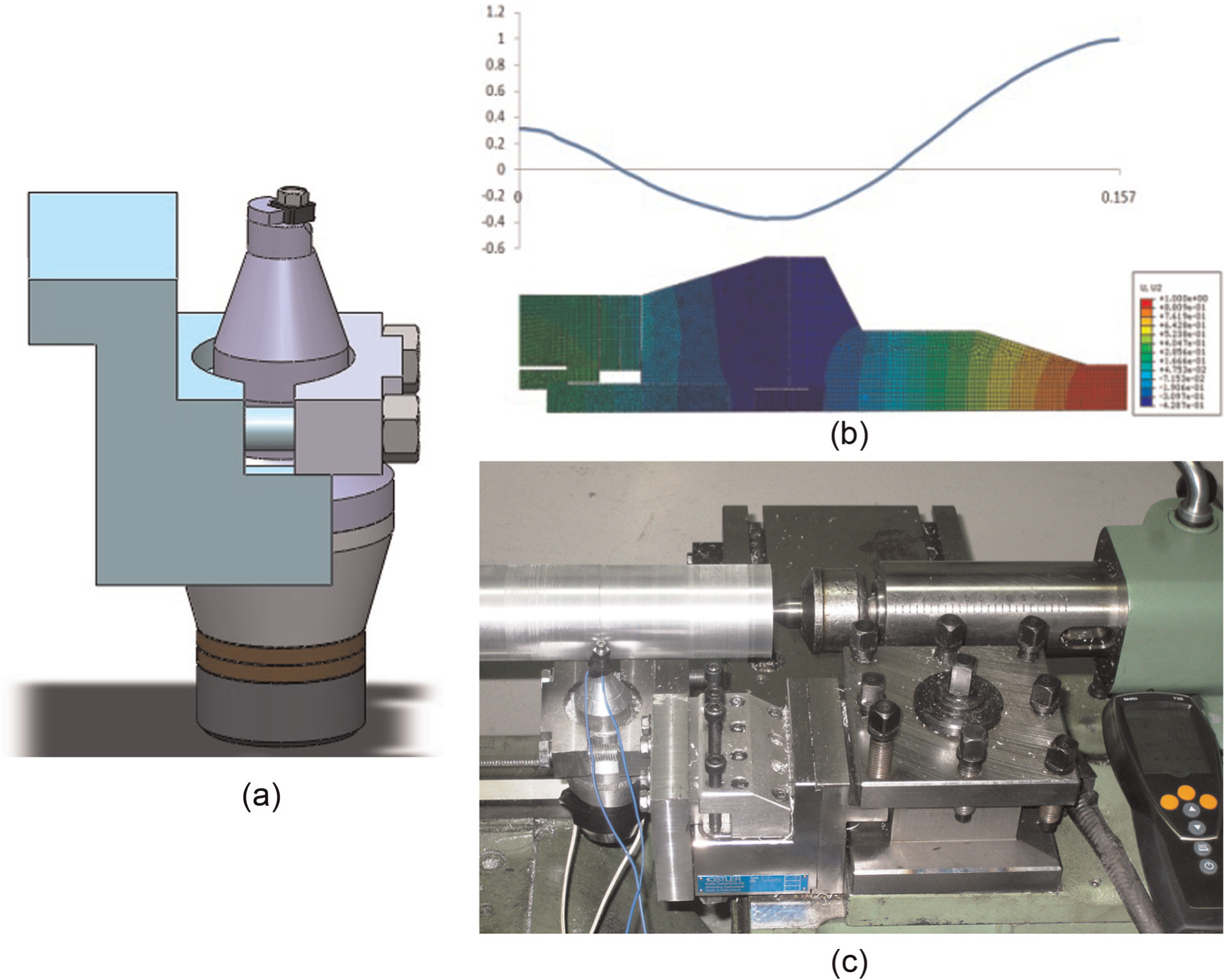
Ultrasonic equipment: (a) tool fixture and horn, (b) finite element simulation of displacement distribution, and (c) ultrasonic-assisted turning setup.

The frequency of the ultrasonic generator in each condition was tuned in a manner that the ultrasonic transducer is in its resonant frequency. The machining setup is illustrated in Figure 13(c). For measuring maximum vibration amplitude, a PU-09 gap sensor (0.4 mm/V), an AEC-5509 converter, and an oscilloscope have been used. This sensor has been located in a distance of 0.2 mm normal to the center of end face of the tool rake face, and the output in voltage can be monitored on oscilloscope. The amount of vibration amplitude changes from a maximum value to 0 and vice versa.

Experiment design and measurement

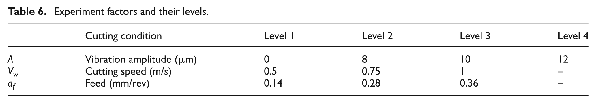
In this study, 36 sets of experiments were performed using the full factorial design of experiment method based upon two cutting parameters and the vibration amplitude. According to the recommendation of Sumitomo Company Technical Guide and several primary experiments, three levels for cutting speed and three levels for feed rate were selected. The high level of cutting speed was chosen to be less than critical speed in ultrasonic turning. The levels of the factors are presented in Table 6. A constant depth of cut of 1 mm was applied. Each test was repeated three times, and in each time, the cutting temperature and cutting force were measured.

Table 6.

Experiment factors and their levels.

	Cutting condition	Level 1	Level 2	Level 3	Level 4
A	Vibration amplitude (µm)	0	8	10	12
Vw	Cutting speed (m/s)	0.5	0.75	1	–
af	Feed (mm/rev)	0.14	0.28	0.36	–

Results and discussion

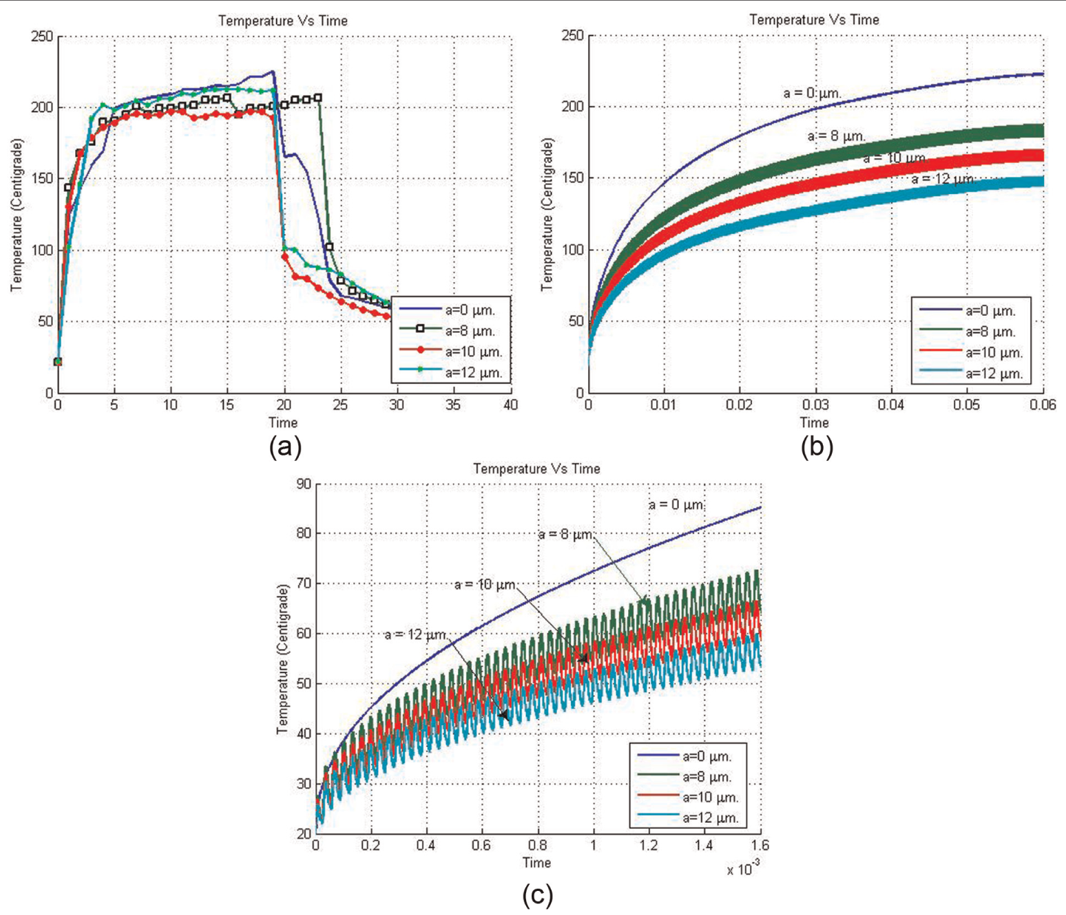
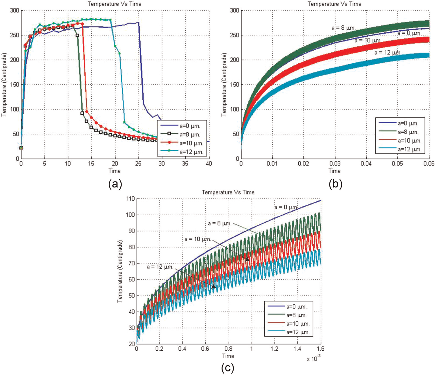
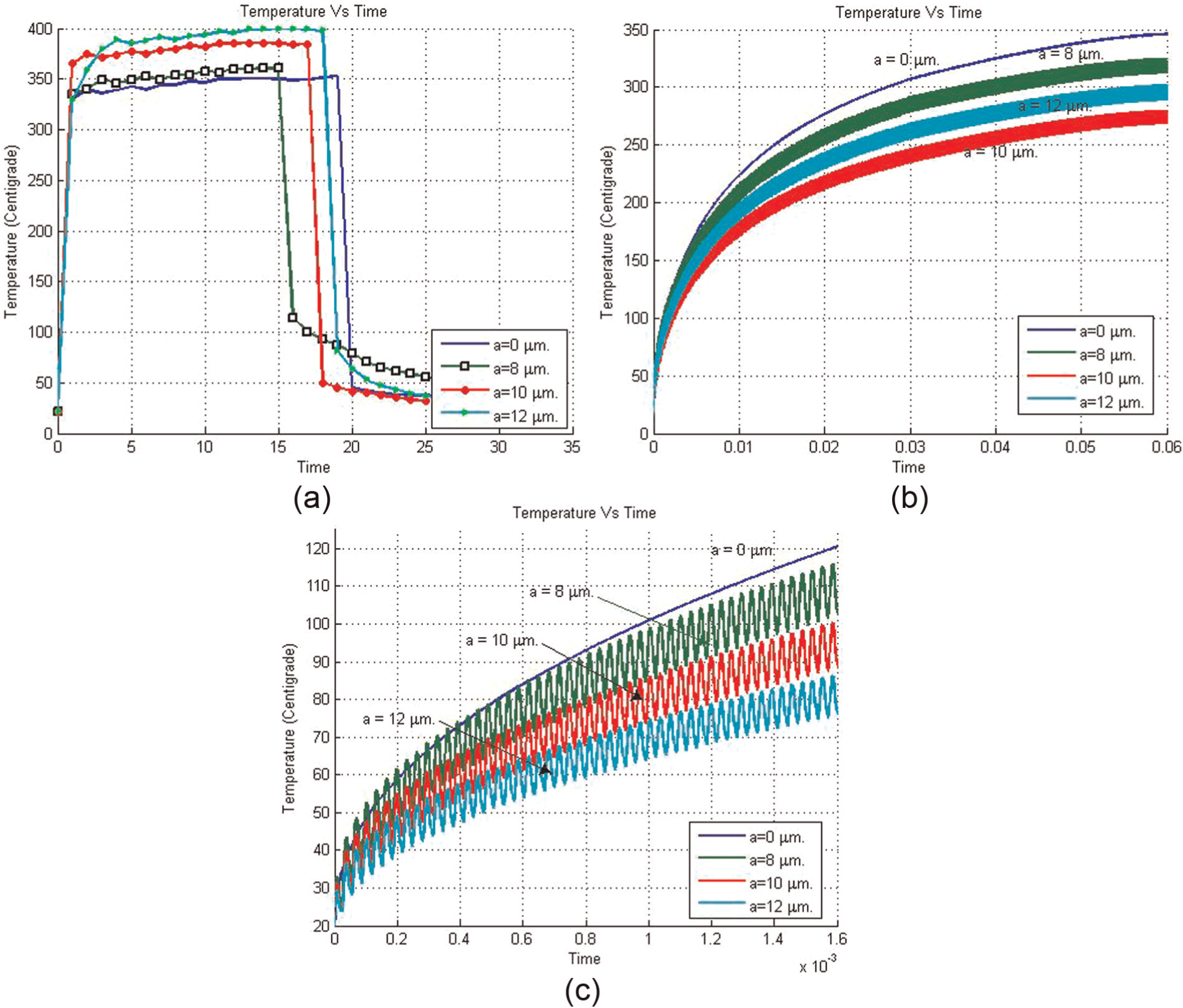
As shown in Figures 14–22, the mathematical model will reach a quasi-steady-state after 0.06 s. However, the theoretical model can be used to show the effects of cutting speed, feed rate, and vibration amplitude on the average temperature distribution during UAT.

Figure 14.

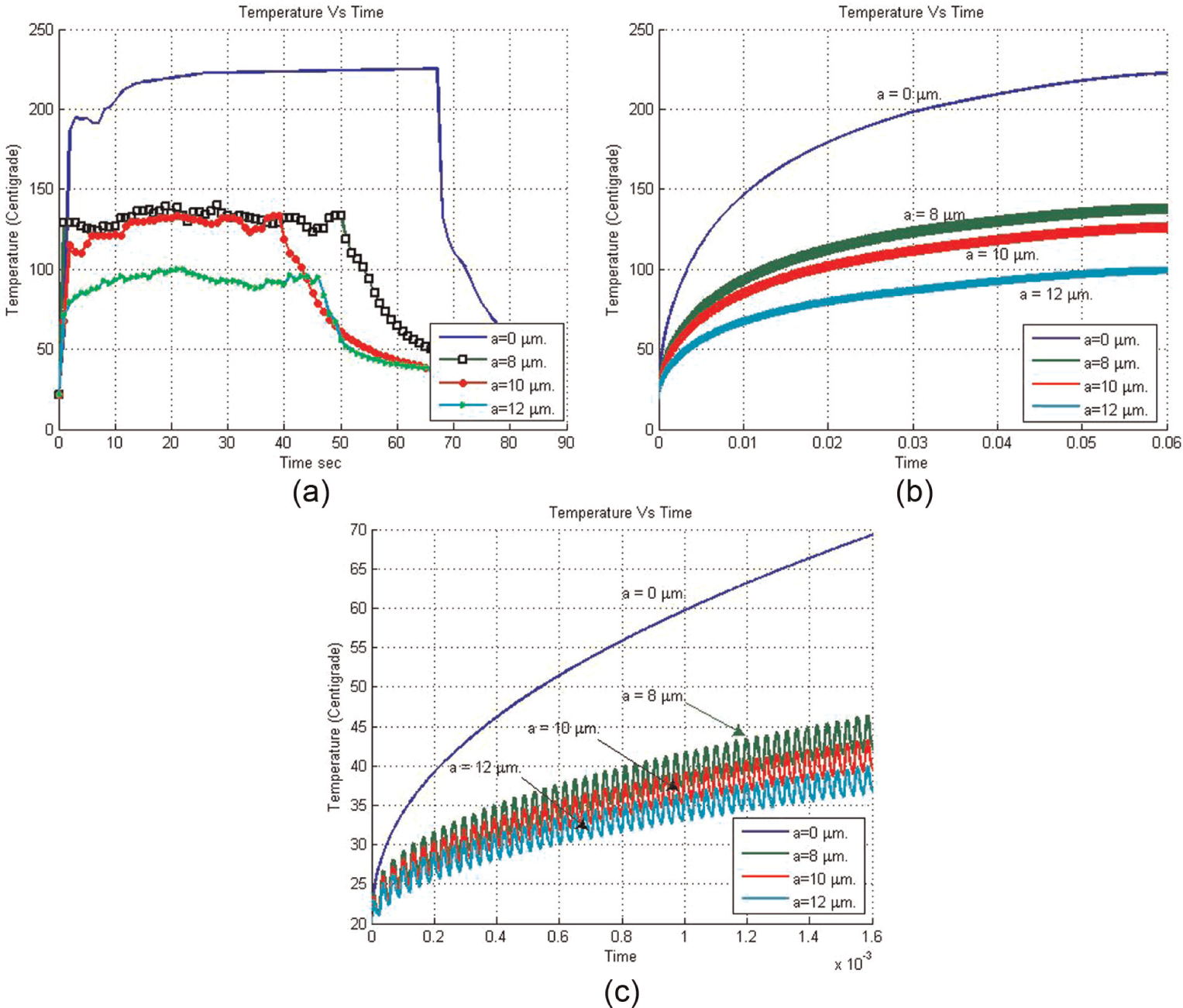
Mean temperature distribution in cutting tool: (a) experimental test, (b) mathematical model (reaching steady state), and (c) mathematical model (0, 0.0016 s) (f = 31 kHz, a_f = 0.14 mm/rev, V_w = 0.5 m/s, φ = 23.75°, β = 38.58°, x = 0.4 mm, y = 0.1 mm, z = 0.1 mm, l_c = 0.40 mm, l_s = 0.29 mm).

Figure 15.

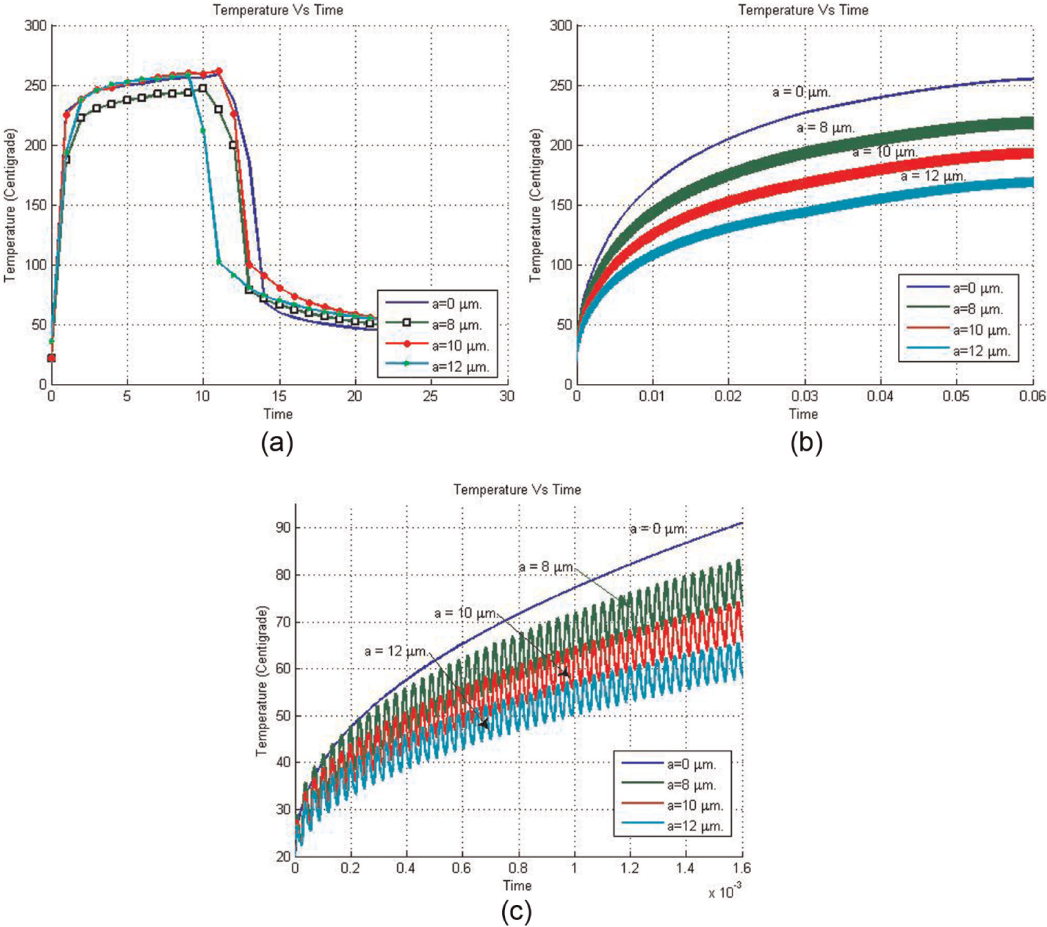
Mean temperature distribution in cutting tool: (a) experimental test, (b) mathematical model (reaching steady state), and (c) mathematical model (0, 0.0016 s) (f = 31 kHz, a_f = 0.14 mm/rev, V_w = 0.75 m/s, φ = 23.86°, β = 39.99°, x = 0.4 mm, y = 0.1 mm, z = 0.1 mm, l_c = 0.36 mm, l_s = 0.27 mm).

Figure 16.

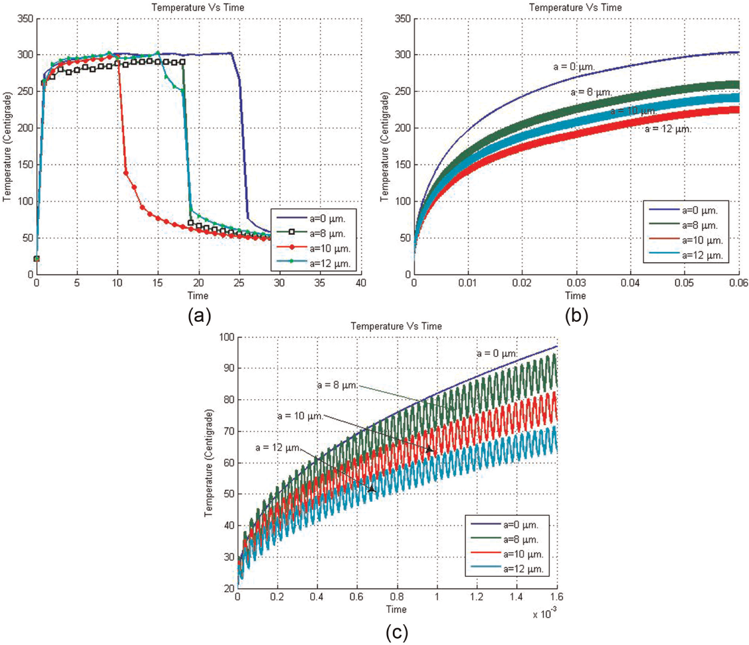
Mean temperature distribution in cutting tool: (a) experimental test, (b) mathematical model (reaching steady state), and (c) mathematical model (0, 0.0016 s) (f = 31 kHz, a_f = 0.14 mm/rev, V_w = 1 m/s, φ = 23.85°, β = 41.65°, x = 0.4 mm, y = 0.1 mm, z = 0.1 mm, l_c = 0.37 mm, l_s = 0.26 mm).

Figure 17.

Mean temperature distribution in cutting tool: (a) experimental test, (b) mathematical model (reaching steady state), and (c) mathematical model (0, 0.0016 s) (f = 31 kHz, a_f = 0.28 mm/rev, V_w = 0.5 m/s, φ = 24.48°, β = 32.86°, x = 0.6 mm, y = 0.4 mm, z = 0.1 mm, l_c = 0.45 mm, l_s = 0.33 mm).

Figure 18.

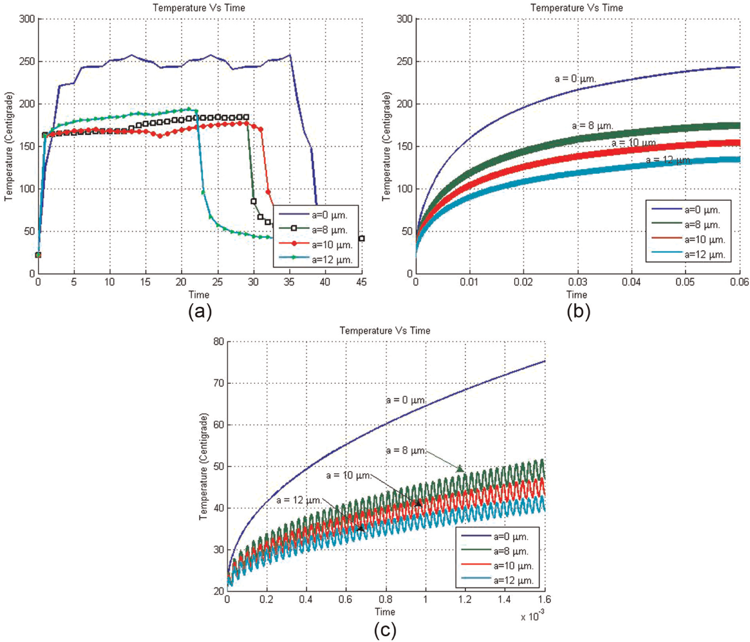
Mean temperature distribution in cutting tool: (a) experimental test, (b) mathematical model (reaching steady state), and (c) mathematical model (0, 0.0016 s) (f = 31 kHz, a_f = 0.28 mm/rev, V_w = 0.75 m/s, φ = 25.28°, β = 31.93°, x = 0.6 mm, y = 0.4 mm, z = 0.1 mm, l_c = 0.46 mm, l_s = 0.30 mm).

Figure 19.

Mean temperature distribution in cutting tool: (a) experimental test, (b) mathematical model (reaching steady state), and (c) mathematical model (0, 0.0016 s) (f = 31 kHz, a_f = 0.28 mm/rev, V_w = 1 m/s, φ = 25.14°, β = 31.45°, x = 0.6 mm, y = 0.4 mm, z = 0.1 mm, l_c = 0.46 mm, l_s = 0.29 mm).

Figure 20.

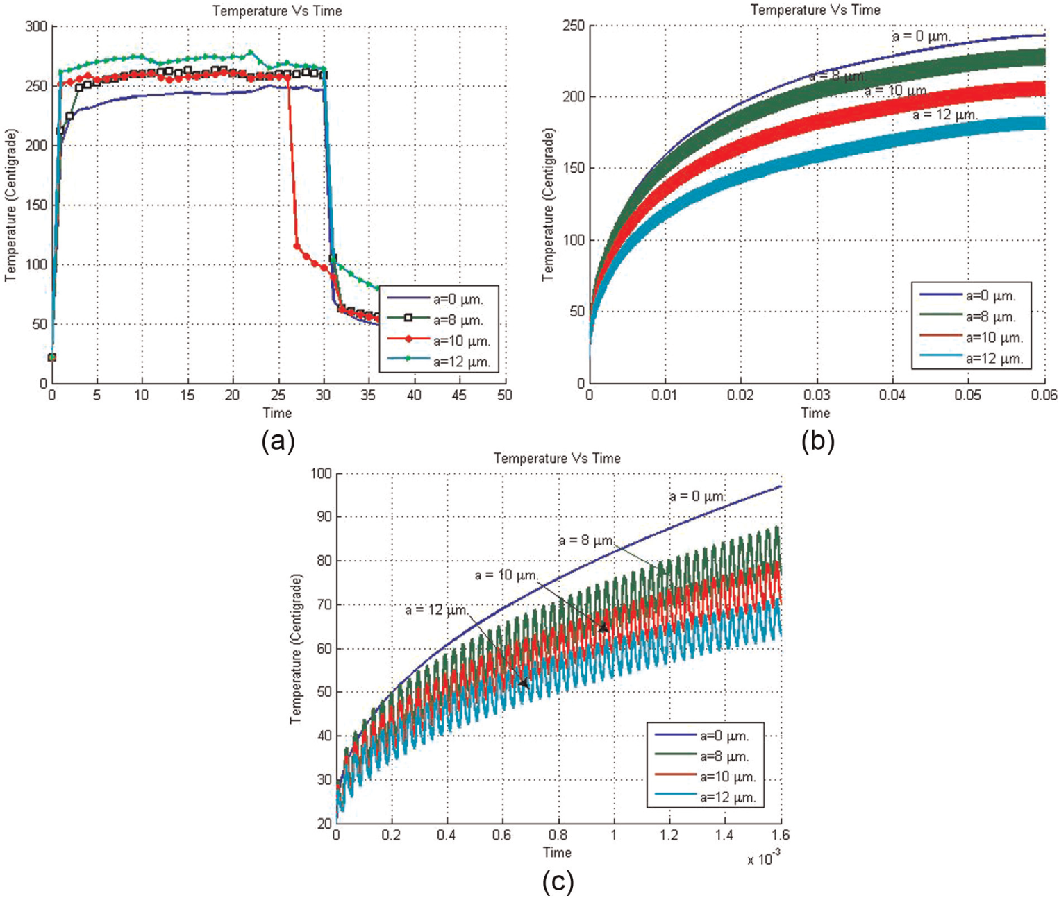
Mean temperature distribution in cutting tool: (a) experimental test, (b) mathematical model (reaching steady state), and (c) mathematical model (0, 0.0016 s) (f = 31 kHz, a_f = 0.36 mm/rev, V_w = 0.5 m/s, φ = 27.51°, β = 31.13°, x = 0.7 mm, y = 0.3 mm, z = 0.1 mm, l_c = 0.59 mm, l_s = 0.36 mm).

Figure 21.

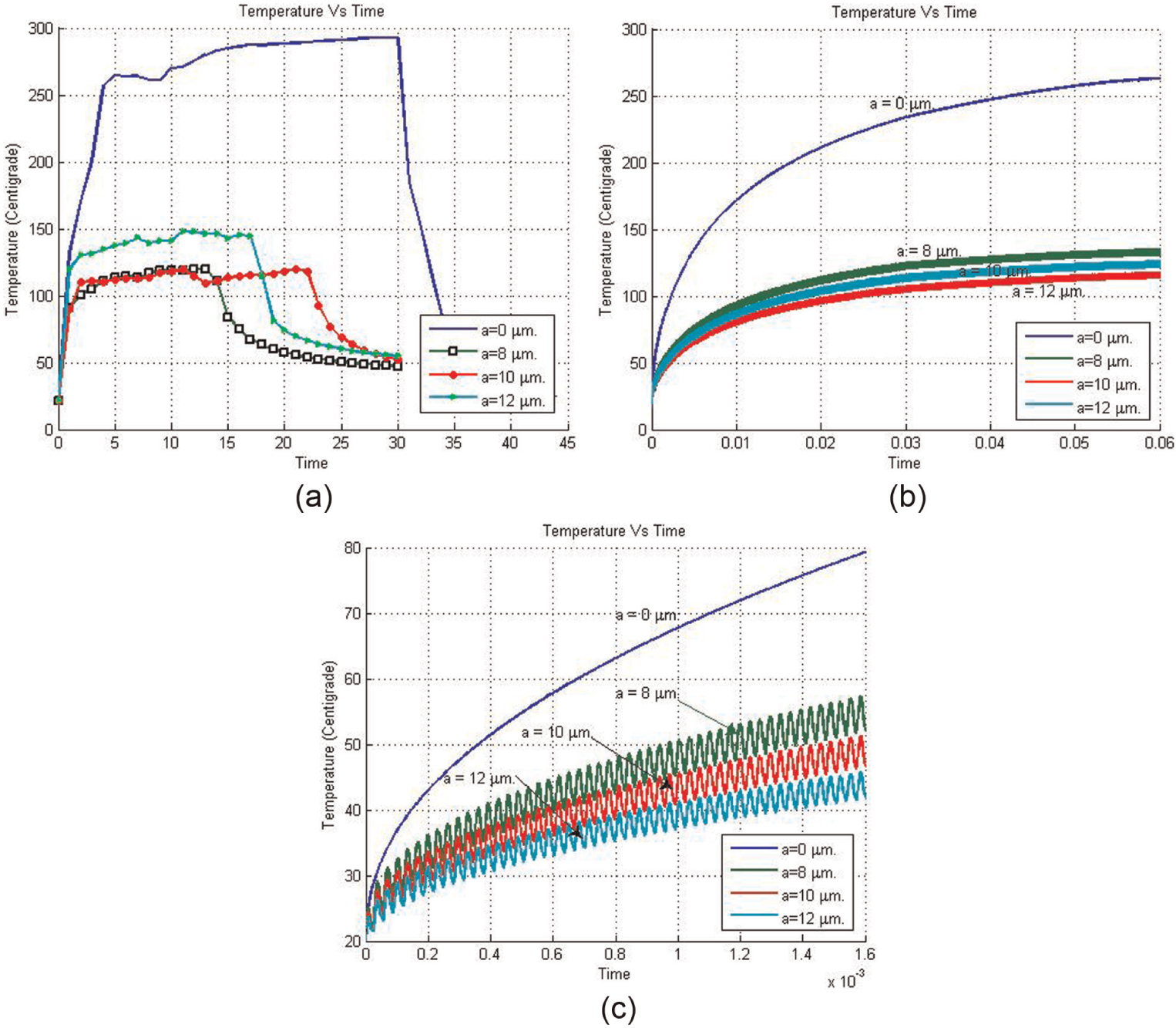
Mean temperature distribution in cutting tool: (a) experimental test, (b) mathematical model (reaching steady state), and (c) mathematical model (0, 0.0016 s) (f = 31 kHz, a_f = 0.36 mm/rev, V_w = 0.75 m/s, φ = 27.55°, β = 31.09°, x = 0.7 mm, y = 0.3 mm, z = 0.1 mm, l_c = 0.56 mm, l_s = 0.34 mm).

Figure 22.

Mean temperature distribution in cutting tool: (a) experimental test, (b) mathematical model (reaching steady state), and (c) mathematical model (0, 0.0016 s) (f = 31 kHz, a_f = 0.36 mm/rev, V_w = 1 m/s, φ = 26.74°, β = 29.23°, x = 0.7 mm, y = 0.3 mm, z = 0.1 mm, l_c = 0.57 mm, l_s = 0.32 mm).

According to the mathematical model, temperature distribution for vibration-assisted turning demonstrates an oscillation between the peak and valley temperature. At the beginning, the cutting temperature increases due to the first cutting cycle and then decreases during the separation period. The cooling effect will continue until the workpiece catches up with the tool before the tool begins its next vibration cycle. During the separation period, tool temperature will continuously decrease, but it would not reach its original thermal condition, T₀; therefore, the subsequent temperature peaks will continuously increase.

Figures 14–22 show the predicted temperature distribution for the vibration parameters set to 31 kHz at various amplitudes (8, 10, and 12 µm), feed rates of 0.14, 0.28, and 0.36 mm/rev and work velocities of 0.5, 0.75, and 1 m/s.

The experimental results show that UAT does not necessarily lower the average cutting temperature in all cases. The effectiveness of the technique is highly dependent on the value of vibration amplitude, work velocity, and feed rate. On the other hand, comparisons between the various conditions show trends with respect to each of the three varied parameters.

First, with regard to work velocity, the trend shows increasing temperatures with increasing work velocity in all cases, even for vibration-assisted turning, as deduced from the mathematical model and experimental tests. As the work velocity increases, the heat flux increases and, on the other hand, the separation duration decreases. Therefore, tool temperature will increase due to the shorter cooling cycle and much more heat flux entering the tool.

The effect of the second parameter, vibration amplitude, is very complex due to its three different effects on the process parameters: (1) as mentioned before, one of the most important limitations of ultrasonic-assisted machining is horn warm up due to the ultrasonic vibrations. Experimental measurements of tool temperature show that this warm up effect is highly dependent on vibration amplitude. In this situation, increase in vibration amplitude would increase tool’s temperature. This increase is especially considerable in the presence of high feed rates. In these cases, as shown in Figures 20–22, the process is not no more effective. Therefore, it is highly recommended to define a limiting value for vibration amplitude over which the effect of ultrasonic vibration is not no more beneficial on cutting temperature reduction. As seen in Figures 14–22, the minimum reduction in tool temperature is seen in vibration value of 12 µm, while the best results would be achieved when vibration amplitude is 8 or 10 µm; (2) increasing the vibration amplitude would increase the maximum of the tool velocity and increase the cutting temperature during the cutting cycles; and (3) increase in the tool velocity and leaving the remaining parameters constant would increase the separation time and decrease total cutting time in each cycle. Therefore, increase in amplitude vibration would improve cooling effect and the recent phenomena would decrease cutting temperature.

The trend with regard to the third varied parameter, feed rate, shows a coupling effect with vibration amplitude. At a given cutting time, increasing feed rate and vibration amplitude will decrease the effectiveness of the UAT process in lowering temperature. As feed rate increases from 0.14 to 0.36 mm/rev, UAT temperature curves get closer and closer to the CT temperature curves, and in 0.36 mm/rev, UAT curves are beyond the CT curves. It seems that this coupling effect would intensify horn’s warm up.

In the first set of experiments (Figures 14–16), feed rate is so small that the coupling effect will not take place. Therefore, tool temperature for UAT is approximately 60% of the conventional turning value and while growing with increase in feed rate and amplitude. It means that in the situations in which feed rate is so small that the coupling effect will not take place, increasing amplitude would decrease cutting temperature. This is because in small vibration amplitudes, the cooling cycle is short, and temperature reduction is not considerable.

In the second set of experiments (Figures 17–19), the coupling effect takes place and decreases the effectiveness of the process. In these cases, tool temperature for UAT is approximately 85% of the conventional turning. In the third set of experiments (Figures 20–22), the coupling effect is dominant and the process is no more effective.

Conclusion

The main goal of this article is to study the average tool temperatures in UAT of aerospace aluminum using Al₂O₃-coated tools. To achieve this objective, a mathematical model is developed, and the results are compared with experimental measurements of the average cutting temperature from UAT tests. According to the achieved results, it can be concluded that

1. Experimental temperatures attain steady state, but the mathematical model will reach a quasi-steady-state. However, the theoretical model can be used to show the effects of cutting speed, feed rate, and vibration amplitude on the average temperature distribution during UAT.

2. Increasing work velocity would increase tool temperature in all cases, even for vibration-assisted turning, as deduced from the mathematical model and experimental tests.

3. UAT does not necessarily lower the cutting temperature in all cases, and the effectiveness of the technique is highly dependent on the value of vibration amplitude, work velocity, and feed rate.

4. At a given cutting time, high feed rate and vibration amplitude will decrease the effectiveness of the UAT process in lowering temperature. In the situations in which feed rate is so small that the coupling effect will not take place, increasing amplitude would decrease cutting temperature.