A new model for contact geometry in single-point incremental forming

Abstract

Because the deformation within single-point incremental forming occurs in a small region around the area of contact, understanding the size and shape of the contact patch is useful to model process conditions. The following presents a new model of contact geometry, wherein contact geometry is derived from the intersection of the tool with the regions that have already been formed. Because this method allows for contact geometry to be determined based on measurable surrounding features, experimental measurements of contact geometry are performed to quantify the contributions of tool diameter, step size and wall angle on contact area.

Introduction

Single-point incremental forming (SPIF) is a sheet metal forming technique that uses a small, generic tool to form parts from sheet metal. Because a single tool can be used for a wide variety of shapes, SPIF is ideally suited as a custom manufacturing or prototyping method. A review of the configuration of SPIF and applications was published by Jeswiet et al. ¹ in 2005.

Because the majority of deformation in SPIF occurs in a small region around the tool, it is useful to understand the size and shape of this contact area. Contact geometry is useful for modelling aspects such as contact force distributions, ² material distribution and failure prediction ³ and tribological conditions. While the actual area of contact is not directly needed for these purposes, it is nonetheless useful to have an understanding of the geometry of the contact patch and the influence from parameters such as tool diameter, stepdown and wall angle. Recently, electric current has been used to forming limits in SPIF,^4–6 a process that can benefit greatly from the ability to quantify current density. By knowing the contact area, the current density can be determined. It is therefore proposed that a general model of contact area is useful for a wide variety of applications with SPIF, particularly one that allows for direct measurements to be taken.

In the following, a model is presented to describe the shape and size of the contact geometry. The shape of this contact region can be seen in Figure 1 as the smear mark left by a tool at the bottom of a formed part. This model expands on previous models by accounting for tool diameter, step size and wall angle. This model is also developed using geometry that can be directly measured, allowing for experimental evidence to be incorporated into contact models.

Figure 1.

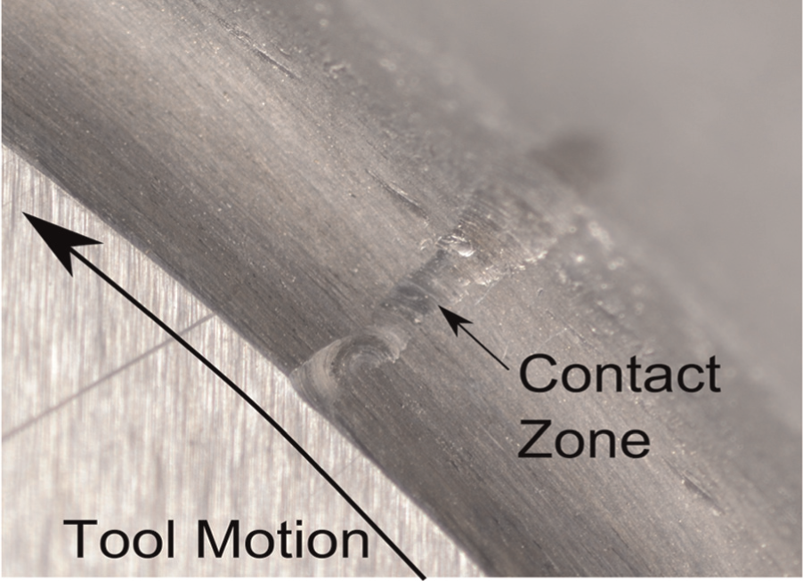
Smear mark left by the tool indicating the shape of the contact geometry.

Background

Direct measurement of the contact shape is made difficult by the non-planar shape and complex boundaries. Furthermore, the actual contact area during forming is obstructed by the tool during forming. Because quantitative measurements have not been made, our understanding of the contact region has so far been based on a variety of models that have been proposed over the years.

One of the simplest models used is the ideal contact zone, presented by Szekeres ⁷ in 2003 (left image in Figure 2). This model was used to determine the mean contact angle between the tool and the sheet for the purposes of force measurement. The actual marks left by tools, however, show that there is contact inside of the toolpath as well, and an expanded model was proposed by Hamilton ⁸ to include indentation of the tool into the sheet, the shape of which is shown on the right in Figure 2.

Figure 2.

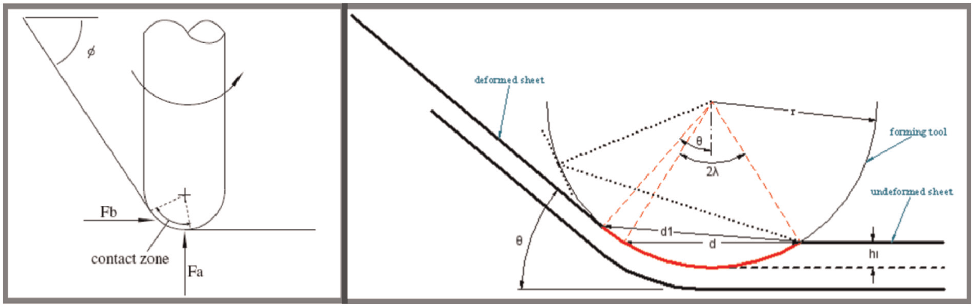
Contact models developed by Szekeres (left) and Hamilton (right).

A similar model for indentation that accounts for tool wrap on the inside of the toolpath was proposed by Aerens et al. ² and used to relate the radial and axial force components in the tool. This model used three angles α, β and γ to represent the angle of contact due to wall angle, scallop angle due to the previous toolpath and the additional angle due to indentation into the sheet. The angle of wrap around the inside of the tool, γ, is given by equation (1)

$$\gamma =17.2{\left(\frac{d_t}{10}\right)}^{-c}$$

(1)

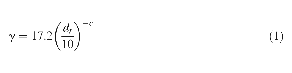
where c = 2.54 for aluminium alloys and c = 1.20 for AISI 304. This method was used with some success to represent the relation between radial and axial force on the tool due to wrap around the tool. Both Hamilton’s and Aerens’ models present the contact area as a ribbon of constant thickness in the direction of tool travel. Silva et al. ⁹ modelled the contact area as a spherical section representing the tool, intersecting the previous toolpath. This method produced a predicted shape that agrees reasonably well with observed smear marks left by the tool; however, no method of quantifying this shape was presented.

Finite element simulations were performed by Eyckens et al. ¹⁰ to estimate the contact forces at the forming zone. The stress plots presented appear to most closely reflect the curved shape of the smear marks in Figure 1. Mirnia and Dariani ¹¹ used the numerical upper bound approach to determine the regions of the sheet in contact with the tool, which was then used to predict tangential forces. There were no experimental results directly quantifying contact area as there is no current method to experimentally measure contact area.

Modelling contact area

As the tool moves along its forming pass, a cylindrical trough is left behind the tool from where the material has been formed into shape. During fully established forming, a trough is also present in front of the tool, left from the previous forming pass. Because the tool cannot be in contact with the sheet inside these troughs, a cylindrical section of trough radius may be removed from the tool hemisphere, leaving a ribbon-shaped section of the hemisphere where it contacts the sheet as shown in Figure 3. The area of the tool that remains after removing sections that are not in contact with the sheet is therefore the contact patch.

Figure 3.

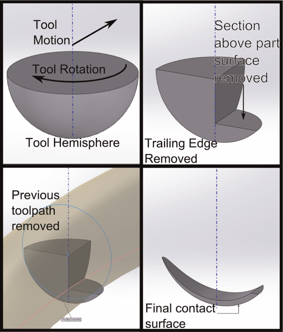
Development of the contact area by removing regions that are not in contact with a tool hemisphere.

Using this method, the effects of wall angle, scallop due to stepdown as well as springback effects can be accounted for by varying the position and diameter of the troughs, as well as the height above the tool bottom of bottom of the part. By using a curved trough intersecting the tool, part curvature can also be accounted for; however, to improve measurement accuracy in this study, part walls are kept straight. The contact area can then be determined by knowing the following:

• Location and diameter of the tool,

• Z-depth of the bottom plane of the part,

• Location and diameter of the trough left by the previous toolpath.

Numerical derivation

The contact area is calculated by integrating the perimeter of the tool at angle ψ from the tool axis, while subtracting the regions not in contact with the sheet. At a given angle ψ, the tool projects a circle of radius s in the plane of the sheet, as shown in Figure 4. The coordinates R, T and Z are defined here as the direction to the outer wall, the direction of tool travel and the tool axis, respectively.

Figure 4.

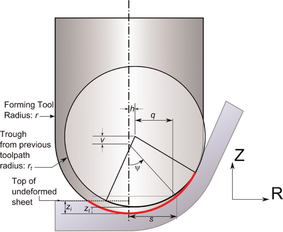
Contact geometry in the R-Z plane. The circular section in the middle represents the trough left by the previous forming pass.

The tool is intersected by a cylindrical shape, representing the previous toolpath, in the R-Z plane of radius r_trough and offset from the tool centre by h horizontally and v vertically.

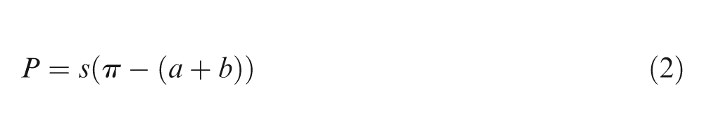
For a given angle ψ, the trough projects a straight-walled cut through the tool in the R-T plane, producing a rectangular projection of width 2q which can be seen in Figure 5. The perimeter P of the tool intersection for a given angle ψ is therefore calculated using equation (2)

$$P=s(\pi -(a+b))$$

(2)

Figure 5.

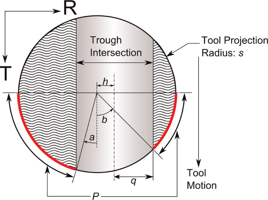
Contact patch viewed from the top.

The angles a and b represent the angle from the path of the tool to either edge of the trough where it intersects the periphery of the tool. For the section of the tool below the bottom of the trough, a and b are both equal to 0. The angles a and b are given by equation (3)

$$a={\sin }^{-1}\left(\frac{q-h}{s}\right)b={\sin }^{-1}\left(\frac{q+h}{s}\right)$$

(3)

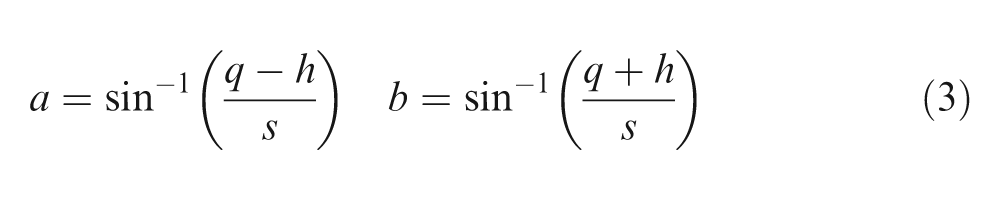
The angles a and b are a function of the width q of the trough at a given angle ψ as well as the horizontal distance h between the centre of the tool to the centre of the trough. The instantaneous radius q of the intersecting trough is calculated using equation (4)

$$q=\sqrt{r_{\mathrm{trough}}^2-{(r_{\mathrm{trough}}-(r_{\mathrm{trough}}-r\cos \psi +z_t))}^2}$$

(4)

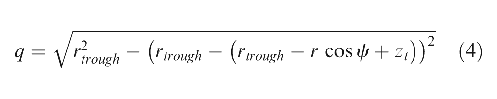
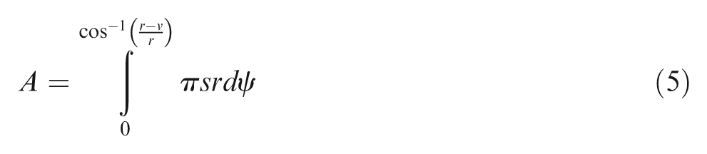
In the above equation, z_t, shown in Figure 4, is the height of the bottom of the trough above the bottom of the tool. Area is determined in three discrete steps: below the trough, above the trough but below the plane of the top of the sheet and above the sheet. Below the bottom of the trough the area is calculated by the following integral

$$A=\underset{0}{\overset{{\cos }^{-1}\left(\frac{r-v}{r}\right)}{\int }}\pi \mathrm{srd}\psi$$

(5)

Above the bottom of the trough, the area is calculated as

$$A=\underset{{\cos }^{-1}\left(\frac{r-v}{r}\right)}{\overset{{\cos }^{-1}\left(\frac{r-z_i}{r}\right)}{\int }}(\pi -(a+b))\mathrm{srd}\psi$$

(6)

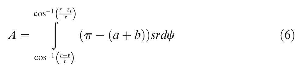
Finally, above the plane of the sheet bottom, only the side nearest the wall is in contact. This is accounted by reducing the angle to which the instantaneous radius is swept from 180° to 90°, thereby only considering one side of the trough. The final stage of the area integral is

$$A=\underset{{\cos }^{-1}\left(\frac{r-z_i}{r}\right)}{\overset{\pi /2}{\int }}(\frac{\pi }{2}-b)\mathrm{srd}\psi$$

(7)

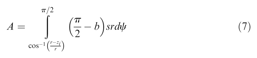
It should be noted that while the upper limit to this integral is listed as ψ = π/2, the area added by a section will become 0 prior to that when b = π/2. This represents the point at which the wall no longer contacts the tool.

Experimental method

To determine the contributions of wall angle, tool diameter and stepdown on contact area, a series of experiments were performed, measuring the contact area for each sample. Using the method above, contact patch areas can be determined from experimental data by measuring the trough radius r_trough, horizontal and vertical distance from tool to trough h and v, respectively, and the depth of indentation z_I. Given a known tool position and radius, these values can be determined by measuring the trough radius and position, and the depth of the sheet bottom relative to the tool, as shown in Figure 6.

Figure 6.

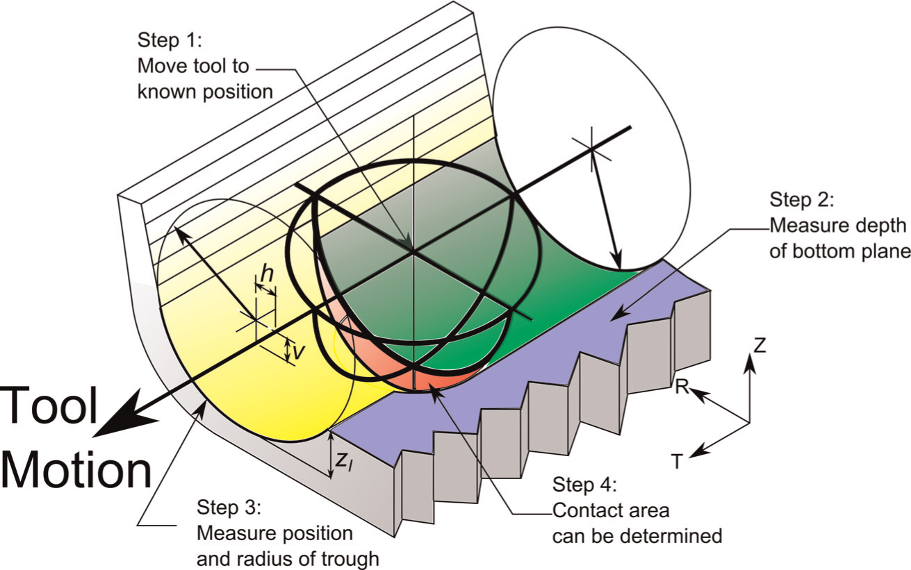
Experimental measurement method to find contact area.

Measurements were taken by forming a square pyramidal frustum, then measuring the size and position of the trough ahead of the tool as well as position of the sheet bottom to establish the indentation depth. Measurements were taken with the tool in place, in a known position, allowing recorded measurements to be stated as relative positions to the tool centre.

The features in Figure 6 were then measured by recording the positions of points using a coordinate measuring machine (CMM) fitted with a point probe. Between tests, the probe tip was re-ground and calibrated against a spherical calibration target. Features such as circles and planes were then constructed from the measured data using commercial CMM software. Measurements of the blankholder were also taken to allow the measurements to be aligned with the fixture coordinate system.

A 2³ factorial experimental design was implemented with an additional six centrepoint runs, varying the tool diameter, wall angle and stepdown size as shown in Figure 7. Measurements were taken with the tool in place to ensure that the conditions during measurement are as close as possible to those during forming.

Figure 7.

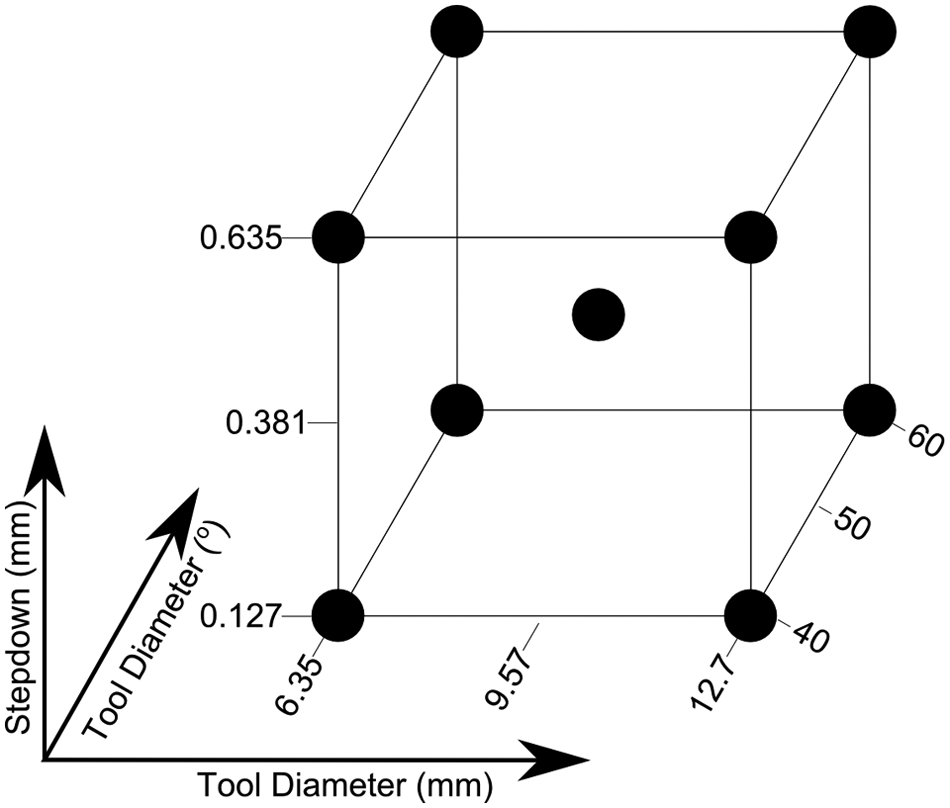
Experimental design.

To establish the z-position of values accurately, tools are first machined in the mill spindle against a turning tool fixed to the forming rig. A flat-ended reference object is then machined against the same turning tool. The reference tool is then moved to a known distance above the tool compensation plane, allowing measurement of the tool compensation plane and therefore the z-position of the tool.

Tests were performed in random order. Tool diameter was varied as 6.35, 9.57 or 12.7 mm, as these are within the range of most commonly seen tool diameters. Stepdown was varied between 0.127, 0.381 and 0.635 mm. Finally, wall angle was varied between 40°, 50° and 60°. Tests were performed on AA 3003-O with an initial thickness of 1.57 mm. Sheet material and thickness were kept constant in order to reduce the samples required while having greater sample accuracy.

Results

Total area

The area was calculated from the measured geometry using the methods described above. The final calculated contact area for each test is summarised in Figure 8. The fitted surfaces in Figure 8 are used to show general trends, as it is more useful to model each of the individual contributing factors v, h, r_t and z_I. The plane shown in Figure 8 is shown as a slice through the midpoint at the third factor, while points at the corners represent experimental runs that have a varied third factor.

Figure 8.

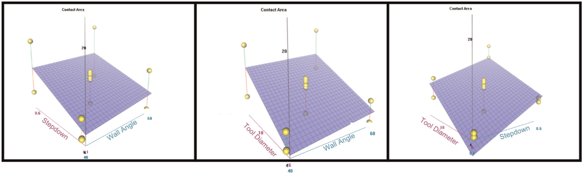
Total contact area as a function of the factors tool diameter, wall angle and stepdown. Each surface is a slice with the third factor set to the midpoint.

Indentation depth

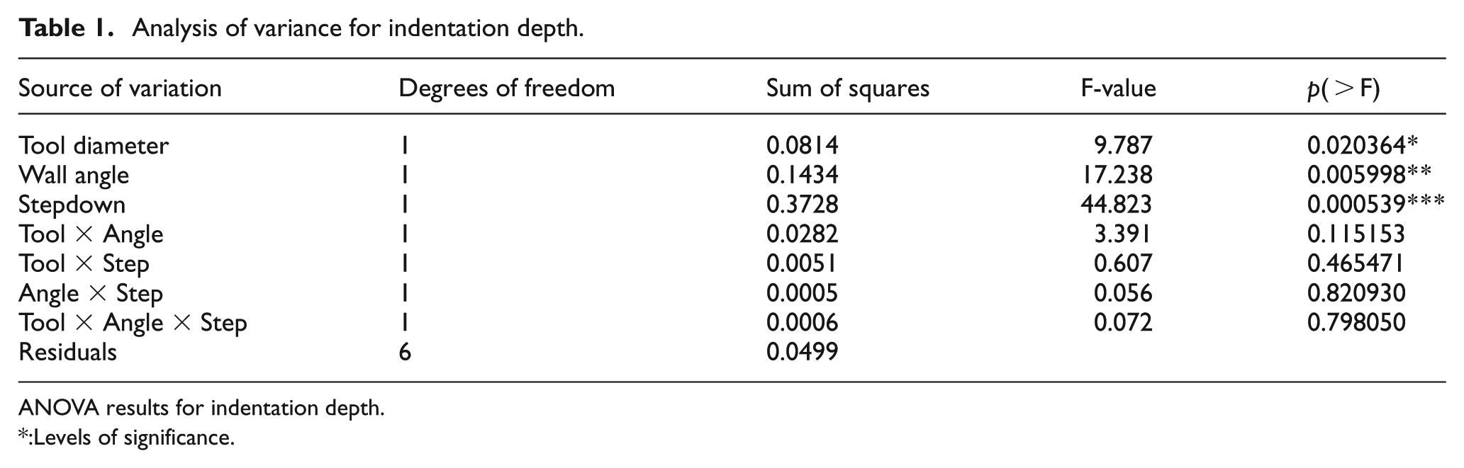
Indentation depth, z_I, was calculated as the difference between tool tip depth and measured bottom plane depth. To determine the contribution of each factor to the depth of indentation, a two-way analysis of variance (ANOVA) was performed using coded variables, the results of which are shown in Table 1. The results show a significant correlation for all three of tool diameter, wall angle and step size, with no significant interactions between factors. A t-test between the centrepoint runs (mean = 0.496, standard deviation (SD) = 0.093) and corner runs (mean = 0.541, SD = 0.300) revealed that there is no significant difference in means to reject the null hypothesis of equal means (t(8.7) = −0.3934, p = 0.70), suggesting that there may not be significant curvature.

Table 1.

Analysis of variance for indentation depth.

Source of variation	Degrees of freedom	Sum of squares	F-value	p(>F)
Tool diameter	1	0.0814	9.787	0.020364*
Wall angle	1	0.1434	17.238	0.005998**
Stepdown	1	0.3728	44.823	0.000539***
Tool × Angle	1	0.0282	3.391	0.115153
Tool × Step	1	0.0051	0.607	0.465471
Angle × Step	1	0.0005	0.056	0.820930
Tool × Angle × Step	1	0.0006	0.072	0.798050
Residuals	6	0.0499

ANOVA results for indentation depth.

*

:Levels of significance.

Using a least squares fit, a linear model is generated to approximate the indentation as a function of tool diameter, wall angle and stepdown, shown in equation (8). Because there were no significant interaction effects found, the model is assumed to be linear. The shape of this function of tool diameter d_t, wall angle φ and stepdown v is shown in Figure 9. For this fit, an R² value of 0.8765 was found.

$$z_I=-0.03177t-0.01339\phi +0.8499v+1.16954$$

(8)

Figure 9.

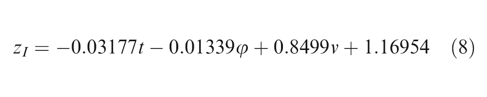
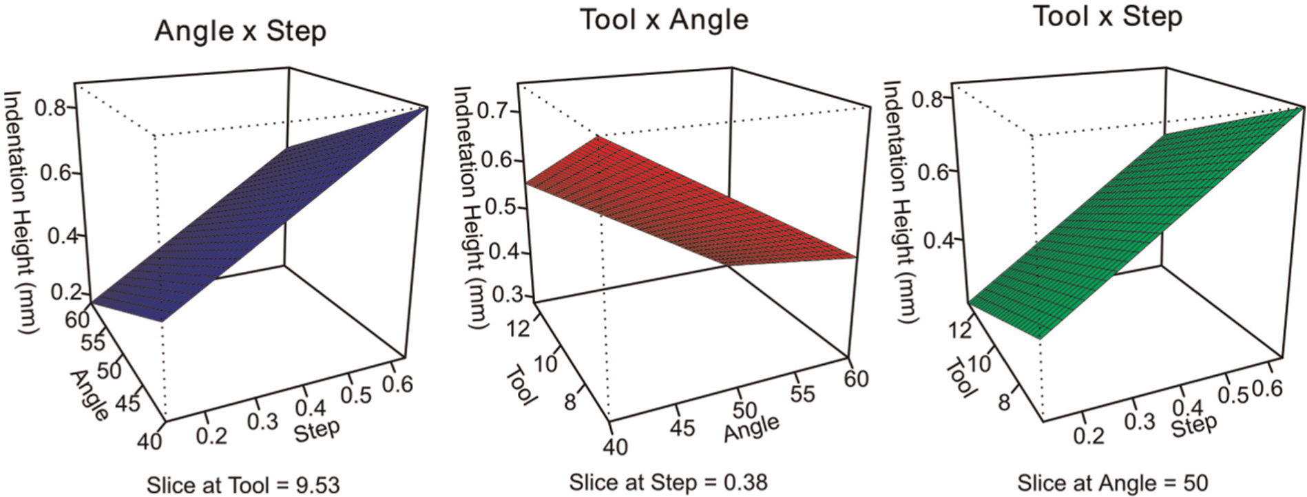
Indentation height as a function of tool diameter, wall angle and stepdown.

The model presented by Aerens, equation (1), predicts that the indentation is a function of the tool diameter only. The experimental results show that indentation depth is in fact dominated by the vertical stepdown, with larger tool diameters reducing the depth of indentation. The negative contribution from tool diameter reflects that larger tools would spread loads over a larger area, reducing indentation.

Trough position

The distance from the tool centre to the trough centre h is a factor that can affect the contact area. As the sample springs back after forming, the trough left by the previous toolpath moves from its ideal position. For a given wall angle, step size and tool diameter, the horizontal position h of the trough relative to the current tool position is ideally given by equation (9)

$$h_{\mathrm{predicted}}=\frac{\mathrm{stepdown}}{\tan \phi }$$

(9)

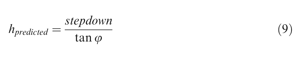
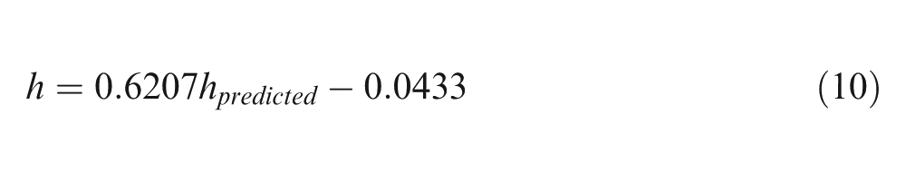
The difference between the predicted value of h and the measured value of h was found to not correlate significantly with any of the three experimental factors used. A least squares fit was used to develop a model to predict true horizontal stepover to the trough based on the predicted stepover and is shown in equation (10). It should be noted, however, that an R² value of 0.583 was reported, suggesting a poor fit. In all tests, however, the measured value of h was less than the value predicted by geometry, indicating that the wall springs inward toward the tool

$$h=0.6207h_{\mathrm{predicted}}-0.0433$$

(10)

Trough diameter

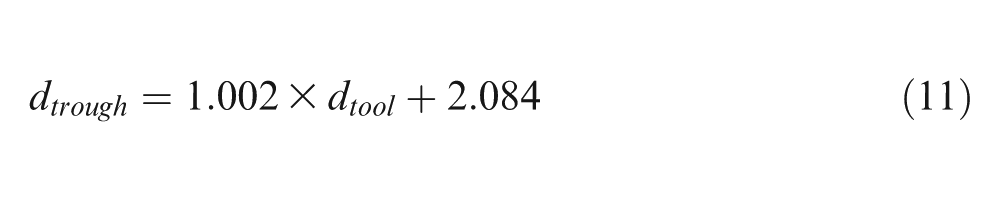
During experimentation, it was observed that the measured troughs were larger than the tool diameters that had made them. An ANOVA revealed that the measured diameter varied only according to the tool diameter used, and a linear regression was performed to fit the trough diameter (Table 2). The regression value for trough diameter d_trough fits the measured data with an R² value of 0.7813

$$d_{\mathrm{trough}}=1.002\times d_{\mathrm{tool}}+2.084$$

(11)

Table 2.

Analysis of variance of trough diameter.

Source of variation	Degrees of freedom	Sum of squares	F-value	p(>F)
Tool diameter	1	81.01	39.919	0.000734***
Wall angle	1	5.72	2.82	0.144121
Stepdown	1	0.44	0.214	0.569612
Tool × Angle	1	1.78	0.876	0.385335
Tool × Step	1	0.05	0.024	0.881257
Angle × Step	1	0.19	0.095	0.768681
Tool × Angle × Step	1	0.14	0.068	0.803123
Residuals	6	12.18

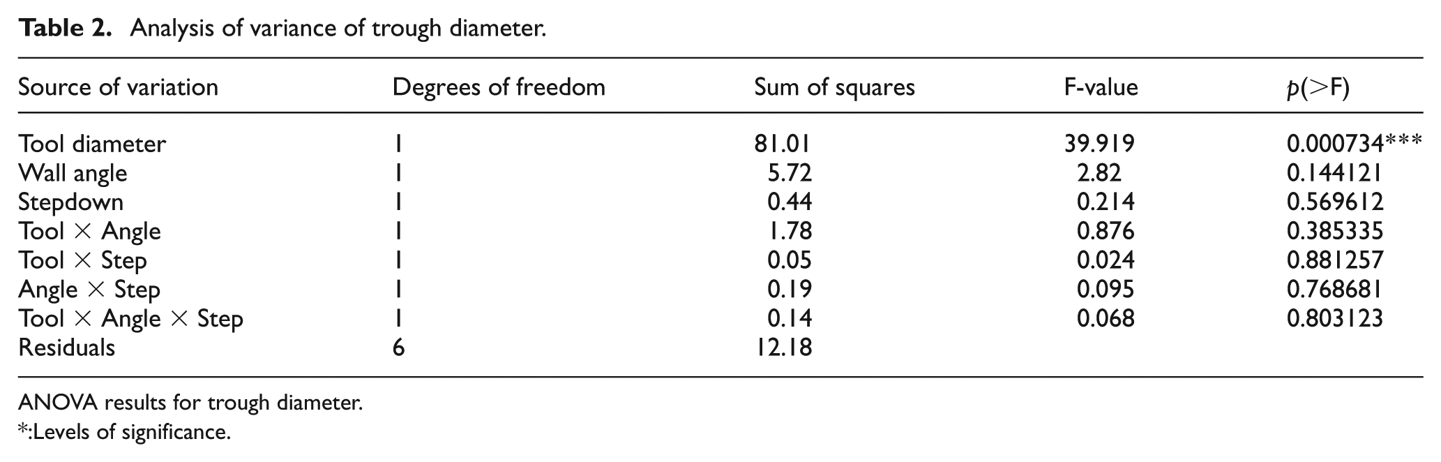
ANOVA results for trough diameter.

*

:Levels of significance.

Because trough diameter change can be explained by springback, it is possible that it is affected by factors not tested, such as part geometry, material and thickness.

Discussion

Trailing trough contribution to area

Upon comparing the height of the trailing trough bottom to the bottom of the tool, it is noticeable that in nearly all cases the bottom of the trough is slightly below the bottom of the tool. When this is coupled with a trough diameter that is larger than the tool, the area contribution is seen to be 0. Images of the contact area agree with this finding, as the leading edge of the contact area tends to be curved with wrap around the front of the tool while the trailing edge is straight. The straight edge is indicative of the sheet remaining in place, and not wrapping around the tool. To calculate the contribution of the trailing edge trough, however, the method above can be repeated.

Horizontal position of trough

The horizontal position of the trough is needed to calculate the contact area and was observed to be less than expected in the ideal case of no springback. To compensate for error in alignment with the machine coordinate system, the position of the trough left by the tool was added to the position of the trough ahead of the tool. The corrected values were therefore the difference between the horizontal positions of the troughs. It should therefore be noted that the error of the corrected values is the sum of error of both left and right trough position measurements. It is likely that this higher error is in part responsible for the poor fit of the trough position values.

Conclusion

A new way of describing contact geometry is presented which describes the shape of contact between the tool and the sheet in SPIF accommodating for tool diameter, wall angle and stepdown. This method allows contact area to be determined based on directly measurable features, thereby allowing empirical models to be developed and analytical models to be tested.

To test the contributions of tool diameter, wall angle and stepdown on contact area, a series of samples were formed. Using measurements taken with a CMM probe, the area of contact was calculated for each part. Indentation was found to vary according to all three of tool diameter, step size and wall angle, though most substantially along step size. The total contact area was also found to be affected by all three of the factors studied, however most dramatically as a factor of tool diameter.

In all samples formed, the trough diameter was larger than the tool and closer to the tool than the previous programmed toolpath. The larger trough diameter may be explained by the bottom of the sample attempting to flatten out, while the closer trough centre may be explained by bending of the wall toward the centre.