Cut quality assessment of CO 2 laser cutting of twinning-induced plasticity steel sheets

Abstract

In this study, the effects of the main process parameters involved in CO₂ laser cutting of 1.5-mm twinning-induced plasticity steel sheets have been investigated by means of experimental tests. The quality of the cut edges of the sheets was evaluated by analyzing the kerf width, kerf deviation, roughness of the cut surfaces, and dross attachment. The process parameters used were the laser power, cutting speed, oxygen pressure, and pulse frequency of the CO₂ laser beam. The optimal settings of the process parameters were predicted using the Taguchi parameter design approach with an L27(3¹³) orthogonal array and calculating the average effect of both the laser parameters and the signal-to-noise ratios. Analysis of variance was performed to evaluate the statistical significance and the contribution of the laser process parameters to the examined kerf features and roughness. On the basis of the Taguchi approach, the predicted optimal settings of the process parameters were verified through confirmation tests. The results show that the selected process parameters, as well as their interactions, can have a remarkable effect on the cutting quality of twinning-induced plasticity steel sheets. The laser power is the main process parameter that affects the kerf width on both sheet sides, while the pulse frequency and its interaction with the laser power are the main factors that influence the kerf deviation, followed by the cutting speed. The roughness of the cut surfaces is mainly affected by the oxygen pressure and the interaction between laser power and cutting speed. Dross attachment was primarily observed in the specimens cut with high laser power and low cutting speed.

Introduction

The CO₂ laser beam is increasingly used in manufacturing engineering to cut steel sheets into appropriate shapes, with the process parameters being chosen accurately to obtain good quality of the cut surfaces. The cutting process is obtained from the thermal energy supplied by a laser beam that moves on a sheet surface along an appropriate tool path, previously set in a laser machine (as done on a traditional computer numerical control machine). Laser cutting, being a contactless process, does not use any traditional cutting tools and, hence, no direct mechanical cutting forces are applied to the sheets that have to be cut. In a gas-assisted cutting process, steel sheets can be cut by means of either gas-assisted fusion cutting or reactive gas-assisted cutting. In the former case, a CO₂ laser beam is focused on the sheet surface, so that the metal melts; an inert flowing gas (such as argon or nitrogen) then removes the molten material. In the latter case, an assist gas, usually oxygen, also exothermally reacts with the metal, thus enhancing the thermal energy that is available for the cutting process.

As the front edge of the cut can be slightly inclined from the vertical and the laser beam usually has a converging–diverging shape, the kerf width on the top and bottom sides of the cut sheets is not the same; therefore, a kerf taper always occurs. The other main issues related to the quality of laser cut steel sheets are kerf deviation, resolidified layers, adhesion of dross, surface oxidation, heat-affected zones, out of flatness, and striation patterns on the cut surfaces. Sideways burning and excessive mass removal from the kerf may also occur due to the high temperature that is reached during the cutting process, especially if an exothermic reaction takes place between the assist gas and metal sheet. For these reasons, an appropriate selection of the laser cutting parameters is necessary to control these defects. Moreover, the precision of the laser cut and, hence, the dimensional accuracy are very important as they help to ensure correct part tolerances and fit-up, thus avoiding secondary processing and rework operations.

The most important process parameters involved in laser cutting include the type and power of the laser beam, cutting speed, type and pressure of the assist gas, and the mode of operation of the laser beam (pulsed or continuous). ¹ These parameters are set according to the type of the steel grade and the sheet thickness to be cut.

CO₂ laser cutting is considered a feasible alternative to mechanical cutting and blanking due to its flexibility and ability to process sheet metal parts in a very short time and with minimal waste. For these reasons, CO₂ laser cutting is increasingly adopted to cut steel sheets in the automotive industry. Over the last few years, new high-manganese austenitic steels, known as twinning-induced plasticity (TWIP), have increasingly been the subject of particular attention in the automotive industry due to their excellent combination of strength and ductility, and proposed for the manufacturing of car body components through sheet-forming operations. Fracture elongation superior to 50% and tensile strength higher than 1000 MPa are usually obtained because of the formation of mechanical twins during plastic deformation.^2–4 Automotive sheet components in TWIP steels are still under development, and, unless rare cases, only prototypal components have been fabricated so far. Many experimental and theoretical studies have already been carried out to analyze the effects of laser process parameters on both the kerf features and cut surface quality of conventional steel grades,^5–8 stainless steels,^9,10 aluminum alloys,^11,12 and titanium alloys.^13–15 However, these investigations have not been conducted on high-manganese steel grades so far, such as TWIP and Hadfield ones. Several design of experiment methods have been used to examine and optimize laser cutting operations.^16–19 In particular, the Taguchi approach has proved very useful to offer an empirical and simple methodology to evaluate the optimal laser parameter settings and, hence, to ensure an appropriate cut quality.^20,21

In this study, the effects of pulsed CO₂ laser cutting parameters on the cut edge quality of 1.5-mm-thick TWIP steel sheets have been investigated through experimental tests. The used process parameters were laser power, cutting speed, oxygen pressure, and pulse frequency of the laser beam. A design of experiments was adopted according to the Taguchi quality design approach. Kerf width, on both sides of the cut metal sheets, kerf deviation, on the side where the laser beam first hits the sheet, and the total height of the roughness profile of the cut surfaces were measured in order to evaluate the cut edge quality of the TWIP steel sheets. The dross attachment on the bottom edges was assessed based on three classes of cuts.

An analysis of variance (ANOVA) was performed on the kerf features and roughness values in order to evaluate the statistical significance and the contribution of each process parameter, as well as the interactions between the laser power and the other process parameters. The Taguchi approach was also used to predict the optimal combinations of the cutting parameters and, hence, to maximize the cut edge quality of the TWIP steel sheets, in terms of kerf width, kerf deviation, and roughness. Finally, these optimal combinations were verified through confirmation tests.

Taguchi method for process parameters design

The Taguchi method is one of the most important approaches used to design manufacturing process parameters through the implementation of a robust design of experiments. It is a statistical experimental design technique that is used to evaluate several design parameters simultaneously, at different levels, with the aim of predicting an optimal combination of these parameters and, hence, of obtaining desired output responses. It is highly effective in reducing the number of experiments, which would otherwise be needed in a full factorial analysis. In such a sense, an orthogonal array containing the control factor (process parameter) settings is used to systematically vary and test the different levels of each control factor, as well as its interactions with the other process parameters. An orthogonal array is a matrix in which each column indicates a control factor, or an interaction, and its corresponding levels, while each row represents an experimental trial that is performed at the given control factor settings. The dimension of this matrix varies according to the number of the process parameters and levels involved; when nonlinear effects are expected, more than two levels of the factors are better. ²² In this regard, a complete list of orthogonal arrays can be found in the literature. ²³ The estimated mean value of the output response at the optimal condition, m_opt, is computed by adding all the improvements (contributions) from all the control factors to the average of all the trial results (grand average performance, $\stackrel{·}{\text{T}}$ ). ²⁴ Thus, m_opt can be calculated as follows

$${\text{m}}_{\text{opt}}=\stackrel{·}{\text{T}}+\sum _1^{\text{k}}({\text{m}}_{{\text{m}}_{\text{i}}}-\stackrel{·}{\text{T}})$$

(1)

where k is the number of significant control factors obtained from an ANOVA carried out on the output responses, and ${\text{m}}_{{\text{m}}_{\text{i}}}$ is the average mean for ith control factor corresponding to the optimal factor level, according to the desired performance response. However, when a significant interaction exists, especially when its effect is larger than that of the control factors, equation (1) should include at first the average mean of the interaction to the optimal factor level and then those of the remaining significant control factors (excluding the process parameters already considered in the interaction). ²⁴

Although the above-mentioned calculation is quite simple, it might not capture the variability of data within the examined control factors. A better way of comparing population behavior is to use the mean-squared deviation (MSD) of the output results. For linearity convenience and in order to accommodate wide-ranging data, a log transformation of MSD, known as the signal-to-noise (S/N) ratio, is recommended for the analysis of experimental results. ²² In this way, the optimal parameter settings can be predicted from the factor levels that maximize the S/N ratio. There are three standard types of S/N ratio (expressed in a decibel scale), depending on the desired performance response, so defined: ²⁵

• Smaller the better, for making the system response as small as possible

  $$\text{S}/{\text{N}}_{\text{S}}=-10\text{log}[\text{MSD}]=-10\text{log}\left[\left(\frac{1}{\text{n}}\right)\sum _1^{\text{n}}{\text{y}}_{\text{i}}^2\right]$$

  (2)

• Nominal the best, for reducing variability around a target

  $$\text{S}/{\text{N}}_{\text{N}}=10\text{log}[\text{MSD}]=10\text{log}\left(\frac{{\overline{\text{y}}}^2}{\text{S}{\text{D}}^2}\right)$$

  (3)

• Larger the better, for making the system response as large as possible

$$\text{S}/{\text{N}}_{\text{L}}=-10\text{log}[\text{MSD}]=-10\text{log}\left[\left(\frac{1}{\text{n}}\right)\sum _1^{\text{n}}\left(\frac{1}{{\text{y}}_{\text{i}}^2}\right)\right]$$

(4)

where $\overline{\text{y}}$ is the mean output response, and SD is the standard deviation of each experimental trial. They are computed using the following formulas

$$\overline{\text{y}}=\left(\frac{1}{\text{n}}\right)\sum _1^{\text{n}}{\text{y}}_{\text{i}}$$

(5)

$$\text{SD}={\left\{\sum _1^{\text{n}}[{({\text{y}}_{\text{i}}-\overline{\text{y}})}^2/\text{n}]\right\}}^{1/2}$$

(6)

where y_i is the experimental measured value of the examined feature for the ith experimental trial, and n is the total number of the experimental trials at the same levels of process parameter. Once all of the S/N ratios have been computed for each experimental trial, a graphical approach can be used to analyze the data, that is, the S/N ratios and average responses are plotted for each control factor against each of its levels. The graphs are then examined in order to find the pick factor levels that best maximize the S/N ratio and ensure that the mean is on target, or maximize or minimize the mean, as the case may be. In an S/N approach, the estimated mean value of the response at the optimal condition is also calculated using equation (1); in this way, ${\text{m}}_{{\text{m}}_{\text{i}}}$ and m_opt are expressed in terms of the S/N ratio. The optimal S/N ratio is then back-transformed to find the MSD, and from the MSD to estimate the expected result. As equations (2)–(4) involve unknown variables (y_i), only an approximate solution of the expected result can be obtained if it is assumed that all the results (y_i) are expected to be the same as their representative value, Y_exp. ²² The following formulas are used depending on the desired performance response

$$\text{Smaller the better}:{\text{Y}}_{\text{exp}}=\text{MS}{\text{D}}^{1/2}$$

(7)

$$\text{Nominal the best}:{\text{Y}}_{\text{exp}}={\text{Y}}_0\pm \text{MS}{\text{D}}^{1/2}$$

(8)

$$\text{Larger}\text{the better}:{\text{Y}}_{\text{exp}}=\frac{1}{(\text{MS}{\text{D}}^{1/2})}$$

(9)

where Y₀ is the target value in the “nominal the best” condition.

An interval can be set around the mean value at the optimal parameter level, and a range of values can thus be defined within which the true average of the response would be expected to fall with a certain confidence. This range is

$${\text{m}}_{\text{opt}}-\text{CI}<{\text{m}}_{\text{opt}}<{\text{m}}_{\text{opt}}+\text{CI}$$

(10)

and

$${\text{Y}}_{\text{exp}}-\text{CI}<{\text{Y}}_{\text{exp}}<{\text{Y}}_{\text{exp}}+\text{CI}$$

(11)

for the average effect of the parameters and the S/N ratio analysis, respectively. The extent of confidence interval (CI) of confirmation experiments is found by the following formula ²²

$$\text{CI}={\{{\text{F}}_{\text{α}}(1,{\text{f}}_{\text{e}}){\text{V}}_{\text{e}}[\frac{1}{{\text{N}}_{\text{ef}}}+\frac{1}{\text{R}}]\}}^{1/2}$$

(12)

where F_α(1, f_e) is the F-ratio at a confidence level (1 −α) against 1 degree of freedom (dof) with an error f_e, V_e is the error variance (error mean square), R is the sample size of the confirmation experiment, and N_ef is the effective number of replications, so calculated

$$\begin{array}{c}{\text{N}}_{\text{ef}}=\frac{\text{N}}{(1+\text{dof of total factors included in estimating the}{\text{m}}_{\text{opt}}\text{or}{\text{Y}}_{\text{exp}})}\hfill \end{array}$$

(13)

with N being the total number of the experiments (number of trials multiplied by number of replications).

Confirmation tests are performed using the previously evaluated optimal combinations of the control factors and levels. These tests have the aim of establishing the performance at the optimal conditions and of determining and, hence, of validating, how close the predicted optimal performance is to the observed results. ²⁶

Material and experimental procedure

A set of 1.5 (±0.05)-mm-thick TWIP steel sheets was selected for this work. The chemical composition and the main mechanical properties of the sheets are shown in Table 1. The sheet samples were previously cut into a square shape by shearing, the final dimension being around 350 mm × 350 mm. These specimens were then cleaned in order to remove dust before the experimental laser cutting tests.

Table 1.

Chemical composition and main mechanical properties of the examined TWIP steel sheets.

Chemical composition a (wt%)		Mechanical properties
Carbon	0.51	Yield strength	460 MPa
Manganese	22.4	Tensile strength	1005 MPa
Molybdenum	0.70	Elongation at fracture	45%
Vanadium	0.22	Vickers hardness	270 HV30

a

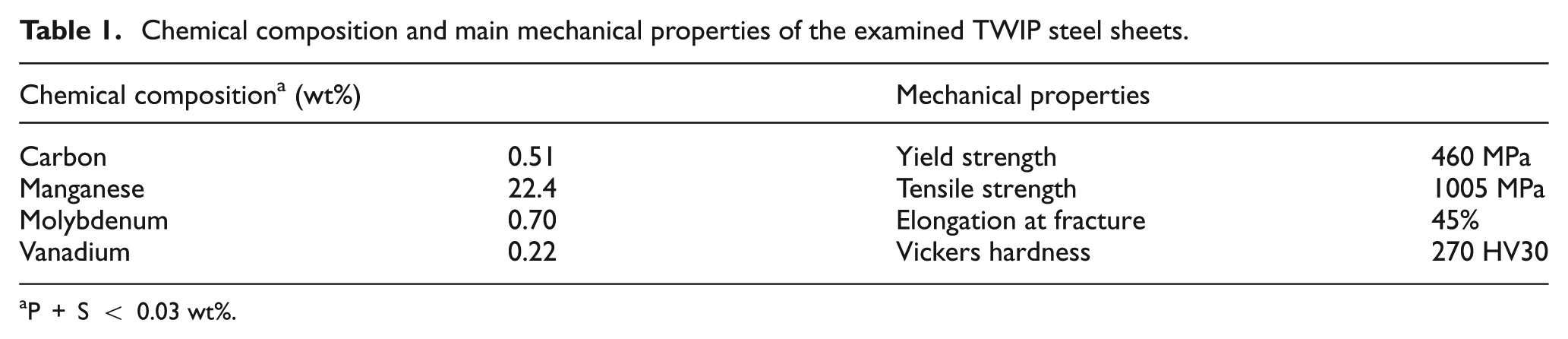
P + S < 0.03 wt%.

The experimental laser cutting tests were carried out using a CO₂ laser machine with oxygen as the assist gas. The laser beam was generated from a pulsed CO₂ laser source with a maximum power of 350 W. The laser beam was transferred from the generation source to the workpiece through an optic fiber path. The cutting head of the laser machine was mounted on a three-axis mechanical device. The movements along the x, y, and z axes were performed by means of linear motors, with the Cartesian coordinates and position being controlled by optical encoders. The cutting head was also equipped with a servo motor and electrostatic sensor to automatically adjust the stand-off distance during the laser cutting operations (since the steel sheets were not perfectly planar). The cutting parameters were set on the laser machine by means of a digital controller.

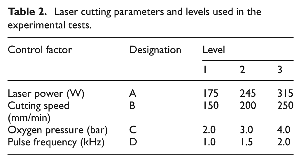
Oxygen was flowed coaxially with the laser beam through a nozzle with an outlet diameter of 1.5 mm. The laser beam of 0.2 mm spot size was focused using a 95-mm focal length lens, with a stand-off distance of 1 mm to have the focal point within the sheet thickness. The workpiece thickness, nozzle diameter, stand-off distance, spot size of the laser beam, and focal length of the lens were maintained constant for all the tests. The cutting parameters were laser power, cutting speed, oxygen pressure, and pulse frequency of the CO₂ laser beam. A previous pilot experiment was performed in order to define the process parameters range for the laser cutting tests. Three levels of each control factor were selected for the experimental tests (Table 2). The minimum pulse frequency of the laser beam and cutting speed were chosen to have two neighbor laser spots on material surface that overlapped at least 80%, thereby ensuring proper cutting operations. ²⁷ According to the range of the pulse frequency values, each laser pulse lasted from 0.5 to 1 ms.

Table 2.

Laser cutting parameters and levels used in the experimental tests.

Control factor	Designation	Level
		1	2	3
Laser power (W)	A	175	245	315
Cutting speed (mm/min)	B	150	200	250
Oxygen pressure (bar)	C	2.0	3.0	4.0
Pulse frequency (kHz)	D	1.0	1.5	2.0

The Taguchi approach was used to evaluate the influence of the laser process parameters, as well as the interactions between the laser power (considered as the main factor of influence on the cutting operations) and the other parameters, on cut edge quality. An L27(3¹³) orthogonal array (consisting of 27 rows and 13 columns) was used to design the experimental tests (Table 3).

Table 3.

Taguchi L27(3¹³) orthogonal array with the examined control factors and interactions (raw and S/N ratio data).

Trial	Factor level
	A	B	A×B	A×B	C	A×C	A×C	A×D	D	A×D	–	–	–
1	1	1	1	1	1	1	1	1	1	1	1	1	1
2	1	1	1	1	2	2	2	2	2	2	2	2	2
3	1	1	1	1	3	3	3	3	3	3	3	3	3
4	1	2	2	2	1	1	1	2	2	2	3	3	3
5	1	2	2	2	2	2	2	3	3	3	1	1	1
6	1	2	2	2	3	3	3	1	1	1	2	2	2
7	1	3	3	3	1	1	1	3	3	3	2	2	2
8	1	3	3	3	2	2	2	1	1	1	3	3	3
9	1	3	3	3	3	3	3	2	2	2	1	1	1
10	2	1	2	3	1	2	3	1	2	3	1	2	3
11	2	1	2	3	2	3	1	2	3	1	2	3	1
12	2	1	2	3	3	1	2	3	1	2	3	1	2
13	2	2	3	1	1	2	3	2	3	1	3	1	2
14	2	2	3	1	2	3	1	3	1	2	1	2	3
15	2	2	3	1	3	1	2	1	2	3	2	3	1
16	2	3	1	2	1	2	3	3	1	2	2	3	1
17	2	3	1	2	2	3	1	1	2	3	3	1	2
18	2	3	1	2	3	1	2	2	3	1	1	2	3
19	3	1	3	2	1	3	2	1	3	2	1	3	2
20	3	1	3	2	2	1	3	2	1	3	2	1	3
21	3	1	3	2	3	2	1	3	2	1	3	2	1
22	3	2	1	3	1	3	2	2	1	3	3	2	1
23	3	2	1	3	2	1	3	3	2	1	1	3	2
24	3	2	1	3	3	2	1	1	3	2	2	1	3
25	3	3	2	1	1	3	2	3	2	1	2	1	3
26	3	3	2	1	2	1	3	1	3	2	3	2	1
27	3	3	2	1	3	2	1	2	1	3	1	3	2

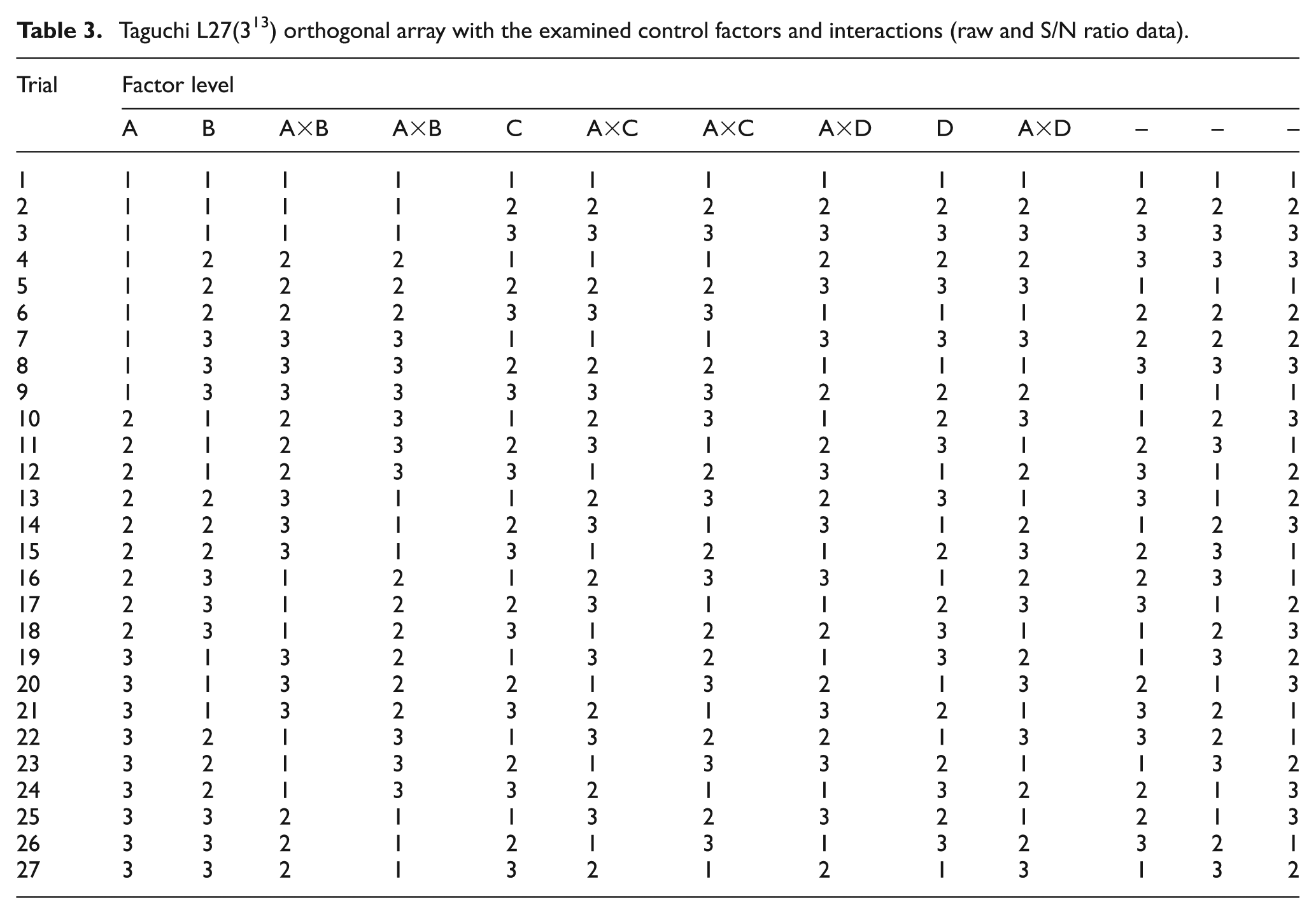
Twenty-seven combinations were implemented, with each factor level occurring for the same number of times (balancing property). The triangular table proposed by Taguchi et al. ²³ was used to determine the columns reserved for the analysis of the examined process parameters and interactions. Each control factor was assigned to columns 1, 2, 5, and 9, while the interactions were assigned to columns 3 and 4 (interaction between the laser power and the cutting speed, A×B), 6 and 7 (interaction between the laser power and the oxygen pressure, A×C), and 8 and 10 (interaction between the laser power and the pulse frequency, A×D). The unassigned columns were not used in the ANOVA. Numbers 1–3 in the L27(3¹³) array stand for the levels 1–3 listed in Table 2.

Cut quality was evaluated in terms of kerf width, kerf deviation, roughness, and dross attachment for all the experimental trials, according to the combination of the control factor levels listed in Table 3. Three replications were made for each trial in order to achieve consistent results; thus, 81 laser cutting operations were performed overall. Kerf width was evaluated on both sides of the TWIP steel sheets (Figure 1). The top kerf width, Kw_t, and the bottom kerf width, Kw_b, were measured by means of an optical microscope at 10× magnification along the cut path.

Figure 1.

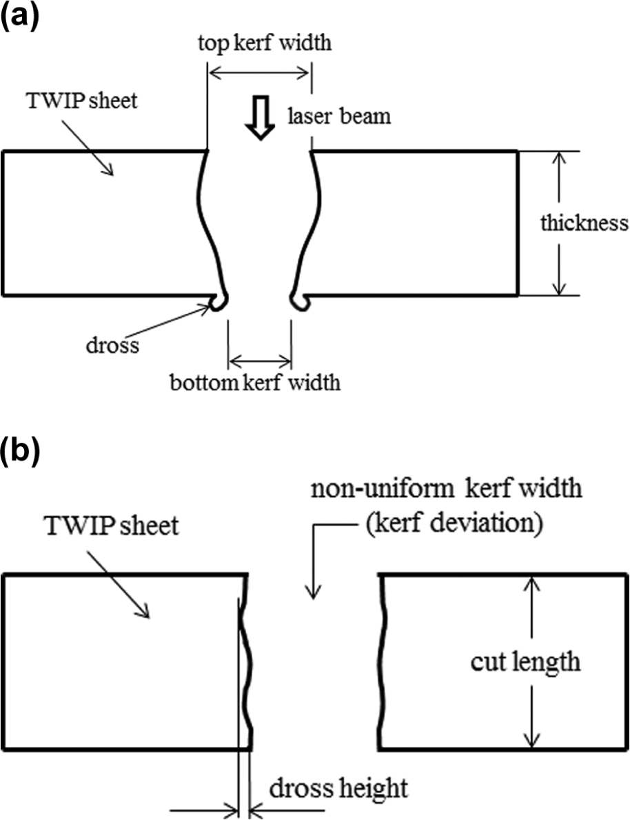
Schematic illustration of the laser cut TWIP steel sheet: (a) kerf along sheet cross section and (b) kerf deviation along the cut direction.

The measurement procedure used to evaluate kerf width was as follows: optical micrographs were taken in five different zones spaced equally along the cut path. Four kerf width values were extracted by each micrograph, considering two maximum and two minimum distances between the opposite cut edges (see white lines in Figure 2). The 20 measurements obtained were then averaged in order to evaluate kerf width. This measurement procedure was performed on both the top and bottom kerf width and repeated for all the three replications. The kerf deviation was calculated as the difference between the maximum and the minimum kerf width measured on the top sheet surface (considering all the replications)

$$\text{D}{\text{h}}_{\text{t}}=\text{maximum}\text{K}{\text{w}}_{\text{t}}-\text{minimum}\text{K}{\text{w}}_{\text{t}}$$

Figure 2.

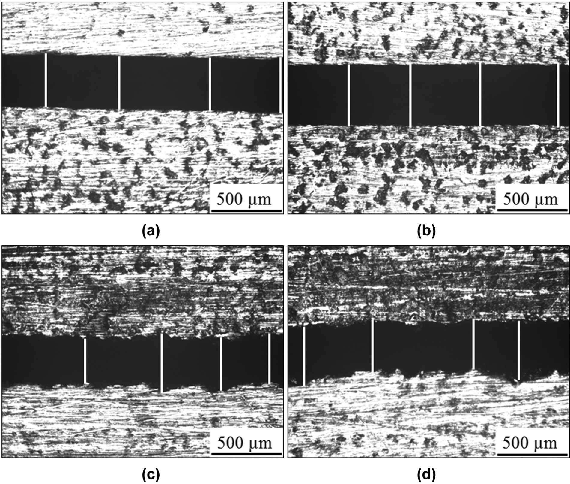
Optical micrographs of kerf after laser cutting: (a, c) trial 4 and (b, d) trial 25. (a, b) Top edges and (c, d) bottom edges.

The roughness profile of the cut surfaces was measured in the middle of the sheet thickness by means of a high-precision inductive stylus instrument. The total height of the roughness profile, Rt, was used to evaluate the maximum peak-to-valley distance of the striations on the cut surfaces.

Based on a previous study, ²⁸ the dross attachment was classified into three classes of cuts: Class I, dross deposition with an excess of material removed at the bottom of the cut surfaces; Class II, dross deposition with flat cut surfaces; Class III, no or minimum dross deposition with flat cut surfaces. The ends of the cut edges, which indicate the beginning and the end of the cutting zone, were excluded in the measurement of the kerf features and roughness profiles and for dross assessment.

The statistical significance and the corresponding contribution of each control factor or interaction on the kerf features and roughness were obtained by means of ANOVA. ANOVA decomposes the variability of the kerf features and roughness values into contributions due to various factors with respect to the overall measured values. The laser cutting parameters and their interactions were considered to have a statistically significant effect on the kerf features and Rt values at a 90% confidence level.

Results and discussions

Experimental results

The kerf width and roughness values obtained from each experimental trial are shown in Table 4. As smaller kerf width, kerf deviation, and roughness values were desired to obtain high-quality cut surfaces, the S/N_S ratio was computed with equation (2). A small kerf width allows a minimum amount of material to be melted and hence thermal energy to be used efficiently. The types of dross deposition on the bottom edges are also listed in Table 4, according to the three classes of cuts.

Table 4.

Mean values of the kerf features and Rt: raw data and S/N_S ratios (smaller the better performance).

Trial	Factor level				Class of cut	Raw data				S/NS ratio
	A	B	C	D		Kwt (mm)	Kwb (mm)	Dht (mm)	Rt (µm)	Kwt (dB)	Kwb (dB)	Dht (dB)	Rt (dB)
1	1	1	1	1	III	0.399	0.246	0.093	18.73	7.98	12.18	20.63	−25.45
2	1	1	2	2	III	0.424	0.250	0.080	19.31	7.46	12.05	21.94	−25.71
3	1	1	3	3	III	0.369	0.266	0.022	24.36	8.66	11.49	33.15	−27.73
4	1	2	1	2	III	0.407	0.222	0.104	24.16	7.82	13.08	19.66	−27.66
5	1	2	2	3	III	0.372	0.232	0.018	29.30	8.58	12.70	34.89	−29.34
6	1	2	3	1	III	0.406	0.236	0.060	33.67	7.83	12.55	24.44	−30.54
7	1	3	1	3	III	0.353	0.204	0.023	22.11	9.04	13.79	32.77	−26.89
8	1	3	2	1	III	0.443	0.230	0.024	20.78	7.06	12.75	32.40	−26.35
9	1	3	3	2	III	0.464	0.234	0.090	21.82	6.67	12.62	20.92	−26.78
10	2	1	1	2	II	0.440	0.251	0.032	15.44	7.13	12.01	29.90	−23.77
11	2	1	2	3	II	0.453	0.200	0.060	23.30	6.87	13.99	24.44	−27.35
12	2	1	3	1	II	0.483	0.260	0.049	24.86	6.32	11.71	26.20	−27.91
13	2	2	1	3	II	0.446	0.224	0.039	17.00	7.02	13.00	28.18	−24.61
14	2	2	2	1	II	0.419	0.268	0.054	18.78	7.56	11.45	25.35	−25.47
15	2	2	3	2	II	0.424	0.251	0.048	16.42	7.45	12.00	26.38	−24.31
16	2	3	1	1	III	0.452	0.233	0.016	17.56	6.89	12.66	35.92	−24.89
17	2	3	2	2	III	0.395	0.259	0.029	37.64	8.07	11.72	30.75	−31.51
18	2	3	3	3	III	0.417	0.210	0.025	43.65	7.60	13.54	32.04	−32.80
19	3	1	1	3	II	0.484	0.291	0.038	17.61	6.30	10.72	28.40	−24.92
20	3	1	2	1	II	0.472	0.294	0.029	20.97	6.52	10.63	30.75	−26.43
21	3	1	3	2	II	0.506	0.242	0.101	40.18	5.92	12.34	19.91	−32.08
22	3	2	1	1	II	0.442	0.290	0.032	14.46	7.10	10.74	29.90	−23.20
23	3	2	2	2	II	0.456	0.277	0.046	20.97	6.81	11.14	26.74	−26.43
24	3	2	3	3	III	0.487	0.256	0.061	28.66	6.24	11.84	24.29	−29.15
25	3	3	1	2	II	0.421	0.255	0.048	31.45	7.52	11.87	26.38	−29.95
26	3	3	2	3	III	0.440	0.231	0.028	42.61	7.13	12.71	31.06	−32.59
27	3	3	3	1	III	0.440	0.249	0.020	47.38	7.14	12.06	33.98	−33.51
Grand average performance, ${\text{m}}_{{\text{m}}_{\text{i}}}$						0.434	0.247	0.047	25.67	7.28	12.20	27.83	−27.68

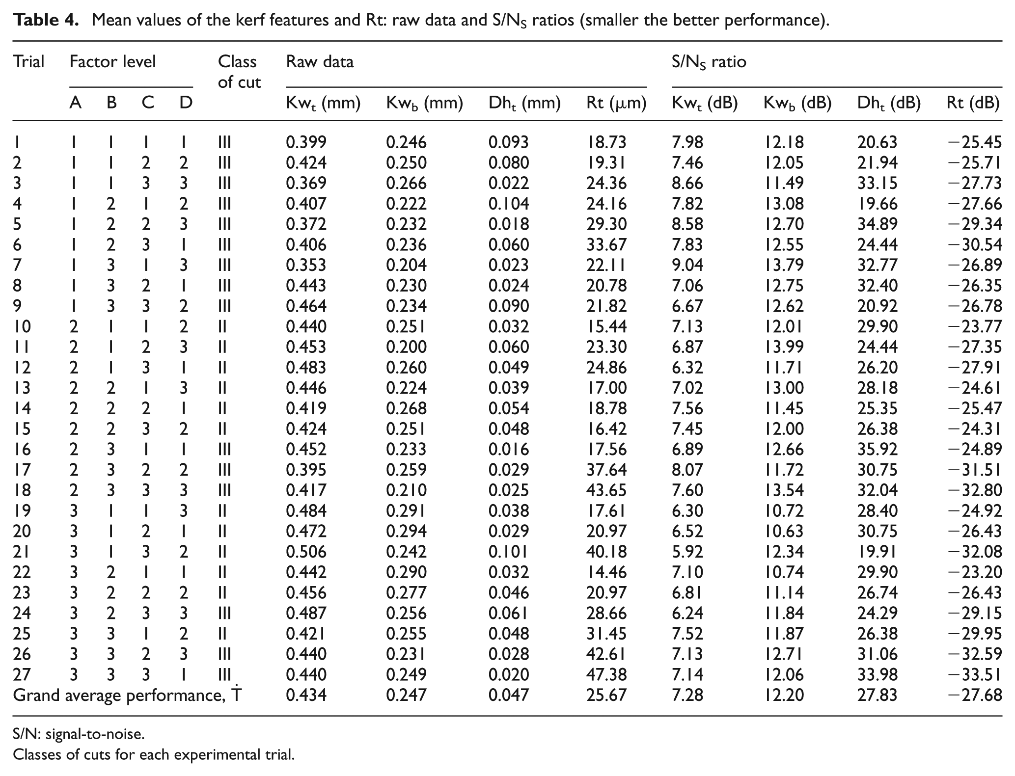
S/N: signal-to-noise.

Classes of cuts for each experimental trial.

The variability of the results of each test was analyzed in order to evaluate the expanded uncertainty of the kerf width values. Thus, the average variances of the kerf width values were calculated and then compared each other using Pearson’s test, which allows the data to be considered homoscedastic. The corresponding standard deviation values were put as reproducibility into the uncertainty table, according to the standard ISO/IEC Guide 98-3:2008. ²⁹ From this analysis, the effects of the bias and of the resolution of the instrument were negligible. The resulting expanded uncertainty for kerf width measurements was 0.024 mm.

Visual examination of the kerfs reveals that the top edges have quite regular profile, regardless of the process parameters used (Figure 2(a) and (b)). The bottom edges, instead, exhibit irregular profiles due to the ejection of the molten material (Figure 2(c) and (d)), especially when dross attachment occurs (class of cut II).

Depending on the process parameters used, different striation patterns can be seen under optical microscopy examination (Figure 3). Low laser power and cutting speed promote the formation of quite regular striation patterns with short peak-to-valley distances (Figure 3(a) and Table 4). This is mainly due to the lower thermal energy supplied per unit time to the sheet during the cutting process. As well known, on increasing the cutting speed, the striations tend to curve from the top to the bottom of the cut surfaces, and in opposite direction in respect to the movement of the laser torch (Figure 3(b)). Moreover, it can be noted that the cut surfaces appear more irregular, thereby exhibiting higher Rt values (Table 4). Sideways burning seems to be the cause for the formation of striation patterns on the cut surfaces. During the cutting process, the instability of the molten material along the cut front ³⁰ and the possible small fluctuations occurring in laser power and gas flow ³¹ might also sustain the formation of the striations.

Figure 3.

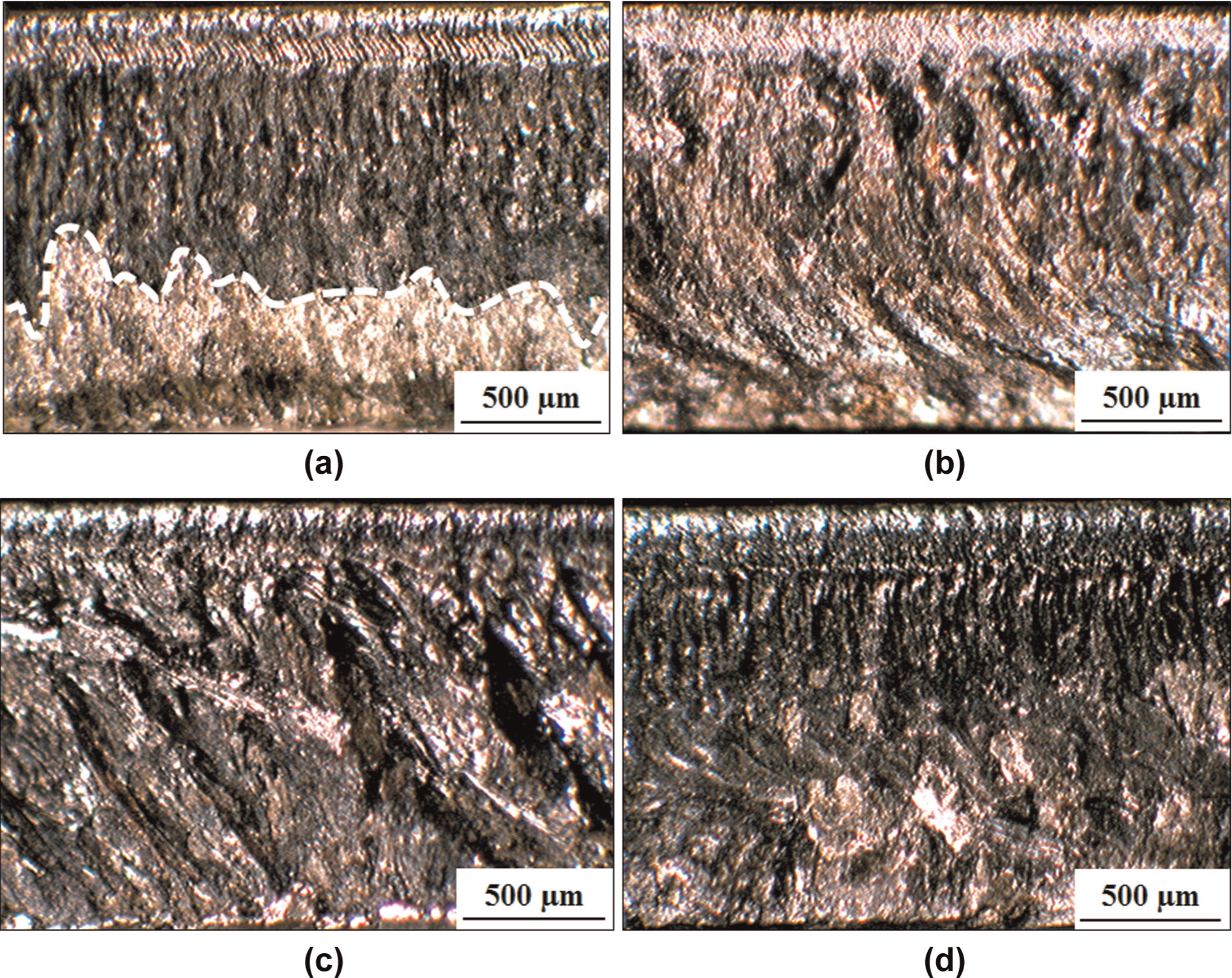
Optical micrographs of the cut surfaces obtained at different laser cutting conditions: (a) trial 1 (the oxide layer is detached in the area below the dotted line), (b) trial 9, (c) trial 18, and (d) trial 27.

There is no clear relationship among kerf width, roughness of the cut surfaces, and dross attachment. In fact, the cut specimens that show small kerf widths and the absence of dross attachment can exhibit irregular roughness profiles and higher Rt values (Figure 3(c) and (d) and Table 2). The relationship between the cut surface appearance and roughness is well defined by the scanning electron microscope (SEM) photographs and the corresponding roughness profiles of Figure 4.

Figure 4.

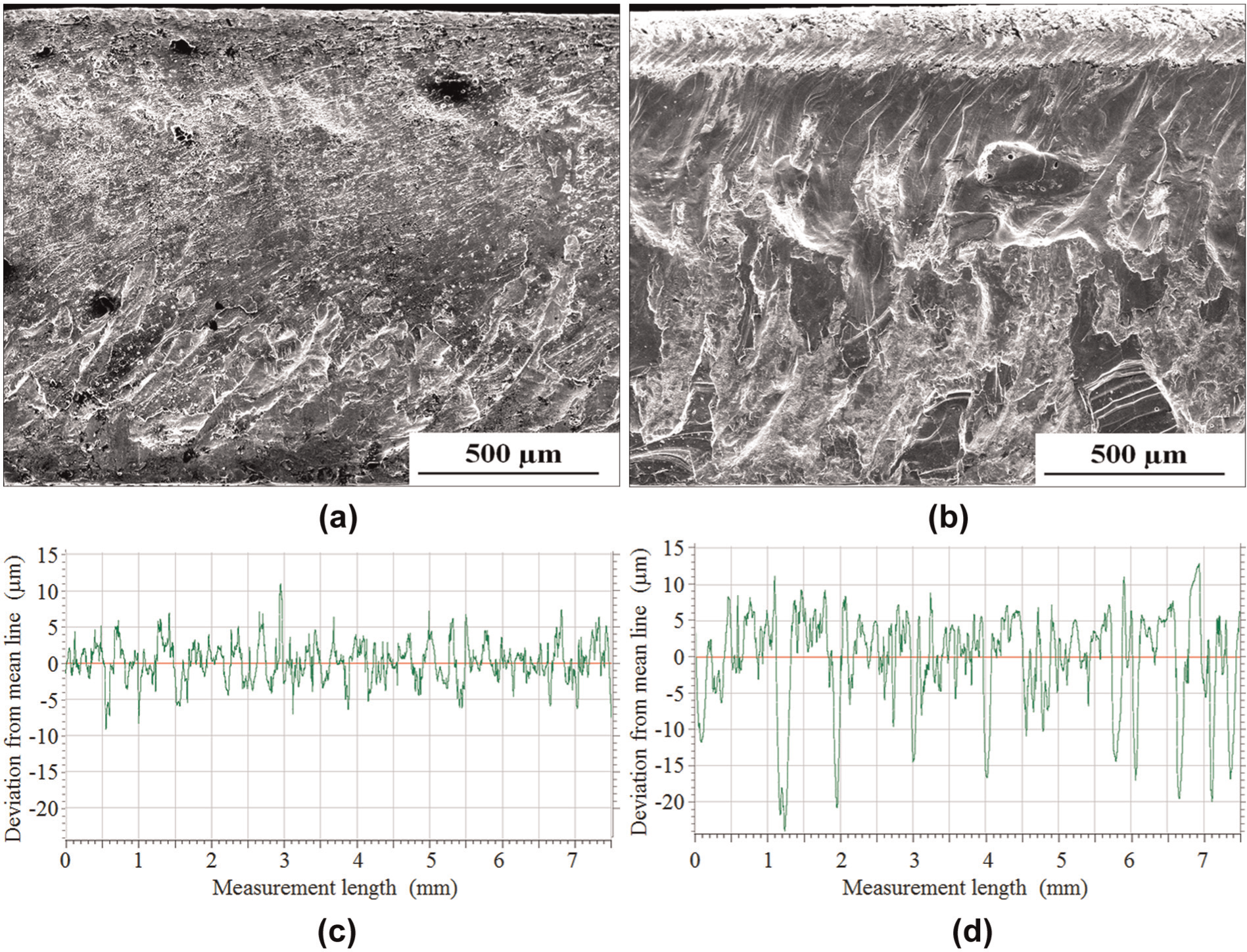
SEM photographs of (a) flat and (b) irregular cut surfaces; the respective roughness profiles are depicted in (c) and (d). (a, c) Trial 4 and (b, d) trial 17.

The formation of dross deposition in gas-assisted laser cutting is mainly associated with the increase in viscosity of the molten material that moves from the top to the bottom of the cut surface (which increases due to the cooling effect of the assist gas), followed by melt solidification on the side walls. In this study, the dross attachment is primarily affected by the laser power and cutting speed. Indeed, the dross attachment was absent when the laser power was at level 1 (175 W), regardless of the level of the other process parameters. When the laser power was at levels 2 (245 W) and 3 (315 W), the dross deposition was usually detected only if low and medium cutting speeds were used. In these conditions, the amount of molten material that had to be ejected away from the sheet increased, thus favoring the dross deposition on the bottom cut edges. For the ranges considered, the pressure of the assist gas and the pulse frequency of the laser beam did not display any discernible effects on the dross deposition.

ANOVA

ANOVA is performed in order to investigate the process parameters and interactions that have a significant effect on the kerf features and roughness of cut surfaces, and to evaluate their contributions to cut quality. Whether or not a control factor or an interaction is significant can be evaluated using either the p-value test or the F test. In this study, the p value was set at 0.1 to identify the control factors and interactions that had a statistical significance at a 90% confidence level. The same result can be obtained by comparing the F-ratio of each process parameter with the critical value of the F-distribution, given the probability level (0.1 at a 90% confidence level), both the dofs of the process parameter and of the residual. It is common practice to revise the results of ANOVA by pooling (ignoring) the control factors and interactions that are considered insignificant.

The ANOVA results at a 90% confidence level, after pooling the insignificant factors and interactions, are listed in Table 5. The ANOVA was also carried out on the S/N_S values, and the results are listed in Table 6. The residual in ANOVA takes into account pool factors, factors not included in the experiment (when these factors are not held fixed), uncontrollable factors (noise factors), and experimental errors, if any. ²²

Table 5.

Results of ANOVA on kerf features and Rt values after pooling nonsignificant factors and interactions (90% confidence level).

	Parameter	Dof	Sum of squares	Mean square	F-ratio a	p Value	Contribution (%)
Kwt	A: laser power	2	0.0440	0.0220	106.4	<0.001	36.5
	B: cutting speed	2	0.0082	0.0041	19.8	<0.001	6.5
	C: oxygen pressure	2	0.0043	0.0022	10.4	<0.001	3.3
	D: pulse frequency	2	0.0035	0.0017	8.4	<0.001	2.6
	Interactions
	A×B	4	0.0155	0.0039	18.7	<0.001	12.3
	A×C	4	0.0069	0.0017	8.4	<0.001	5.1
	A×D	4	0.0246	0.0062	29.8	<0.001	19.9
	Residual	60	0.0124	0.0002			13.9
	Total (corrected)	80	0.1194				100
Kwb	A: laser power	2	0.0138	0.0069	17.4	<0.001	19.0
	B: cutting speed	2	0.0067	0.0034	8.4	<0.001	8.6
	D: pulse frequency	2	0.0063	0.0032	8.0	<0.001	8.1
	Interactions
	A×B	4	0.0043	0.0011	2.7	0.038	3.9
	A×C	4	0.0061	0.0015	3.8	0.008	6.5
	A×D	4	0.0067	0.0017	4.2	0.004	7.5
	Residual	62	0.0247	0.0004			46.4
	Total (corrected)	80	0.0686				100
Dht	A: laser power	2	0.0015	0.0008	5.1	0.025	6.7
	B: cutting speed	2	0.0025	0.0012	8.3	0.005	12.1
	D: pulse frequency	2	0.0042	0.0021	14.0	<0.001	21.6
	Interactions
	A×C	4	0.0027	0.0007	4.4	0.020	11.3
	A×D	4	0.0054	0.0014	9.0	0.001	26.7
	Residual	12	0.0018	0.0002			21.6
	Total (corrected)	26	0.0182				100
Rt	A: laser power	2	184.163	92.081	3.35	0.061	5.6
	B: cutting speed	2	485.063	242.531	8.82	0.002	18.5
	C: oxygen pressure	2	584.295	292.148	10.63	0.001	22.8
	Interactions
	A×B	4	625.614	156.404	5.69	0.005	22.2
	Residual	16	439.729	27.483			30.8
	Total (corrected)	26	2318.86				100

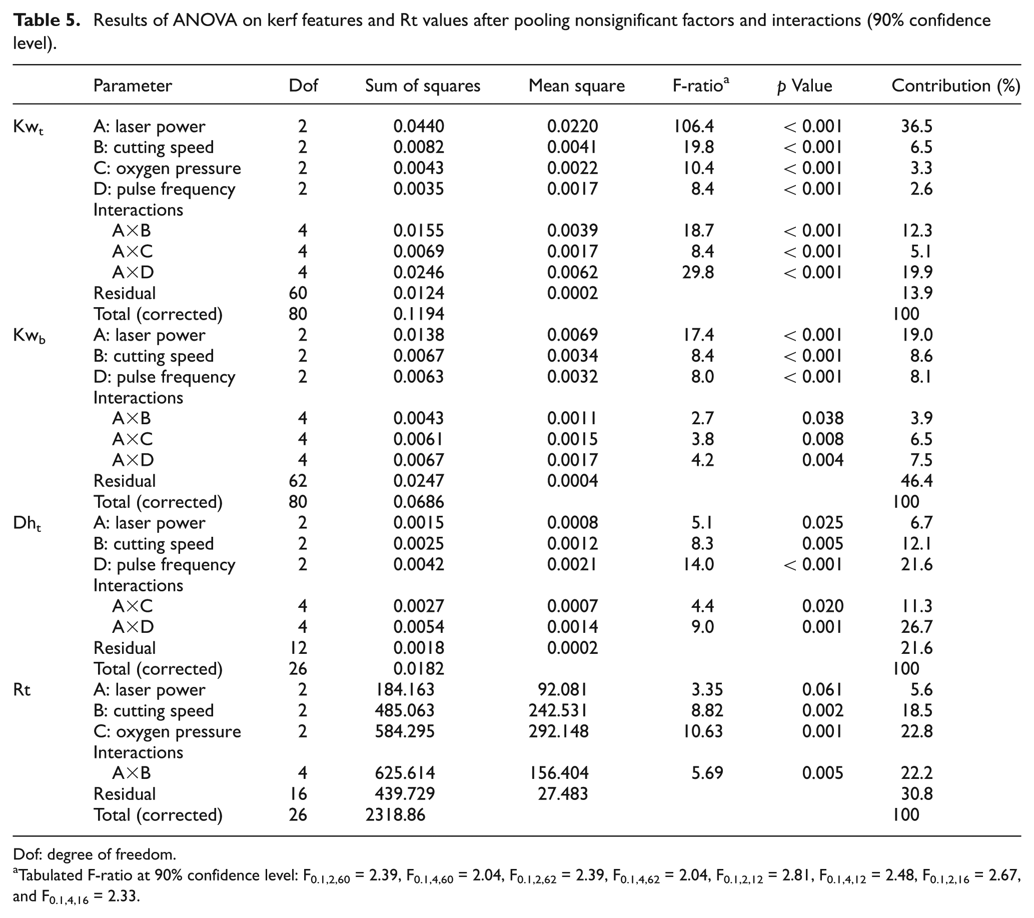
Dof: degree of freedom.

a

Tabulated F-ratio at 90% confidence level: F_0.1,2,60 = 2.39, F_0.1,4,60 = 2.04, F_0.1,2,62 = 2.39, F_0.1,4,62 = 2.04, F_0.1,2,12 = 2.81, F_0.1,4,12 = 2.48, F_0.1,2,16 = 2.67, and F_0.1,4,16 = 2.33.

Table 6.

Results of ANOVA on S/N_S ratios after pooling nonsignificant factors and interactions (90% confidence level).

	Parameter	Dof	Sum of squares	Mean square	F-ratio a	p Value	Contribution (%)
Kwt	A: laser power	2	6.1032	3.0516	41.84	<0.001	39.2
	B: cutting speed	2	0.9907	0.4953	6.79	0.029	5.6
	C: oxygen pressure	2	0.5312	0.2656	3.64	0.092	2.5
	D: pulse frequency	2	0.5982	0.2991	4.1	0.075	3.0
	Interactions
	A×B	4	1.9116	0.4779	6.55	0.022	10.6
	A×C	4	0.9747	0.2437	3.34	0.091	4.5
	A×D	4	3.6692	0.9173	12.58	0.004	22.2
	Residual	6	0.4376	0.0729			12.5
	Total (corrected)	26	15.2163				100
Kwb	A: laser power	2	5.5431	2.7715	6.2	0.008	23.1
	B: cutting speed	2	2.6931	1.3465	3.01	0.072	9.0
	D: pulse frequency	2	2.9117	1.4558	3.26	0.060	10.0
	Residual	20	8.9416	0.4471			57.9
	Total (corrected)	26	20.0895				100
Dht	B: cutting speed	2	111.755	55.877	10.3	0.002	17.0
	D: pulse frequency	2	134.692	67.346	12.4	<0.001	20.8
	Interactions
	A×C	4	78.835	19.709	3.6	0.032	9.6
	A×D	4	192.8576	48.214	8.9	<0.001	28.8
	Residual	14	76.2647	5.4474			23.8
	Total (corrected)	26	594.404				100
Rt	A: laser power	2	14.767	7.384	2.66	0.100	4.0
	B: cutting speed	2	43.547	21.774	7.84	0.004	16.6
	C: oxygen pressure	2	62.950	31.475	11.34	<0.001	25.1
	Interactions
	A×B	4	62.685	31.342	5.65	0.005	22.6
	Residual	16	44.412	2.776			31.6
	Total (corrected)	26	228.362				100

a

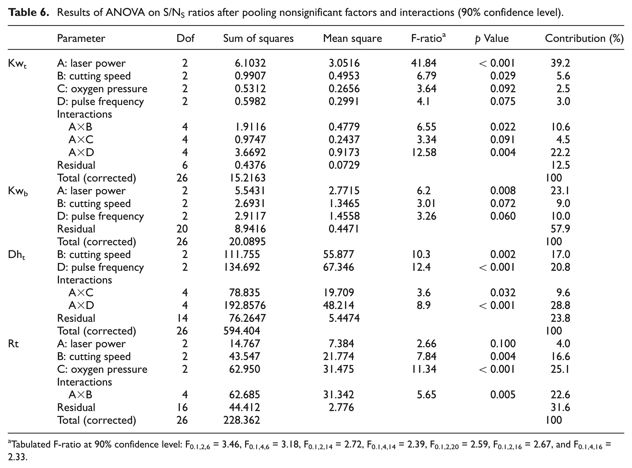
Tabulated F-ratio at 90% confidence level: F_0.1,2,6 = 3.46, F_0.1,4,6 = 3.18, F_0.1,2,14 = 2.72, F_0.1,4,14 = 2.39, F_0.1,2,20 = 2.59, F_0.1,2,16 = 2.67, and F_0.1,4,16 = 2.33.

The ANOVA on the raw data shows that all the process parameters are statistically significant (at a 90% confidence level) for the top kerf width, also including the interaction between the laser power and the other control factors. Similar considerations can be made for S/N_S ratios. The laser power is the main contributor to the top kerf width, in terms of the average effect and the S/N_S ratio approaches (36.5 and 39.2%, respectively), and this is followed by the interaction between the laser power and the pulse frequency (19.9 and 22.2, respectively). The overall contribution of the other parameters is limited to about 30%.

All the control factors, except the oxygen pressure, and interactions are also statistically significant for the bottom kerf width. However, the interaction factors are not significant when the S/N_S values are considered. The laser power contributes most to the bottom kerf width (19.0% and 23.1% for the raw and the S/N_S data, respectively); nevertheless, the contribution of the residual is quite high, around 50%.

The laser power, cutting speed, and pulse frequency of the laser beam, as well as the interaction of the laser power with oxygen pressure and pulse frequency, are significant for the top kerf deviation. Similar significant factors have been found for the S/N_S values, except for the laser power. The pulse frequency and its interaction with the laser power contribute to 50% of the top kerf deviation; similar trends can be detected for the S/N_S ratios, the residual being limited to about 21%–24%.

The laser power, oxygen pressure, cutting speed, and the interaction between the laser power and cutting speed are the most significant factors for Rt. It can be noted that the contribution of the laser power is less of the other control factors.

Effect of the significant cutting parameters

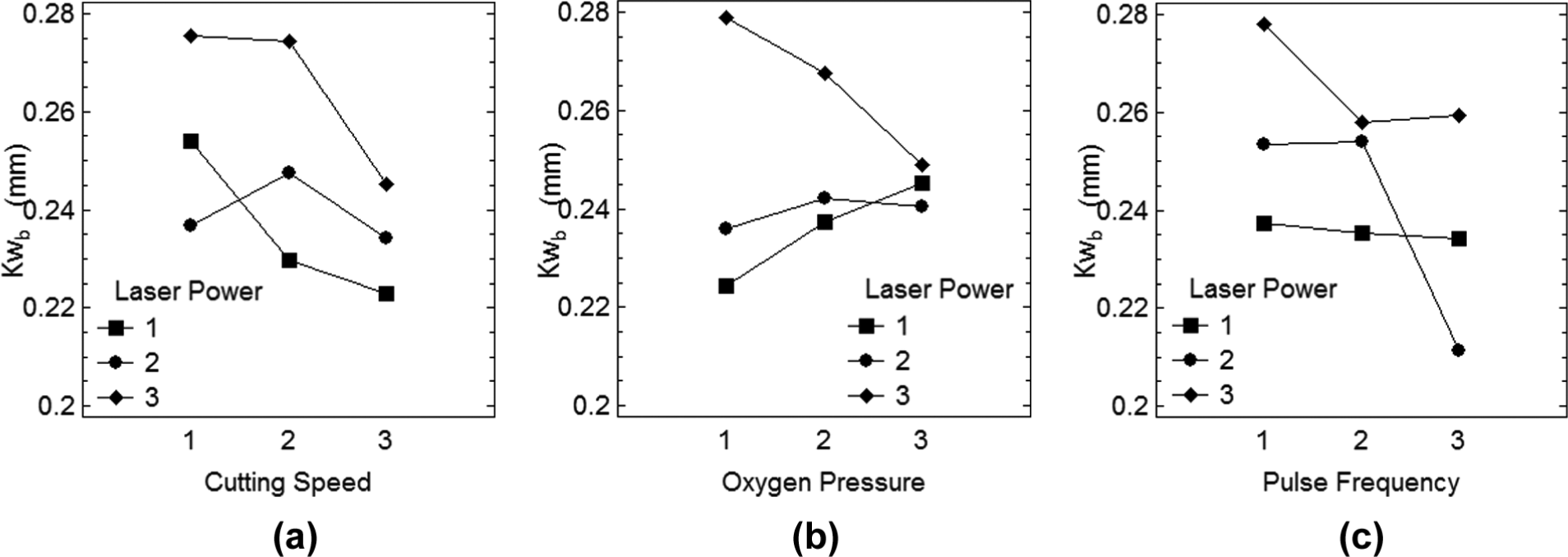
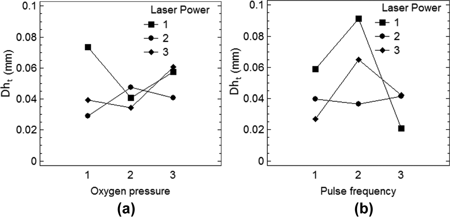
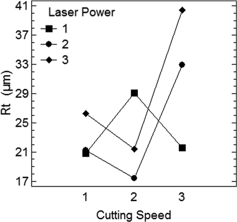
The mean responses of the kerf features and roughness values are calculated to evaluate the effect of the significant process parameters for each of the three-level factor. The ensuing response graphs are depicted in Figure 5 (the x-axis indicates the three levels of each process parameter, while the y-axis indicates either the kerf feature or Rt response), in terms of raw data and S/N_S ratios. The means of the raw data and S/N_S ratios are calculated at levels 1–3 by averaging the kerf features and roughness values of the experimental trials 1–9, 10–18, and 19–27, respectively. The significant process parameters that exhibit large differences in the Kw_t, Kw_b, Dh_t, and Rt values indicate a notable effect on these features as their level is changed. Regardless of the response graphs, the nonstatistically significant process parameters do not have any discernible effects on kerf features and roughness.

Figure 5.

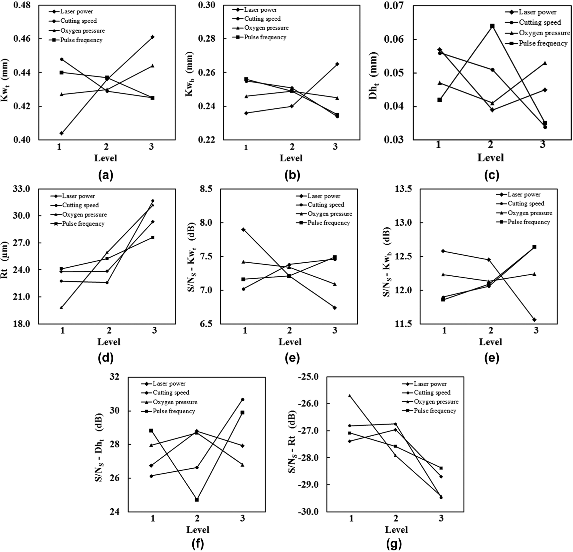
Response graph for (a, e) top kerf width, (b, f) bottom kerf width, (c, g) top kerf deviation, and (d, h) roughness: (a–d) raw data and (e–h) S/N_S ratios.

The laser power shows the largest variation in level for the Kw_t; therefore, it is the main factor that affects this kerf feature. In particular, the Kw_t enlarges with a quasi-linear trend with the laser power, ranging from about 0.40 to 0.46 mm (Figure 5(a)). The laser power is also the most important parameter affecting the Kw_b (Figure 5(b)). In this case, the Kw_b becomes significantly larger only when the maximum laser power is used, varying of about 0.03 mm from levels 1 to 3 of the laser power. The effect of the laser power on the kerf width is obvious: as the laser power increases, the amount of thermal energy supplied per unit time to the sheet increases, and, in turn, the kerf widens. As expected, with increasing laser power, the top kerf width, where the laser beam first hits the sheet, widens more than the bottom one (0.06 vs 0.03 mm). Moreover, greater kerf tapers (the difference between the top and bottom kerf width) occur when the supplied thermal energy reduces. The influence of the laser power on the Dh_t and Rt is less evident. At most, it can be inferred that the highest values of Rt are basically obtained from high laser power values. In these cases, more thermal energy is supplied to the workpiece, and sideways burning enhances the peak-to-valley distance of the striations on the cut surfaces.

The interaction between the laser beam and the metal sheet reduces as the cutting speed increases; in this condition, narrower kerfs are obtained (Figure 5(a) and (b)). This reduction in kerf width has a similar trend for both the sides of the sheets, with the average values of the Kw_t and Kw_b that decrease of about 0.02 mm from levels 1 to 3 of the cutting speed. The total height of the roughness profile increases with the cutting speed. To explain this result, two factors that might affect the roughness of the cut surfaces have to be considered: ³² (1) the cut front geometry becomes curved or kinked at high cutting speeds and (2) the melt thickness on the cut front increases with cutting speed. In the former case, the curve or kinked cut front profile causes a notable directional change of the molten material from the top to the bottom of cut the surface, thereby originating a melt deceleration and a subsequent turbulence, which leads to an increase of surface roughness. In the latter case, higher cutting speeds promote an increase of the melt flow in the cross section of the sheet and hence a more intensive melt turbulence, which badly affects surface roughness.

As well known, the oxygen gas exerts two main effects during the laser cutting process; first, the oxygen gas reacts exothermically with the molten metal, thus enhancing the thermal energy that is available for the cutting; second, it ejects the oxidized melt from the kerf. Therefore, more molten material can be removed from the cutting zone as the oxygen pressure increases, and wider kerfs can be obtained. In this work, however, the oxygen pressure does not seem to be a relevant factor for kerf width; in fact, it has only a limited effect on the top kerf width (Figure 5(a)), and it is not statistically significant for the bottom one (Figure 5(b), Tables 5 and 6). To explain this, it is assumed that the extent of the oxidation reaction is limited by the low laser power used in the experimental tests (up to 315 W). This means that for the examined range of the laser power, an increase in oxygen pressure above 2 bar does not enhance oxidation of the molten metal. Therefore, an oxygen pressure above this level is excessive for metal oxidation and may only be necessary to remove the molten oxide from the cutting zone. Higher laser power and lower oxygen pressure values would be required to reveal a more significant effect of the oxygen pressure on kerf width, as previously reported by Yilbas et al. ³³ Moreover, the assist gas presumably reached a sonic velocity as the oxygen pressure was above 2 bar, so any further increase in pressure only decreased the pressure drop in the nozzle without increasing the jet velocity significantly. ³⁴ This might justify the slight increase of the top kerf width shown in Figure 5(a) as oxygen pressure increases from 2 to 4 bar. The oxygen pressure exhibits the most important effect on the peak-to-valley distance of the striations; in particular, the risk of turbulence within the molten metal increases as the oxygen pressure increases, badly affecting the roughness profile. Overall, Rt increases from about 19 to 32 µm (Figure 5(d)).

The pulse frequency of the laser beam appears to decrease kerf width in the both sides of the TWIP steel sheets. As the pulse frequency of the laser beam, and hence the overlapping of laser pulses, increases, the energy of each laser input decreases, thus leading to less molten material and to reduced kerf widths (Figure 5(a) and (b)). Generally, the shorter distance between two laser pulses should reduce kerf deviation; ³⁵ however, this does not occur in this work. Indeed, the corresponding response graph exhibits an irregular trend from levels 1 to 3 of the control factor (Figure 5(c)): average Dh_t first increases from about 0.04 to 0.065 mm and then decreases to 0.035 mm. The shorter distance between two laser pulses should also reduce roughness overall, ³⁵ but the pulse frequency of the laser beam is not statistically significant on Rt (Tables 5 and 6). Probably, the durations of the examined laser pulses were too short (0.5, 0.67, and 1 ms) to detect any significant effects on roughness. Interaction plots of the significant interactions between laser power and the other control factors are shown in Figures 6–8.

Figure 6.

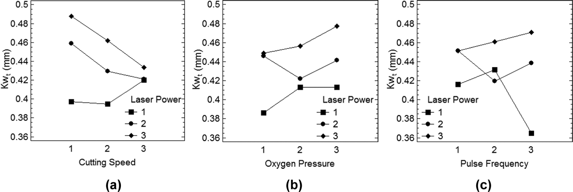
Plots of the interactions (a) A×B, (b) A×C, and (c) A×D about top kerf width.

Figure 7.

Plots of the interactions (a) A×B, (b) A×C, and (c) A×D about bottom kerf width.

Figure 8.

Plots of the interactions (a) A×C and (b) A×D about top kerf deviation.

The interaction plots mainly confirm the effects of the significant parameters mentioned for the response graphs. Therefore, the largest kerf widths are obtained when more thermal energy is supplied to the workpiece per unit time, primarily due to low cutting speed and high laser power (Figures 6(a) and 7(a)). It should also be noted that the top kerf width reduces more as cutting speed increases, for high laser power (levels 2 and 3); this is because the oxidation reaction is more intensive for high laser power, and hence, it is more sensitive to the variation of the cutting speed. This trend can also be seen for the bottom kerf width (Figure 7(a)).

Interaction plot of Figure 6(b) shows that oxygen pressure has about the same effect, regardless of the laser power employed: the top kerf width tends to increase of about 0.02 mm with increasing laser power. A similar effect can also be detected for the bottom kerf width (Figure 7(b)), even though the Kw_b decreases with increasing oxygen pressure as the highest laser power is used. In this case, the dross attachment is absent, thereby reducing the extent of the bottom kerf width (see the classes of cuts in Table 4). The interaction between the laser power and the oxygen pressure has nearly the same effect on kerf deviation (Figure 8(a)), with a small increase in the Dh_t probably due to the slightly more intensive oxidation reaction and turbulence of the assist gas.

The interaction plots concerning the interaction between the laser power and the pulse frequency of the laser beam appear quite irregular (Figures 6(c), 7(c), and 8(b)), so this interaction does not exhibit a clear effect on all the examined kerf features.

The interaction plot of Figure 9 emphasizes that the peak-to-valley distance of the striations is more affected by the highest cutting speed, especially as the laser power at levels 2 or 3 is employed. In particular, this trend seems to assess that the increase of Rt mainly depends on the melt thickness on the cut front rather than on the cut front geometry (curved or kinked) at high cutting speeds. The average response graphs and significant interaction plots of S/N_S ratios have been omitted in the text, as the same comments mentioned for the average effect data can be made.

Figure 9.

Plot of the interactions A×B about total height of the roughness profile of the cut surfaces.

Estimation of the optimal laser cutting process parameters

The estimated mean values of the kerf and roughness responses at the optimal condition, m_opt, are computed by the Taguchi method (see section “Taguchi method for process parameters design”). The significant process parameters and interactions have already been identified from the ANOVA results (Tables 5 and 6), while their optimal settings are those that minimize the mean values of the Kw_t, Kw_b, Dh_t, and Rt. The optimal settings of the process parameters are obtained by the minimum mean output responses listed in Table 7. Regardless of the statistical significance, the following optimal settings of the factor levels can be identified for the Kw_t, Kw_b, Dh_t, and Rt, respectively: A₁B₃C₁D₃, A₁B₃C₃D₃, A₂B₃C₂D₃, and A₁B₂C₁D₁. These optimal factor levels are the same for the S/N_S ratios.

Table 7.

Mean kerf features and roughness values for each level of the control factors (raw data and S/N_S ratios).

Response	Factor	Raw data			S/NS ratio (dB)
		Level 1	Level 2	Level 3	Level 1	Level 2	Level 3
Kwt (mm)	Laser power	0.404opt	0.436	0.461	7.90opt	7.21	6.74
	Cutting speed	0.448	0.429	0.425opt	7.02	7.38	7.46opt
	Oxygen pressure	0.427opt	0.430	0.444	7.42opt	7.34	7.09
	Pulse frequency	0.440	0.437	0.425opt	7.16	7.21	7.49opt
Kwb (mm)	Laser power	0.236opt	0.240	0.265	12.58opt	12.45	11.56
	Cutting speed	0.255	0.251	0.234opt	11.90	12.06	12.64opt
	Oxygen pressure	0.246	0.249	0.245opt	12.23	12.13	12.24opt
	Pulse frequency	0.256	0.249	0.235opt	11.86	12.09	12.64opt
Dht (mm)	Laser power	0.057	0.039opt	0.045	26.76	28.80opt	27.93
	Cutting speed	0.056	0.051	0.034opt	26.15	26.65	30.69opt
	Oxygen pressure	0.047	0.041opt	0.053	27.97	28.70opt	26.81
	Pulse frequency	0.042	0.064	0.035opt	28.84	24.73	29.91opt
Rt (µm)	Laser power	23.80opt	23.85	29.37	−27.38	−26.96opt	−28.70
	Cutting speed	22.75	22.60opt	31.67	−26.82	−26.75opt	−29.48
	Oxygen pressure	19.84opt	25.96	31.22	−25.71opt	−27.91	−29.42
	Pulse frequency	24.13opt	25.27	27.62	−27.09opt	−27.58	−28.37

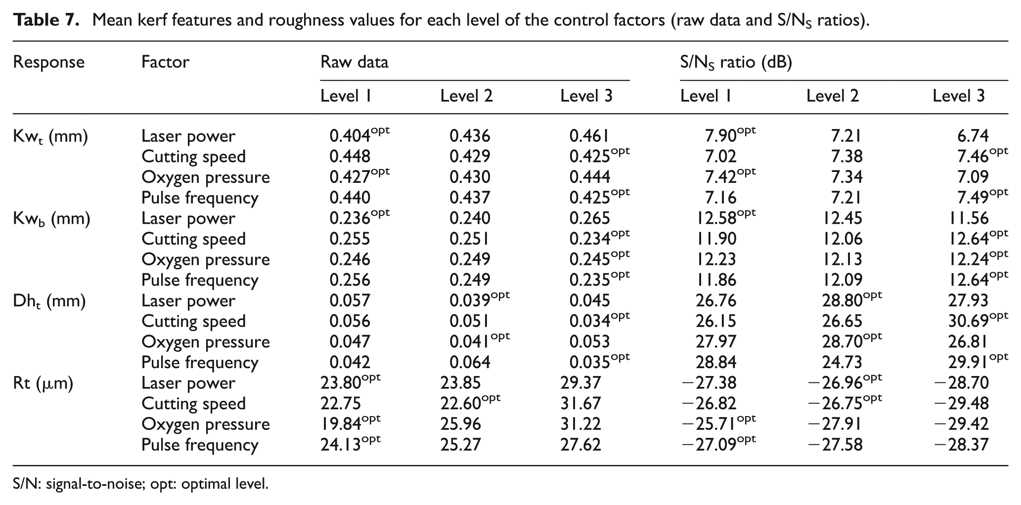
S/N: signal-to-noise; opt: optimal level.

As far as interactions are concerned, based on the average effect of the process parameters, the A₁×D₃ interaction is considered in the calculation of the optimal Kw_t value, while the A₂×D₃, A₁×D₃, and A₂×B₂ interactions are considered to calculate the optimal Kw_b, Dh_t, and Rt values, respectively. It can be seen from Table 4 that the A₁ and D₃ factor levels are included in trials 3, 5, and 7; the A₂ and D₃ factor levels are in trials 11, 13, and 18, while the A₂ and B₂ factor levels are in trials 13, 14, and 15. The above-mentioned interactions give an average contribution of 0.365, 0.211, 0.021 mm, and 17.39 µm in the calculation of the optimal Kw_t, Kw_b, Dh_t, and Rt values, respectively. Finally, the optimal estimated mean is calculated taking into account at first the contribution of the most significant interaction and then those of the remaining significant control factors (excluding the process parameters already considered in the interaction), as follows

$$\begin{array}{l}\multicolumn{1}{c}{{\text{m}}_{\text{K}{\text{w}}_{\text{t}}-\text{opt}}={({\text{A}}_1\times {\text{D}}_3+{\text{B}}_3+{\text{C}}_1-2·\stackrel{·}{\text{T}})}_{\text{K}{\text{w}}_{\text{t}}}}\\ =0.365+0.425+0.427-2·0.434\\ =0.349\text{mm}\end{array}$$

$$\begin{array}{c}\multicolumn{1}{c}{{\text{m}}_{\text{K}{\text{w}}_{\text{b}}-\text{opt}}={({\text{A}}_2\times {\text{D}}_3+{\text{B}}_3+{\text{C}}_3-2·\stackrel{·}{\text{T}})}_{\text{K}{\text{w}}_{\text{b}}}}\\ =0.211+0.234+0.245-2·0.247\hfill \\ =0.196\text{mm}\hfill \end{array}$$

$$\begin{array}{c}\multicolumn{1}{c}{{\text{m}}_{\text{D}{\text{h}}_{\text{t}}-\text{opt}}={({\text{A}}_1\times {\text{D}}_3+{\text{B}}_3-\stackrel{·}{\text{T}})}_{\text{D}{\text{h}}_{\text{t}}}}\\ =0.021+0.034-0.047=0.008\text{mm}\hfill \end{array}$$

$$\begin{array}{c}\multicolumn{1}{c}{{\text{m}}_{\text{Rt}-\text{opt}}={({\text{A}}_2\times {\text{B}}_2+{\text{C}}_1-\stackrel{·}{\text{T}})}_{\text{Rt}}}\\ =17.39+19.84-25.67=11.56\mu \text{m}\hfill \end{array}$$

where ${\stackrel{·}{\text{T}}}_{\text{K}{\text{w}}_{\text{t}}}$ , ${\stackrel{·}{\text{T}}}_{\text{K}{\text{w}}_{\text{b}}}$ , ${\stackrel{·}{\text{T}}}_{\text{D}{\text{h}}_{\text{t}}}$ , and ${\stackrel{·}{\text{T}}}_{\text{Rt}}$ are given in Table 4.

Based on S/N_S, the A₁×D₃ interaction contributes to the calculation of the optimal Kw_t and Dh_t values, while the A₂×B₂ interaction contributes for computing the optimal Rt value. From Table 4, A₁ and D₃ factor levels are included in trials 3, 5, and 7, while A₃ and D₁ factor levels are included in trials 13, 14, and 15. The above-mentioned interactions give an average contribution of 8.76, 33.60, and −27.68 dB in the calculation of the Kw_t, Dh_t, and Rt values, respectively. The optimal estimated means for the kerf features and roughness are then calculated as follows

$$\begin{array}{l}\multicolumn{1}{c}{{\text{m}}_{\text{S}/{\text{N}}_{\text{S}}-\text{K}{\text{w}}_{\text{t}}-\text{opt}}={({\text{A}}_1\times {\text{D}}_3+{\text{B}}_3+{\text{C}}_1-2·\stackrel{·}{\text{T}})}_{\text{S}/{\text{N}}_{\text{S}}-\text{K}{\text{w}}_{\text{t}}}}\\ =8.76+7.46+7.42-2·7.28\\ =9.08\text{dB}\end{array}$$

$$\begin{array}{c}\multicolumn{1}{c}{{\text{m}}_{\text{S}/{\text{N}}_{\text{S}}-\text{K}{\text{w}}_{\text{b}}-\text{opt}}={({\text{A}}_1+{\text{B}}_3+{\text{D}}_3-2·\stackrel{·}{\text{T}})}_{\text{S}/{\text{N}}_{\text{S}}-\text{K}{\text{w}}_{\text{b}}}}\\ =12.58+12.64+12.64-2·12.20\hfill \\ =13.46\text{dB}\hfill \end{array}$$

$$\begin{array}{cc}\multicolumn{1}{c}{{\text{m}}_{\text{S}/{\text{N}}_{\text{S}}-\text{D}{\text{h}}_{\text{t}}-\text{opt}}}& ={({\text{A}}_1\times {\text{D}}_3+{\text{B}}_3-\stackrel{·}{\text{T}})}_{\text{S}/{\text{N}}_{\text{S}}-\text{D}{\text{h}}_{\text{t}}}\hfill \\ =33.60+30.69-27.83=36.46\text{dB}\hfill \end{array}$$

$$\begin{array}{cc}\multicolumn{1}{c}{{\text{m}}_{\text{S}/{\text{N}}_{\text{s}}-\text{Rt}-\text{opt}}}& ={({\text{A}}_2\times {\text{B}}_2+{\text{C}}_1-\stackrel{·}{\text{T}})}_{\text{S}/{\text{N}}_{\text{S}}-\text{Rt}}\hfill \\ =-24.79-25.71+27.68\hfill \\ =-22.82\text{dB}\hfill \end{array}$$

where ${\stackrel{·}{\text{T}}}_{\text{S}/{\text{N}}_{\text{S}}-\text{K}{\text{w}}_{\text{t}}}$ , ${\stackrel{·}{\text{T}}}_{\text{S}/{\text{N}}_{\text{S}}-\text{K}{\text{w}}_{\text{b}}}$ , ${\stackrel{·}{\text{T}}}_{\text{S}/{\text{N}}_{\text{S}}-\text{D}{\text{h}}_{\text{t}}}$ , and ${\stackrel{·}{\text{T}}}_{\text{S}/{\text{N}}_{\text{S}}-{\text{R}}_{\text{t}}}$ are given in Table 4. From these data, inverting equation (2) and then applying equation (7), the following expected responses are obtained

$${\text{Y}}_{\text{exp}-\text{K}{\text{w}}_{\text{t}}}=0.352\text{mm}$$

$${\text{Y}}_{\text{exp}-\text{K}{\text{w}}_{\text{b}}}=0.212\text{mm}$$

$${\text{Y}}_{\text{exp}-\text{D}{\text{h}}_{\text{t}}}=0.015\text{mm}$$

$${\text{Y}}_{\text{exp}-\text{Rt}}=13.84\mu \text{m}$$

The 90% CIs of the predicted optimal kerf features and roughness are calculated using equation (12). For the Kw_t interval, F_0.1,1,60, N, and R are 2.791, 81, and 3, respectively. The total dof associated with the estimated optimal mean is 8 (dof of A×D, B, and C parameters), and the error variance Ve is 0.0002. For the Kw_b interval, F_0.1,1,62, N, and R are 2.788, 81, and 3, respectively. The total dof associated with the estimated optimal mean is 8 (dof of A×D, B, and C parameters), and the error variance Ve is 0.0004. For the Dh_t interval, F_0.1,1,12, N, and R are 3.176, 27, and 3, respectively. The total dof associated with the estimated optimal mean is 6 (dof of A×D and B parameters), and the error variance Ve is 0.0002. For the Rt interval, F_0.1,1,16, N, and R are 3.048, 27, and 1, respectively. The total dof associated with the estimated optimal mean is 6 (dof of A×D and C parameters), and the error variance Ve is 20.060. With these data, the 90% CIs of the predicted optimal kerf features and roughness are

$$0.333\text{mm}<\text{K}{\text{w}}_{\text{t}}<0.365\text{mm}(\text{CI}=0.016\text{mm})$$

$$0.174\text{mm}<\text{K}{\text{w}}_{\text{b}}<0.218\text{mm}(\text{CI}=0.022\text{mm})$$

$$0\text{mm}<\text{D}{\text{h}}_{\text{t}}<0.027\text{mm}(\text{CI}=0.019\text{mm})$$

$$1.29\mu \text{m}<\text{Rt}<21.81\mu \text{m}(\text{CI}=10.27\mu \text{m})$$

Based on the S/N_S ratio approach, F_0.1,1,6, N, and R are 3.776, 27, and 3 for the Kw_t interval, respectively. The total dof associated with the estimated optimal mean is 8 (dof of A×D, B, and C parameters), and the error variance Ve is 0.0729. For the Kw_b interval, F_0.1,1,20, N, and R are 2.975, 27, and 3, respectively. The total dof associated with the estimated optimal mean is 6 (including A, B, and D parameters), and the error variance Ve is 0.4471. For the Dh_t interval, F_0.1,1,14, N, and R are 3.102, 27, and 3, respectively. The total dof associated with the estimated optimal mean is 6 (including A×D and B parameters), and the error variance Ve is 5.447. For the Rt interval, F_0.1,1,16, N, and R are 3.048, 27, and 1, respectively. The total dof associated with the estimated optimal mean is 6 (including A×D and C parameters), and the error variance Ve is 2.0840. With these data, the 90% CIs of the predicted optimal kerf features and roughness are

$$8.652\text{dB}<\text{K}{\text{w}}_{\text{t}}<9.508\text{dB}(\text{CI}=0.428\text{dB})$$

$$12.572\text{dB}<\text{K}{\text{w}}_{\text{b}}<14.348\text{dB}(\text{CI}=0.888\text{dB})$$

$$33.296\text{dB}<\text{D}{\text{h}}_{\text{t}}<39.624\text{dB}(\text{CI}=3.164\text{dB})$$

$$-26.084\text{dB}<\text{Rt}<-19.556\text{dB}(\text{CI}=3.264\text{dB})$$

Confirmation experiments

Three confirmation experimental tests were carried out using the laser cutting process parameters at the optimal levels to validate the predicted optimal kerf and roughness responses. The nonstatistically significant factors could be set at any desired level because their effect on the cut quality was negligible. In this case, the level of each insignificant factor had been set according to the optimal value given in Table 7. Both the average effect and the S/N_S ratio approaches gave A₁B₃C₁D₃ and A₁B₃C₂D₃ as the optimal combinations for Kw_t and Dh_t, respectively, while the combinations A₂B₃C₃D₃ and A₁B₃C₃D₃ resulted for the Kw_b in terms of average effect and S/N_S ratio, respectively. As far as Rt was concerned, the optimal combinations were A₁B₂C₁D₁ and A₂B₂C₁D₁ from raw data and S/N ratios, respectively.

After the confirmation tests, the average Kw_t, Kw_b, Dh_t, and Rt values were found to be 0.347, 0.202, 0.018 mm, and 17.6 µm, respectively, which are 9.193, 13.893, 34.895, and −24.91 dB in terms of S/N_S ratio, respectively. These results are within the 90% CIs of the predicted optimal kerf and roughness responses.

Summary

A design of experiments based on the Taguchi approach has been adopted to evaluate the effect of laser process parameters on the cut quality of 1.5-mm TWIP steel sheets. Laser process parameters were laser power, cutting speed, oxygen pressure, and pulse frequency of the CO₂ laser beam. Cut quality was evaluated in terms of top kerf width, bottom kerf width, kerf deviation, striation pattern, peak-to-valley distance of striations, and dross attachment. An L27(3¹³) orthogonal array has been used to design the experiments and predict the optimal process parameter combinations that allow the best quality of the cut edges to be obtained.

Low laser power and cutting speed promote the formation of quite regular striation patterns with short peak-to-valley distances, while increasing the cutting speed, the striations tend to curve and the cut surfaces appear more irregular, thereby exhibiting higher Rt values. Sideways burning seems to be the main cause for the formation of striation patterns. The dross attachment, evaluated by three classes of cuts, is more pronounced when high laser power and low cutting speed are employed. Overall, there is no clear relationship among kerf width, roughness of the cut surfaces, and dross attachment.

According to the ANOVA results, the laser power is the process parameter that has the most effect on kerf width. The top and bottom kerf width increase with increasing laser power. On the contrary, the oxygen pressure has a limited effect on all the examined kerf features. Presumably, the oxygen pressure above 2 bar is excessive for metal oxidation and may only be necessary to remove the molten oxide from the cutting zone. A pressure drop in the nozzle of the assist gas, at sonic velocity, might have limited the increase of the top kerf width (about 0.02 mm) at increasing oxygen pressure. Overall, higher laser power and lower oxygen pressure values would be required to reveal a more significant effect of the oxygen pressure on kerf width.

The turbulence within the molten metal increases as the oxygen pressure increases, badly affecting the roughness profile. Moreover, the total height of the roughness profile increases as the cutting speed increases; this is mainly due to the increase in melt thickness on the cut front, as suggested by the corresponding interaction plot.

As the pulse frequency of the laser beam, and hence the overlapping of laser pulses, increases, the energy of each laser input decreases, thus leading to reduced kerf widths and kerf deviation. However, this process parameter does not affect Rt; probably, the durations of the examined laser pulses were too short.

The optimal parameter combinations for the examined kerf features are the same in terms of the average effect and the S/N_S ratio, but different for Kw_b and Rt. They are A₁B₃C₁D₃ and A₁B₃C₂D₃ for Kw_t and Dh_t; A₂B₃C₃D₃ and A₁B₃C₃D₃ for Kw_b; and A₁B₂C₁D₁ and A₂B₂C₁D₁ for Rt. Confirmation tests have shown that an optimal combination of the process parameters allows the best cut quality to be obtained within the predicted CIs.