Prediction of loading path for tube hydroforming with radial crushing by combining genetic algorithm and bisection method

Abstract

Tube hydroforming with radial crushing is a new tube hydroforming process to manufacture very long components with complex cross sections. A loading path is generally considered a major factor that greatly affects the formability of a component by tube hydroforming. In this study, the tube hydroforming with radial crushing process of a square cross-sectional component was investigated by using the finite element method, and a method to predict the optimal loading path for the tube hydroforming with radial crushing process was developed from the finite element simulation. A multi-object function was first built in terms of the die-filling ability, cross-sectional symmetry, and wall thickness uniformity. Subsequently, a multi-strategy approach, characterized by a genetic algorithm and the bisection method, was developed to predict the optimal loading path. The effectiveness of the prediction method was verified by comparing the formability of components deformed under the optimal and conventional loading paths. Furthermore, the developed multi-strategy approach was demonstrated to have high efficiency when the total calculation times for the multi-strategy approach and for genetic algorithm alone were compared.

Keywords

Tube hydroforming loading path genetic algorithm bisection method finite element method

Introduction

The process of tube hydroforming (THF) is one of the near net shape techniques for producing tubular components, which are widely used in many fields including the automotive, aviation, aerospace, and household appliance industries. During the THF process, axial feeding is generally applied to the tube ends to drive the material flowing toward the bulging zone and avoid bursting failure. However, axial feeding is also thought to contribute to wrinkling and buckling failure. To resolve these issues, Morphy¹ proposed a novel THF process without axial feeding, namely, THF with radial crushing (THFRC), which is reportedly an efficient method to deform very long components with complex cross sections.

The formability of a component by THFRC is greatly affected by the loading path, as is the case in the conventional THF process. Because an improper loading path can lead to forming failures such as bursting, wrinkling, or buckling, a proper or optimal loading path should be designed to improve the formability and avoid any failure of the deformed component. The typical methods used thus far to predict loading paths for THF are summarized as follows:

Theoretical analysis methods based on theories of plasticity have been used to analyze the forming limit of the component and predict the tendency of the optimal loading path to vary.^2,3 However, the applicability of these methods is limited because of the excessive number of assumptions and the complex theoretical derivations to build the model.

The trial-and-error method in combination with experimental analysis or the finite element method (FEM) has been implemented to search the optimal loading path for given components.^4,5 Although this method is easy to use in the absence of complex theoretical derivations, it is time-consuming and costly due to its case-by-case nature in accordance with various components. Moreover, there is no guarantee of finding the optimal loading path by using this method.

The gradient-based optimization method has been used to search for the optimal loading conditions, such as for punch force in sheet forming and hydraulic pressure in THF.^6–8 This method is highly efficient owing to its ability to adjust the searching direction during the search process to keep it parallel to the steepest gradient direction at each searching step. By this method, the globality of the searching result is considered to rely on selection of the initial point of the searching process. If the initial point is estimated inappropriately, the local rather than global optimum is likely to be obtained.

Methods that mimic the process of natural evolution, such as genetic algorithms (GA) and annealing algorithms, have been carried out to predict a multi-object optimal loading path for the THF process.^8,9 The optimal loading path can be obtained by implementing these evolution-based algorithms because of their powerful global searching capacity. Nonetheless, the prediction process is usually time-consuming owing to the requirement of large iterations for high-precision results.

Human-simulated intelligent control (HSIC) methods such as neural network, fuzzy logic control, and adaptive simulation methods have been utilized to predict the optimal loading path.^4,10,11 HSIC methods save time because an optimal loading path can be obtained with only one instead of many iterative operations. However, HSIC controllers are built on the basis of large training samples, and their controlling accuracy depends on the perfection of their expert system. Developing a powerful HSIC controller with limited time is difficult.

Complex methods that combine two or more types of optimization strategies have been built to search for the optimal loading path of the THF process,^12–15 with the aim of saving time and achieving ease of use. These methods, owing to their advantage of combining the merits of the building block strategies, are used effectively to search for the optimal solution with a high degree of efficiency.

Predicting the proper loading path for the THF process is one of the greatest challenges in the field. In this study, the forming behavior of a square cross-sectional component in THFRC was investigated by using the FEM, and a complex method of predicting the optimal loading path, involving the evaluation of formability and construction of a prediction strategy, was developed. A multi-object function was constructed on the basis of the weighted order of the formability indicators, after which a multi-strategy approach that combined GA and the bisection method (BM) was proposed for predicting the optimal loading path. The effectiveness of the method was demonstrated by comparing the formability of the components deformed under the optimal and conventional loading paths. The high efficiency of the multi-strategy approach was verified by comparing its total calculation time with that of GA alone.

Brief introduction of THFRC

The THFRC process has been investigated and applied previously.^16–18 This process is mainly composed of three stages: a free hydraulic bulging (FHB) stage, a combined forming stage, and a calibrating stage (Figure 1). In the FHB stage, a round tubular blank with an initial outside diameter (OD) of D₀ is freely expanded by the mere hydraulic pressure P into a larger one with an OD of D₁. The expansion is stopped before the outer surface of the tube contacts the upper and the lower dies (Figure 1(b)). Subsequently, in the combined forming stage (Figure 1(c)), the tube is crushed into one with a square cross section by both the radial force from the closing of the dies and the hydraulic pressure P, until the dies close completely. Finally, a component with a square cross section is obtained in the following calibrating stage (Figure 1(d)).

Figure 1.

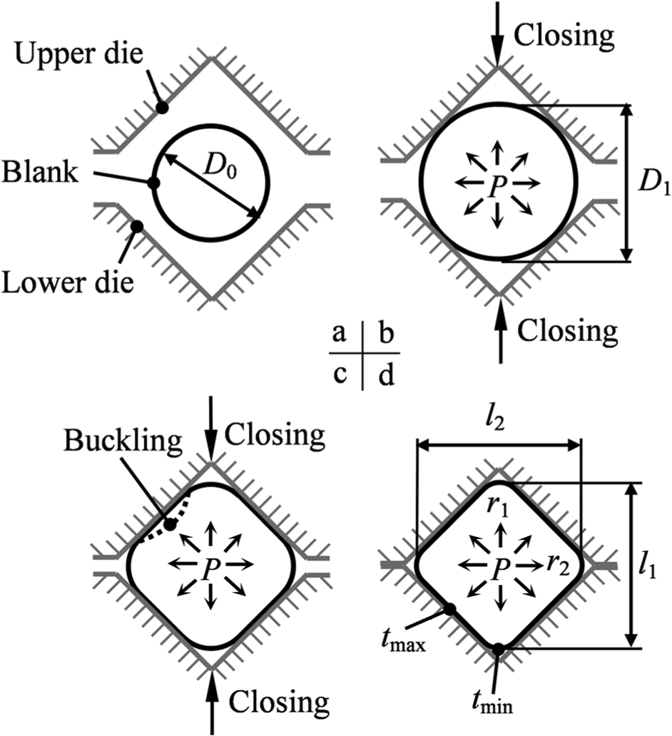
Schematic diagram of tube hydroforming with radial crushing (THFRC) process (cross-sectional view): (a) blank locating, (b) free hydraulic bulging (FHB), (c) combined forming, and (d) final calibrating.

The formability of the component by THFRC can be evaluated in terms of the die-filling ability (the fillet radii r₁ and r₂), cross-sectional symmetry (the difference in diagonal lengths, Δl=l₂−l₁), and wall thickness uniformity (the difference in wall thicknesses, Δt= t_max−t_min), as illustrated in Figure 1. A component with good formability is characterized by small values of r₁, r₂, Δl, and Δt as well as large values of l₁ and l₂.

Experiments and simulation of THFRC

In this study, a method of predicting the optimal loading path for the THFRC process was developed on the basis of FE simulations, and THFRC experiments were conducted to validate the reliability of the FE model. The FE simulations were carried out under loading conditions identical to those in the experiments. After the FE model was validated by experimental data, the geometric profile and dimensions of the middle cross section of the components obtained by FE simulations can be reliable and practical.

Experimental setup and loading conditions

The THFRC experiments were performed on a custom-developed THFRC device that was operated on a 600 kN universal material tester (with 600 kN clamping force) at Guilin University of Electronic Technology (GUET). For a detailed description of the THFRC device, the reader is referred to the literature.¹⁷

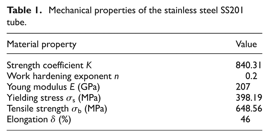
Stainless steel SS201 tubes with initial dimensions of 150 mm (length) × 32 mm (OD) × 0.75 mm (wall thickness) were adopted in the experiments. The mechanical parameters of the tube are presented in Table 1.

Table 1.

Mechanical properties of the stainless steel SS201 tube.

Material property	Value
Strength coefficient K	840.31
Work hardening exponent n	0.2
Young modulus E (GPa)	207
Yielding stress σ_s (MPa)	398.19
Tensile strength σ_b (MPa)	648.56
Elongation δ (%)	46

The loading conditions in the experiments are mainly defined by the pressure curves of hydraulic pressure P versus forming time T. As shown in Figure 2(a), five pressure curves were randomly determined. During the experiments, the tubular blank was deformed into a component with a square cross section of 32 mm × 32 mm at five different die-closing speeds. The expansion ratio of the cross section was about 27.4% assuming a uniform wall thickness for the deformed component and did not exceed the elongation value listed in Table 1, which was obtained by a uniaxial tension test.¹⁷ Figure 2(b) shows the components deformed under the five pressure curves.

Figure 2.

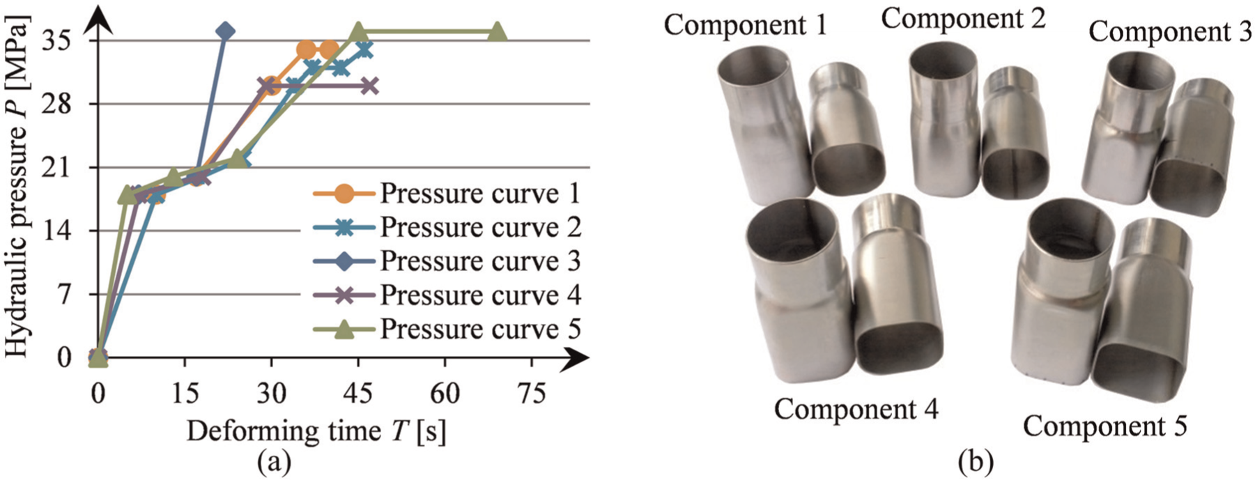
The five pressure curves adopted in the tube hydroforming with radial crushing (THFRC) experiments and the bisected components deformed under the curves: (a) the five pressure curves and (b) the bisected components.

FE model of the THFRC process

In this study, the commercial FE code DYNAFORM was used in combination with the nonlinear structural solver LS-DYNA to investigate the forming behavior and predict the optimal loading path for the THFRC process.

Material behavior was assumed to be isotropic, homogeneous, linearly elastic, nonlinearly strain-hardening, and in accord with the von Mises Yield Criterion. The FE model is shown in Figure 3. The tubular blank was meshed into grids of 1.0 mm × 1.0 mm by Belytschko–Tsay shell elements, while the tools (upper die, lower die, and sealing parts) were represented as rigid (nondeformable) materials and meshed into 15.0 mm × 5.0 mm grids by rigid shell elements. The friction coefficient µ between the blank and dies was all set to be 0.1. The total loading time and number of time steps were defined as 100 ms and 80, respectively. The initial gap between the upper and lower dies was 10 mm. The dies closed at a constant speed of 0.1 mm/ms during the THFRC simulation.

Figure 3.

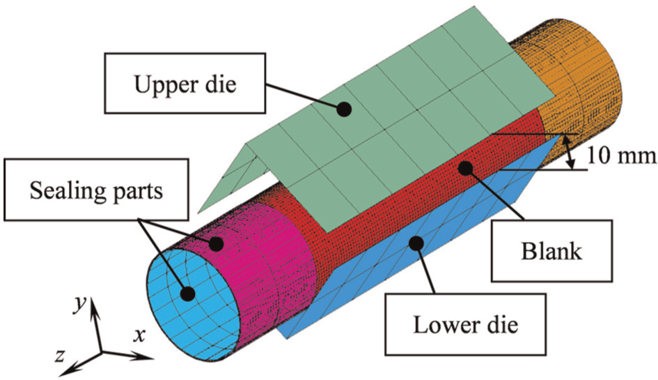
FE model of the tube hydroforming with radial crushing (THFRC) process in this study.

Validation of the FE model

To validate the FE model, FE simulations were carried out under the five pressure curves adopted in the experiments. Figure 4 shows the diagonal lengths l₁ and l₂ and wall thicknesses t_max and t_min on the middle cross section obtained from the simulation and experiment. The simulated and experimental diagonal lengths and wall thicknesses are in quite good agreement, with relative errors of <3% and <4%, respectively. Therefore, the FE model demonstrates reliability for simulating the THFRC process and can be used for predicting the loading path in the following analyses.

Figure 4.

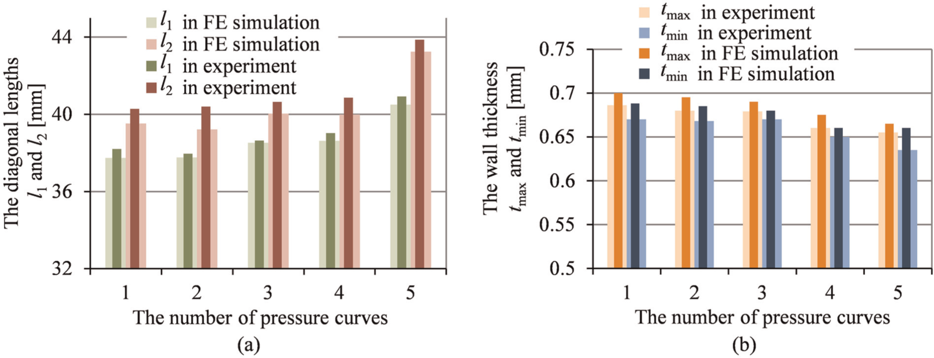
Comparison between the geometric parameters on the middle cross section of the components obtained from the FE simulations and experiments: (a) diagonal lengths l₁ and l₂ and (b) wall thicknesses t_max and t_min.

Problem description

Loading path and process window

The loading path for the THFRC process is expressed by the hydraulic pressure P versus the radial stroke S (the travel distance) of the two dies (Figure 5),¹⁹ with a maximum travel distance of 10 mm (i.e. initial gap value between the upper and lower dies). Of the five zones visible in Figure 5, the nonshaded zone is called the “process window,” which is frequently used to judge whether a loading path would lead to forming failure or not. To avoid forming failures such as jamming¹⁶ and bursting, a proper loading path for the THFRC process should fall within the process window. If P is too small or the loading path falls in the elastic zone, only elastic deformation occurs in the bulging zone of the tubular blank. By contrast, if P is too large and the loading path falls within the bursting or jamming zones, the corresponding failures occur in the bulging zone. Furthermore, if P is increased too quickly to drive the loading path to fall within the impacting zone, a hardly controllable impact load occurs in the forming process. In this study, the process window is used as a constraint for the to-be-predicted object and to limit the scope of the design variable.

Figure 5.

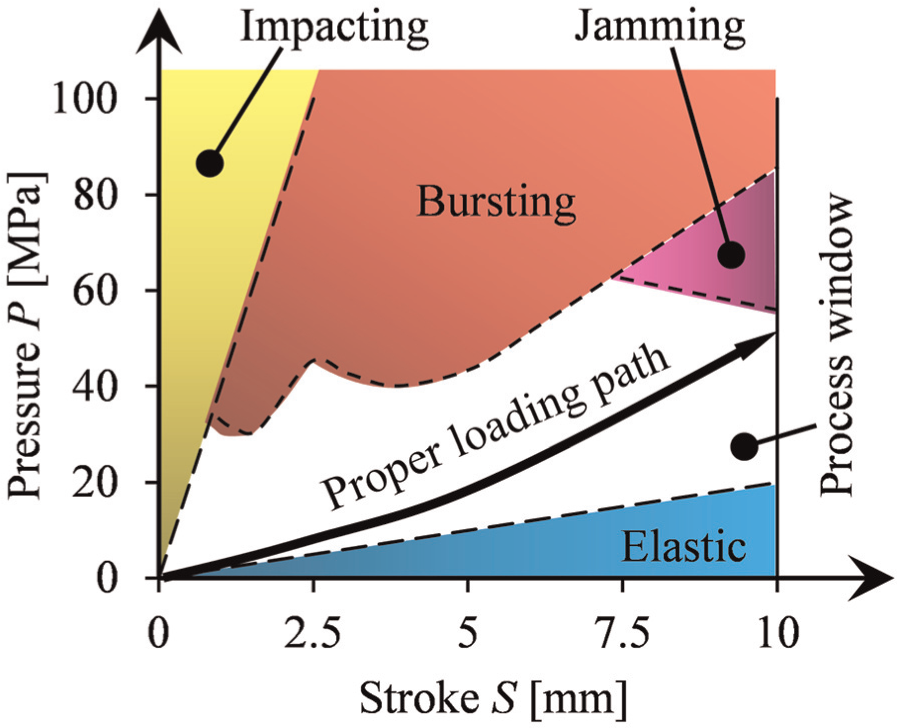
Loading path and process window of the tube hydroforming with radial crushing (THFRC) process in this study.

Formability indicators

To comprehensively evaluate the formability of the square cross-sectional component by THFRC, three formability indicators, ξ, η, and γ, are introduced to indicate the die-filling ability, cross-sectional symmetry, and wall thickness uniformity, respectively. These indicators are correspondingly defined by the following equations

ξ = \frac{(l_{1} + l_{2}) - 2 D_{0}}{2 D_{0}}

(1)

η = \frac{l_{2} - l_{1}}{D_{0}}

(2)

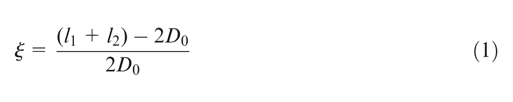
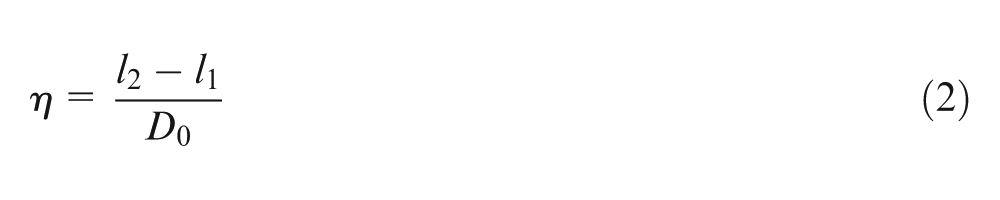
where l₁ and l₂ are the diagonal lengths on the middle cross section (see Figure 1) and D₀ is the initial OD of the tubular blank, and

γ = \frac{t_{max} - t_{min}}{t_{0}}

(3)

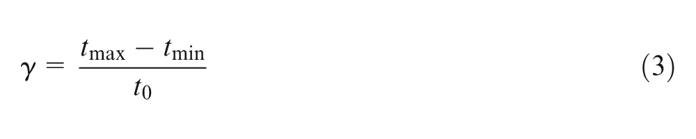
where t_max and t_min are the maximal and minimal wall thicknesses on the middle cross section of the component, respectively, and t₀ is the initial wall thickness of the tubular blank.

For THFRC, the perimeter of the deformed component without any failure is always expected to be maximal with the lowest possible hydraulic pressure. As shown in Figure 1, the larger the diagonal lengths of l₁ and l₂, the greater and better the maximum perimeter and die cavity filling, respectively. To achieve a dimensionless formability indicator, the first indicator ξ is constructed as defined in equation (1). The larger the value of ξ, the stronger the die-filling ability of the tube material.

An ideal component is characterized by a strong die-filling ability, a good cross-sectional symmetry, and excellent wall thickness uniformity, that is, a large value of ξ and small values of η and γ. Because the three formability indicators reflect the variation in the variables currently measured relative to their initial values, the formability indicator with the largest value is considered to have more influence on the formability than the other two indicators under same loading path and should be prioritized in the weight assignment.

Weighted order of the formability indicators

Although different types of loading path (e.g. linear and polygonal) would lead to somewhat different weights for the formability indicators, the weighted order should remain identical for a given component despite differences in the loading path. For convenience of calculation, a linear loading path is adopted in the present FE simulations of the THFRC process to analyze the weighted order of the formability indicators. The maximal hydraulic pressure P_max is limited to 20–50 MPa (from yielding to bursting) to obtain well-deformed components without forming failures. Variations in the formability indicators with P_max obtained from the FE simulation are shown in Figure 6.

Figure 6.

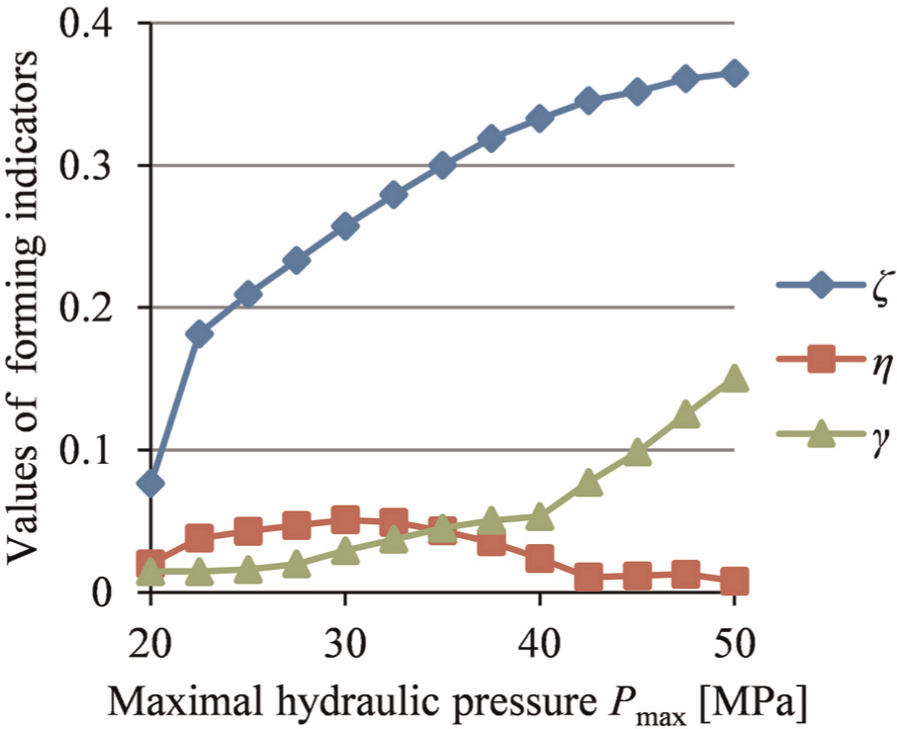
Variations in formability indicators with maximal hydraulic pressure P_max.

Figure 6 shows that the value of the die-filling indicator ξ at any P_max is larger than the values of the other two in all cases. Consequently, ξ should be given the highest priority in terms of the weighted order. When P_max < 30, η and γ can moderately be improved by decreasing the value of P_max; however, this leads to a significant deterioration of die-filling ability (or a sharp drop in ξ). Thus, the ranking for the weighted order of η and γ is neglected when P_max = 20–30 MPa. When P_max > 30 MPa, an increase in P_max can improve the cross-sectional profile but decrease the wall thickness uniformity; thus, the weighted order of γ should precede that of η.

Consequently, the formability indicators are ranked in terms of weighted order as follows: die-filling indicator ξ, wall uniformity indicator γ, and cross-sectional symmetry indicator η.

Multi-object problem definition

To evaluate the formability of the component by THFRC on the basis of the weighted order of the three formability indicators, a fractional function is introduced to define a multi-object function as follows

f = \frac{ξ}{1 + η + γ}

(4)

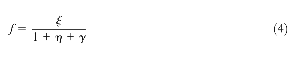
where the constant 1 is set to limit the minimal value of the denominator and thus restricts the influence of η and γ on the value of f. According to equation (4), the formability is improved if the value of f increases as the forming process proceeds. In addition, the value of f is defined to be 0 once any failure occurs in the THFRC process.

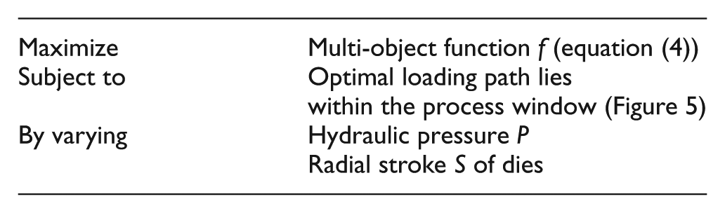
The to-be-predicted objects in this study are the optimal loading parameters under which the tubular blank can be hydroformed into a square cross-sectional component without any failure. The loading parameters are optimized by maximizing the value of f within the process window (Figure 5). Therefore, the multi-object problem is defined as follows:

Maximize	Multi-object function f (equation (4))
Subject to	Optimal loading path lies within the process window (Figure 5)
By varying	Hydraulic pressure P
	Radial stroke S of dies

Multi-strategy approach for prediction

Both GA and BM are applicable to the situation when the object function is continuous and the monotony and convexity–concavity are uncertain. The areas wherein the global optimal solution and the local optimal solution (or sub-optimal solution) lie can be roughly found by the GA process; then, the converging process of searching the local optimal solution can be accelerated by the BM method. An important characteristic of the multi-strategy approach that combines GA and BM is that it guarantees both the global optimal solution and other practicable local optimal solutions.

GA

A GA is capable of mimicking the process of natural evolution of living organisms and is frequently employed to solve global optimization problems in engineering applications. In a typical GA process, a group of individuals (or candidate solutions) are allowed to evolve to become more adaptive for an optimization problem by mutating and altering their chromosomes (or the sets of properties).

The Rosenbrock function, a continuous and nonconvex function, is used as a performance test problem for an optimization strategy to study the converging behavior of individuals in the GA process in this study. As shown in Figure 7, the extremum point a and optimum point b are known in the definition field [−2 ≤x₁≤ 2 and −2 ≤x₂≤ 2]. The performance test problem for GA is defined as follows:

Maximize:	$f (x_{1}, x_{2}) = 100 {(x_{1}^{2} - x_{2})}^{2} + {(1 - x_{1})}^{2}$
Subject to:	−2 ≤x₁≤ 2
	−2 ≤x₂≤ 2

Figure 7.

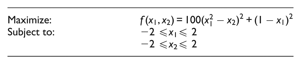
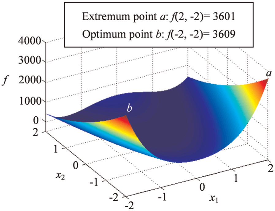
Diagram of Rosenbrock function with the extremum point a and optimum point b in the definition field.

The initialized parameters of GA in this performance test are as follows: chromosome lengths, λ = 10 for variables x₁ and x₂; population size, M = 80; maximal generation, G_max = 100; probability of crossover, p_c = 0.6; and probability of mutation, p_m = 0.001. The conditions of Figure 7 are considered known and used to justify the converging behavior of individuals in the GA process in this study.

Figure 8 shows the variations in the distribution of individuals in the definition field across generations, in which R_max represents the size of the largest among all local areas (surrounded by the dotted line). The variation in R_max reflects the convergence speed of individuals, which is characterized by a significant decrease in R_max within a few generations of the GA process. The value of R_max decreases markedly from 4 to 1.5 from the initial generation to the 5th generation (Figure 8(a) and (b)), but moderately from 1.5 to 0.9 from the 5th generation to the 100th generation (Figure 8(c) and (d)). According to Figure 7, the two local areas A and B in Figure 8(d) should contain the extremum point a and optimum point b, respectively. The Rosenbrock function evidently bears a single peak in each of the two local areas.

Figure 8.

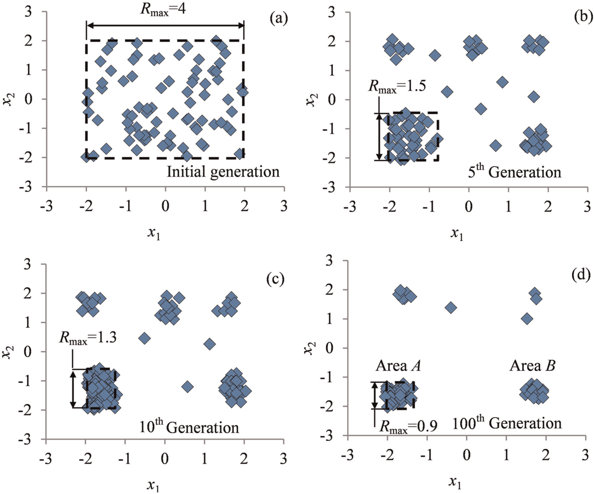
Distribution of individuals in the definition field in the genetic algorithm process for the (a) initial generation, (b) 5th generation, (c) 10th generation, and (d) 100th generation.

From the statement above, the converging behavior of individuals in the GA process may be summarized as follows: individuals have a clear tendency to converge toward local areas that are considered to bear a single peak and contain an optimal solution, and the convergence is fast for early generations but slows down for later generations.

BM

In solving an equation, the BM is often employed as an effective root searching approach because it is simple, robust, and easily programmed. In this approach, an interval is repeatedly bisected into two subintervals, one of which is then selected as that in which the root must lie for next searching process. The iteration of bisecting and selecting continues until the root for the equation is found.

The basic idea of BM is to shrink an interval under a given searching rule, for example, selecting the subinterval where the signs of the values of the function at its endpoints are opposite. By replacing the searching rule, BM can be employed effectively and easily to search for maximum or minimum values for a multi-dimensional optimization problem in a given definition field. In this study, BM is employed to search for the local optimal solution under the rule that an area where the function is nonmonotonic must be selected. Notably, the function of the optimization problem at the local area is required to be continuous and bear a single peak when a local optimal solution is expected to be obtained by using BM.

Multi-strategy approach that combines GA and BM

The multi-object function f in equation (4) is constructed with the three formability indicators obtained from the FE simulation of the THFRC process. The three formability indicators in equations (1)–(3) maintain a continuous state in a successful THFRC process unless a forming failure occurs. Hence, the f is considered to have a single peak in local areas obtained by convergence of individuals in the GA process. A search can then be made for the optimal solution in these local areas by using BM.

The basic idea of the multi-strategy approach is explained below. Because of its advantage of fast convergence early in the process, GA is applied as a constituent part of the approach to divide the definition field into several local areas. Owing to its advantages of simplicity and programmability in local searching activity, BM is then applied to search the optimal solution in those local areas. The work procedure of the multi-strategy approach for predicting the optimal loading path for the THFRC process is illustrated in Figure 9. The main steps are as follows:

As shown in Figure 9(a), a group of individuals are generated randomly in the given definition field. After a few generating operations in the GA process, the tendency of the individuals to converge divides the definition field into several local areas (e.g. local areas 1 and 2, dotted lines in Figure 9(b)). The edges of the local areas can be easily determined.

Taking local area 1 as an example, the square area containing the local area is divided into 4 × 4 meshes (Figure 9(c)). The node with maximal function value (max_node) can be found by calculating and comparing all nodes of the meshes. For local area 2, same operation is conducted in this step.

The small square area with a 2 × 2 mesh in Figure 9(c) surrounded by the bold dotted line determines which max_node is in the center. As shown in Figure 9(d), the small square area is further refined into a 4 × 4 mesh, and then, a new max_node is found by calculating and comparing all nodes of this new mesh.

The operation in step 3 is repeated until the size e of each mesh (see Figure 9(d)) becomes less than the given size determined by the accuracy requirement of the multi-object problem. Finally, the max_node of the most recent meshes is output as an optimal solution.

Figure 9.

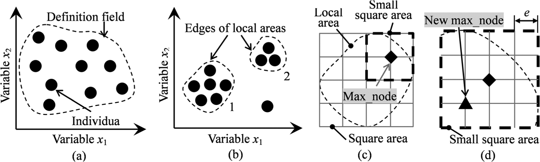
Schematic of the multi-strategy approach that combines the genetic algorithm and the bisection method for predicting optimal loading path in this study: (a) random generation of initial individuals, (b) convergence of individuals toward several local areas after a few operations, (c) division of meshes in the square area to obtain max_node, and (d) refinement of the small square area to obtain new max_node.

The initial parameters and terminating conditions of GA and BM should be determined before predicting the optimal loading path for the THFRC process. According to the basic idea of the multi-strategy approach, there is no need to obtain the accurate solution by implementing the time-consuming GA in this study. Therefore, the main parameters of GA can be roughly initialized as follows: length of chromosome, λ = 5; population size, M = 20; probability of crossover, p_c = 0.6; and probability of mutation, p_m = 0.02.

Although a small local area is beneficial in reducing the iteration times of BM in the local searching process, it requires a large number of GA generations to find the local area owing to the low convergence efficiency of individuals later in the GA process. To improve the prediction efficiency of the multi-strategy approach, a large number of generations are unnecessary. Therefore, the GA process should be terminated when the tendency of individuals to converge is evident, and the BM should subsequently be terminated when the mesh dimension e < 0.1, that is, the accuracy of the pressure P and stroke S reaches 0.1 MPa and 0.1 mm, respectively. A higher accuracy of loading parameters, which does not necessarily imply that better formability can be achieved for the component, is time-consuming and unnecessary.

Loading path prediction

Prediction for FHB stage

In the FHB stage (i.e. the tube is deformed merely by the hydraulic pressure as shown in Figure 1(a) and (b)), the degree of bulging of the tube is thought to be affected greatly by the hydraulic pressure level but less by the loading path curve. For the convenience of prediction, a linear loading path is adopted in this stage of the THFRC process. Note that the pressure level and stroke were varied during the optimization with the dies closing at a constant speed of 1 mm/s.

To diminish the undesirable effects of the friction between the tube and dies on the cross-sectional symmetry and wall thickness uniformity in the combined forming stage, the ability to directly expand the perimeter of the middle cross section to an ideal level (or 4 × 32 mm = 128 mm) without forming failures in the FHB stage would be desirable. However, this is not applicable because the perimeter would continue to increase by the hydraulic pressure at the risk of the jamming failure in the subsequent combined forming stage, and the corner radii r₁ and r₂ (Figure 1(d)) cannot be expanded to 0 mm owing to the deformation limit of the material. Hence, the perimeter is only expanded to about 125 mm (or D₁≈40 mm) in this study. The linear loading path (shown by the bold line in Figure 10), which is determined by FE simulation and meets the requirement of D₁≈ 40 mm, is adopted as an optimal loading path in the FHB stage.

Figure 10.

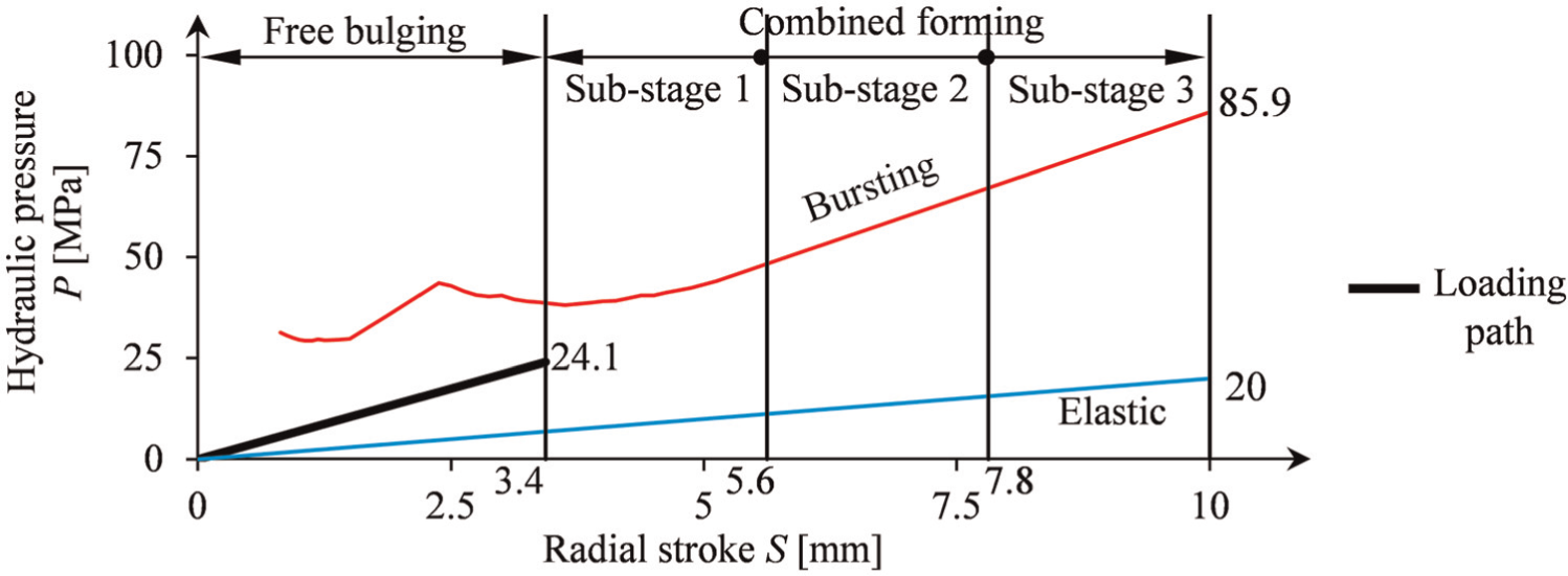
Loading paths adopted in the free hydraulic bulging stage and in sub-stages of the combined forming stage for loading path prediction.

Prediction for combined forming stage

In this study, the combined forming stage is evenly divided into three sub-stages (Figure 10). The multi-strategy approach is implemented in each sub-stage to predict the optimal loading path. Taking sub-stage 1 as an example, the prediction procedure based on FE simulation is illustrated in Figure 11. After implementing GA for five generations, the initial individuals converge to two local areas (Figure 11(a)). After implementing BM for seven iterations in each of the two local areas, the optimal loading point can be found in Area 1 (Figure 11(b)). After the prediction procedure is conducted in the same way for the other two sub-stages, the optimal loading points at the sub-stages can be found. The optimal loading path or a polygonal line in the combined forming stage is then predicted by sequentially connecting those optimal loading points in the three sub-stages. Note also that the combined forming stage can be divided into many more sub-stages for more accurate loading path.

Figure 11.

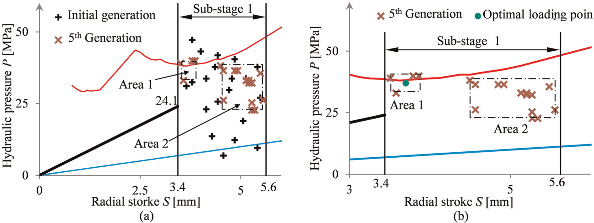
Prediction procedure in the combined forming stage (e.g. sub-stage 1): (a) initial individuals converging to two local areas after running the genetic algorithm for five generations and (b) the optimal loading point obtained after seven iterations with the bisection method in the two local areas.

Results and discussion

The optimal loading path for the THFRC process predicted by the multi-strategy method is shown in Figure 12. It is determined by sequentially connecting the linear loading path in the FHB stage and the polygonal loading path in the combined forming stage.

Figure 12.

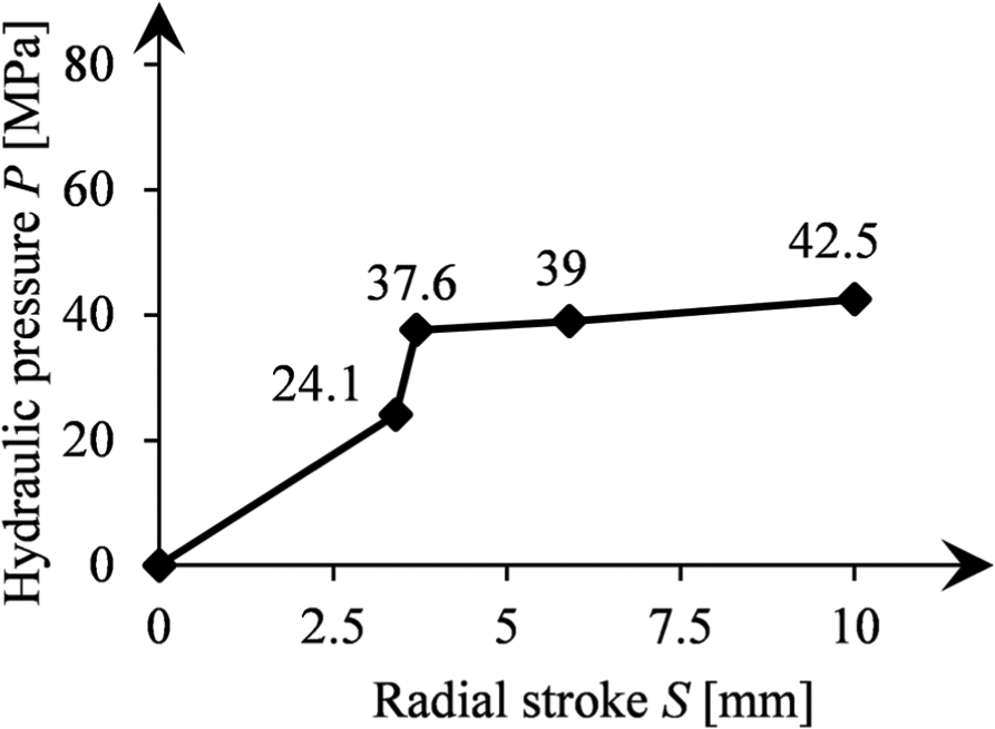
Optimized loading path for the tube hydroforming with radial crushing (THFRC) process in this study.

To verify the effectiveness of the prediction method, a comparison between the deformation parameters of the components deformed under the optimal and conventional loading paths is conducted on the basis of the FE simulation results. Four conventional loading paths, labeled as paths 1, 2, 3, and 4 in Figure 13, are selected for the verification. The maximal hydraulic pressure P_max of paths 1, 2, and 3 is identical to that of the optimal loading path. Additionally, the two components are deformed with similar values of the formability indicators ξ, η, and γ under path 4 and the optimal loading path, respectively.

Figure 13.

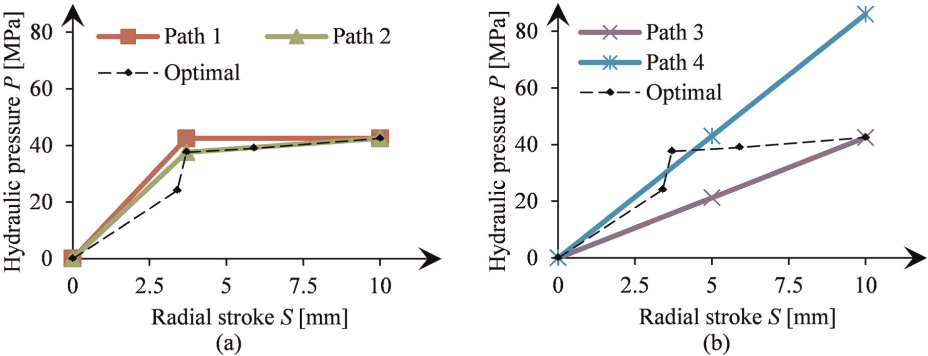
Four conventional loading paths selected to verify the effectiveness of the prediction method: (a) polygonal loading paths and (b) linear loading paths.

Figure 14 shows the middle cross-sectional profiles of the components deformed under the optimal and conventional loading paths by FE simulation, with the deformation parameters and the maximal hydraulic pressure P_max summarized in Table 2. It is comprehensible from Figure 14 and Table 2 that better formability without forming failures can be achieved with a lower loading requirement by the optimal loading path than by the conventional loading paths. Hence, the prediction method is shown to be effective.

Figure 14.

Middle cross-sectional profiles of the components deformed under the optimal and conventional loading paths by finite element simulation. The reader is referred to Table 2 for the discretion of the deformation and the formability parameters among the profiles.

Table 2.

Maximal hydraulic pressure P_max required for the deformation, as well as the deformation and formability parameters of the components deformed under the optimal and conventional loading paths.

Loading paths	P _max (MPa)	l ₁ (mm)	l ₂ (mm)	t _max (mm)	t _min (mm)	Ξ	η	Γ	f
Optimal	42.5	43.284	43.621	0.675	0.606	0.358	0.011	0.092	0.325
Path 1	42.5	43.615	43.791	0.651	0.541	0.366	0.006	0.147	0.317
Path 2	42.5	42.95	43.493	0.670	0.606	0.351	0.017	0.085	0.319
Path 3	42.5	37.353	38.786	0.704	0.692	0.19	0.044	0.016	0.179
Path 4	86	42.952	43.538	0.674	0.606	0.351	0.018	0.091	0.317

Larger value of f indicates that better formability is achieved with the deformed component.

Next, a comparison between the required total calculation times of the multi-strategy approach and GA to obtain the optimal loading path is conducted to verify the high efficiency of the former in predicting the loading path. Conventionally, the population size M and the maximal generation G_max should be larger than 20 and 100, respectively, when only GA is implemented to search for an accurate solution to an optimization problem. Thus, the optimal loading point of each sub-stage (see Figure 11), as an accurate solution of present prediction of loading path, can probably be obtained by implementing the GA process for over 2000 calculation times. By contrast, in the case of implementing the multi-strategy approach, the local areas of each sub-stage are obtained by implementing the GA process for five generations with a population size of M = 20 for each, and the optimal loading points of sub-stages 1, 2, and 3 can be found in those local areas by implementing BM for seven, six, and seven iterations, respectively. The three values for the number of iterations are determined by the local searching process of the BM. Thus, the total calculation times of the multi-strategy approach are 186, 175, and 186 in searching for the optimal loading point in sub-stages 1, 2, and 3, respectively. This demonstrates the multi-strategy approach to be highly efficient in predicting the loading path.

Conclusion

Three indicators are introduced to evaluate the formability of THFRC in terms of die-filling ability, cross-sectional symmetry, and uniformity of wall thickness. A three-step multi-strategy approach that combines a GA and the BM is proposed. In the first step, GA is applied to determine the single-peak local areas that contain optimal loading points of the loading path. In the second step, BM is used to search these points within the local areas. In the final step, the optimal loading path for the THFRC process is obtained by connecting these points in sequence. The prediction method is shown to be effective by comparing the formability of the components deformed by the optimal and conventional loading paths. The multi-strategy approach is demonstrated to be highly efficient by comparing the total number of calculations for the multi-strategy approach and for GA alone.

In this study, a linear loading path and a polygonal loading path are adopted in the FHB and combined forming stages, respectively, for convenience of FE simulations. As is known from practical experience, kinked loading paths are far less effective than curvilinear loading paths in the improvement of formability. Hence, no dramatic improvement was obtained in the objective function in this study. From a practical point of view, a proper definition of multi-object function and adoption of a curvilinear loading path are advisable. Although the optimization of curvilinear loading paths for THF is currently an enormous challenge, we intend to tackle the issue with various optimization strategies in future work.

Footnotes

Acknowledgements

The authors would like to thank Chen Fengjun and Deng Yang for their assistance with the experimental setup and graphic plots.

Declaration of conflicting interests

The authors declare that there is no conflict of interest.

Funding

This work was supported by the National Natural Science Foundation of China (grant numbers 51065006, 51271062); the Guangxi Natural Science Foundation (grant number 2013GXNSFAA019305); and the Guangxi Key Laboratory of Manufacturing System & Advanced Manufacturing Technology (grant number 11-031-12_006).

References

Morphy

. Pressure-sequence and high-pressure hydroforming. Tube Pipe J 1998; 2(1): 128–135.

Rimkus

Bauer

Mihsen

. Design of load-curves for hydroforming applications. J Mater Process Tech 2000; 108: 97–105.

Yang

Guo

. Novel approach for analysis of deformation of thin-walled tube in free hydro-bulging process. T Nonferr Metal Soc 2005; 15(3): 299–304.

Matteo

Suwat

Shr

. Virtual process development in tube hydroforming. J Mater Process Tech 2004; 146: 130–136.

Hama

Ohkubo

Kurisu

. Formability of tube hydroforming under various loading paths. J Mater Process Tech 2006; 177: 676–679.

Fann

Hsiao

. Optimization of loading conditions for tube hydroforming. J Mater Process Tech 2003; 140: 520–524.

Di Lorenzo

Ingarao

Chinesta

. A gradient-based decomposition approach to optimize pressure path and counterpunch action in Y-shaped tube hydroforming operations. Int J Adv Manuf Tech 2009; 44: 49–60.

Di Lorenzo

Ingarao

Chinesta

. Integration of gradient based and response surface methods to develop a cascade optimization strategy for Y-shaped tube hydroforming process design. Adv Eng Softw 2010; 41: 336–348.

Hossein Seyedkashi

Naeini

Liaghat

. Experimental and numerical investigation of an adaptive simulated annealing technique in optimization of warm tube hydroforming. Proc IMechE, Part B: J Engineering Manufacture 2012; 226(11): 1869–1879.

10.

Ray

Mac Donald

. Determination of the optimal load path for tube hydroforming processes using a fuzzy load control algorithm and finite element analysis. Finite Elem Anal Des 2004; 41: 173–192.

11.

Yang

Zhang

. Loading path prediction for tube hydroforming process using a fuzzy control strategy. Mater Design 2008; 29: 1110–1116.

12.

Zhang

Zhao

Zhang

. Optimization for the forming process parameters of thin-walled valve shell. Thin Wall Struct 2008; 46: 371–379.

13.

Abedrabbo

Worswick

Mayer

. Optimization methods for the tube hydroforming process applied to advanced high-strength steels with experimental verification. J Mater Process Tech 2009; 209: 110–123.

14.

Green

Johrent

. Multi-objective optimization and sensitivity analysis of tube hydroforming. Int J Adv Manuf Tech 2010; 50: 67–84.

15.

Chebbah

Naceur

Hecini

. Rapid coupling optimization method for a tube hydroforming process. Proc IMechE, Part B: J Engineering Manufacture 2010; 224(2): 245–256.

16.

Kang

Kim

Kang

. Tube size effect on hydroforming formability. J Mater Process Tech 2005; 160: 24–33.

17.

Lei

Yang

. Investigation on deformation behavior of tube in hydroforming with radial crushing. Steel Res Int 2012; 83(special edition): 655–658.

18.

Liu

Yang

. The prediction of initial yield load of a tube in hydroforming with radial crushing. Steel Res Int 2012; 83(special edition): 647–650.

19.

Tao

Yang

. Forming margin diagram for tube hydroforming with radial crushing under linear loading path. Adv Materials Res 2012; 538–541: 1106–1110.