Sage Journals: Discover world-class research

Abstract

In the present study, the Johnson-Cook damage model is proposed as a comprehensive damage criterion to predict all types of probable failures in tube hydroforming process. Also, the Johnson-Cook material model is used to predict the profile of hydroformed tubes and their dimensions. The validity of numerical results was verified using experimental results obtained in this study. Moreover, because of the importance of friction force in this process, existing between the tube and die, the friction coefficient is determined using the ring compression test, separately. The comparison of experimental and numerical results shows that Johnson-Cook damage model can predict all of the possible failures in tube hydroforming process correctly, both in terms of location and loading conditions. And this model does not predict any failure if, the tube is hydroformed perfectly. Additionally, it was cleared that the Johnson-Cook material model is a proper model to predict the profile of hydroformed tubes with remarkable accuracy. Also, it was found that the loading path and creation of a proper wrinkling have a determinative and vital role in the prosperity of the process.

Keywords

Tube hydroforming damage criterion Johnson-Cook model loading path finite element

Introduction

Tube hydroforming process is a new metal forming method of light materials leading to a considerable weight reduction.¹ So, due to increased demands for lighter parts, tube hydroforming has been widely used to manufacture parts in various fields, such as automobile, aircraft, aerospace, and shipbuilding industries.² In fact, hydroforming is the process of producing different parts of machines by applying fluid pressure.³ This fluid usually, is oil or water.⁴ Using the hydroforming process, it is possible to produce a tube component that its cross-section is varied along its axis.^5,6 Because of this unique advantage, the hydroforming process is a useful manner to manufacture integrated and seamless parts with a smaller number of production processes and more desirable mechanical properties, only in one step.⁷ Hydroforming method was originally invented to form aluminum tubes but, its usage was rapidly developed for other materials such as steel,⁸ copper,⁹ magnesium¹⁰ and titanium.¹¹ Also, the tube hydroforming process is applicable to isotropic¹² and anisotropic^13,14 materials. It is interesting to know that the tube hydroforming method can be used for very small tubes. for example, a tube with outer diameter of 0.8mm and wall thickness of 0.04 mm¹⁵ which is called micro-tube hydroforming.¹⁶

One of the most important issues in tube hydroforming process is to obtain a perfect and flawless product. For this purpose, special attention should be given to choosing the amount of forming loads including axial feeding, internal pressure and their combination. Since the forming loads apply to the tube simultaneously during hydroforming process, a suitable selection of them can guarantee the process success and an improper selection may lead to bursting or severe wrinkling. So, many researchers have studied the effects of these parameters on the tube hydroforming process experimentally and numerically, with or without a failure criterion. Guo et al.¹⁷ studied the effects of axial feeding and internal pressure on the protrusion height of the 45° Y-shape hydroformed tubes numerically. They obtained the optimized parameters for a particular geometry. Also, they determined the optimal forming loads with the specified maximum rise of the internal pressure. Guo et al.¹⁷ did this research using trial-and-error and found that the qualified Y-shapes specimen could be obtained by the optimized hydroforming process. Liu et al.¹⁸ studied the wrinkling defect in T-shape tubes using an energy criterion. Their investigation cleared that using this criterion, it is possible to predict the undesirable wrinkling may be created during the hydroforming process. Although, they did not predict the other possible damages. Shinde et al. investigated the effect of internal pressure, without axial feeding, on the success of tube hydroforming process numerically.³ They analyzed the tube hydroformed in square cross- section die using LS-Dyna explicit solver. They found that the internal pressure that can cause the tube to burst can be determined using the Formation Limit Diagram (FLD). However, they did not investigate the other types of failure.

In the present study, a new damage criterion that is Johnson-Cook damage model is introduced and used to predict the crack failure in tube hydroforming process. It should be noted that, this model includes the effects of strain rate and temperature that have been ignored in the previous studies. In addition, the Johnson-Cook material model is used to predict the profile and profile dimension of deformed tubes. All of the numerical simulations are performed using LS-Dyna software in this study. The validity of numerical results is verified by several tube hydroforming experiments conducted on steel tube samples with various axial feedings and internal pressures. Furthermore, since friction is an important factor in tube hydroforming process, the friction coefficient is determined using a ring compression test, separately.

Materials and methods

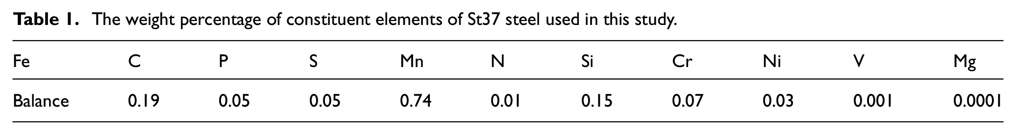
The tube material used in this study is St37 steel seamless tube with an outer diameter of 40 mm and a thickness of 1.5 mm, cut from an extruded tube. The uniaxial tensile test was conducted using an Instron machine along the axial direction of the tube and the true stress–strain curve of this material was determined. The content of the constituent elements of St37 steel, according to the quantometer test conducted in the present study, is presented in Table 1.

Table 1.

The weight percentage of constituent elements of St37 steel used in this study.

Fe	C	P	S	Mn	N	Si	Cr	Ni	V	Mg
Balance	0.19	0.05	0.05	0.74	0.01	0.15	0.07	0.03	0.001	0.0001

Tensile test

In order to determine the tensile properties and the stress-strain curve of the base material, tensile test samples were cut out from the wall of the blank tube, based on the ASTM E8 standard¹⁹ and were tested using the universal servo-hydraulic testing machine Instron. According to the recommendation of ASTM standard, the curvatures of the tensile test samples were maintained during the tensile tests. A sample of tensile test and its dimensions are shown in Figure 1. For more accuracy, three tensile tests were conducted and the obtained results were averaged.

Figure 1.

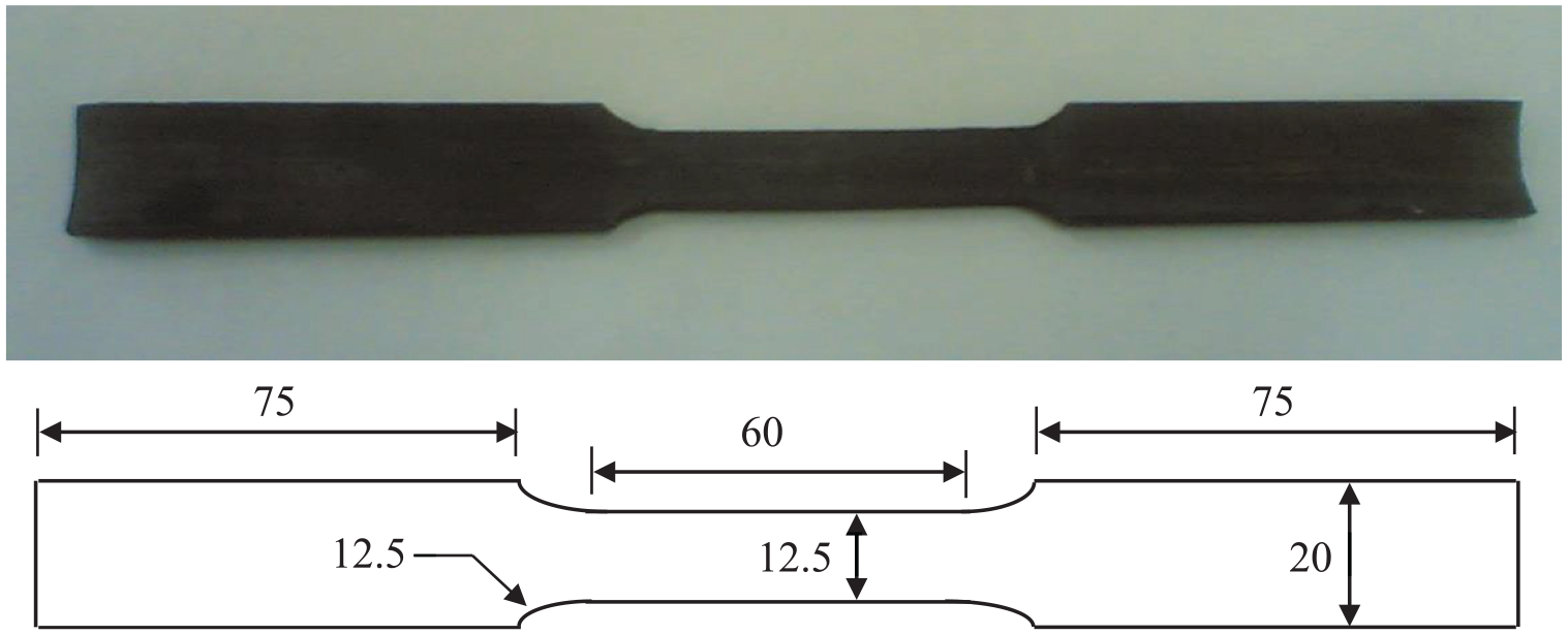
A sample of tensile test and its dimensions (in millimeter).

The anisotropy effect is taken into account by considering the Lankford coefficients measured by tensile tests relative to different directions. These coefficients are used as inputs within the FE analysis, directly. For this purpose, Lankford coefficients were measured from tensile tests performed on specimens cut in three directions corresponding to 0, 45 and 90 degree orientations from a sheet obtained by flattening the tube (Figure 2). Tensile specimens with sub-size were used for this purpose. The tube axial direction is chosen as the referential direction and the circumferential direction is a direction oriented by 90 degrees to the axial direction.

Figure 2.

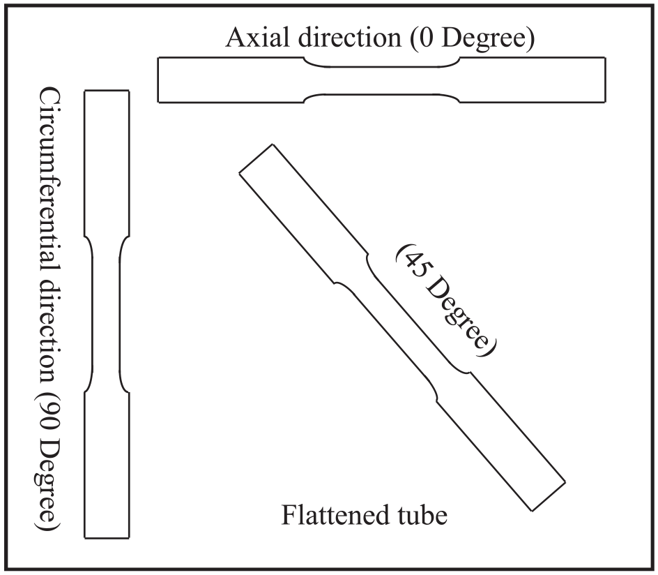
Locations of tensile test specimens cut from a sheet obtained by flattening the tube.

Friction coefficient determination

In to conduct ring compression test and to determine the friction coefficient, three ring specimens of St37 steel were submitted to mentioned tests at room temperature using a universal testing machine Instron and the results were averaged according to ASTM standard.²⁰ The disks used for ring compression tests were made of die materiel and a sample of ring compression test was made of the tubes material are shown in Figure 3. The disks and samples were lubricated by grease lubricant, right like hydroforming tests. In all tests, incremental forming methodology with mentioned lubrication at the beginning of the forming process and intermediate lubrication after every incremental step were applied. Also, the measurements of height and inner diameter change in each test steps were performed using a digital vernier caliper.

Figure 3.

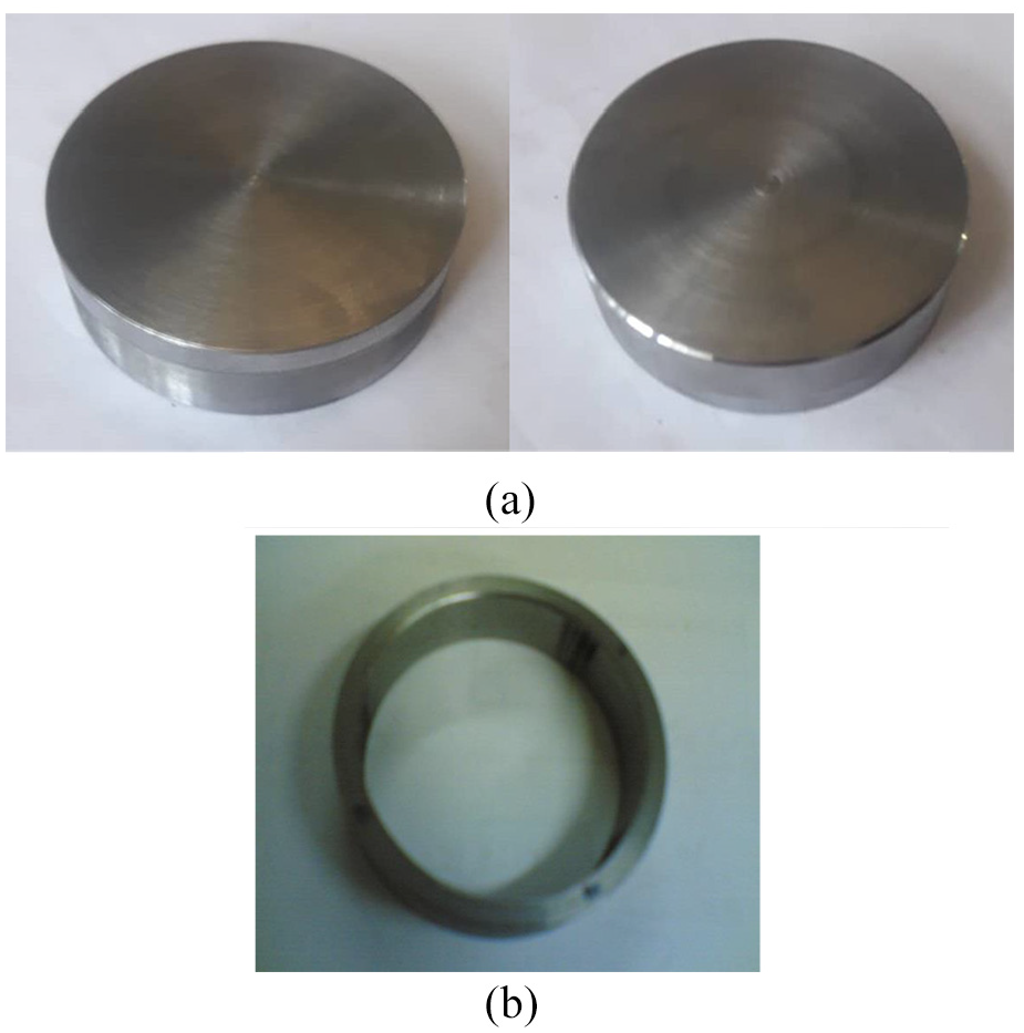
(a) The disks used for ring compression and (b) A sample of ring compression test.

Hydroforming tests

The St37 steel which is widely used in different industries and has a good formability relative to the other types of steel was used in this study. The shape of the specimens is cylindrical and the outer diameter, the thickness and the length of them are 40 mm, 1.5 mm and 200 mm, respectively. For the sealing purposes, the ends of the punches are made in conical shape. In all hydroforming tests, axial feeding was applied using a 60 tons servo-hydraulic testing apparatus Instron and the internal pressure was applied using a powerful Enerpac type pump with a capacity of 2800 bar. Figure 4(a) shows the die and punches. Also, the specimen, the die and the punches assembly is illustrated in Figure 4(b), schematically.

Figure 4.

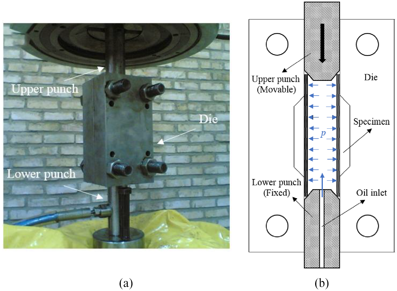
(a) Closed die and punches and (b) Schematic of specimen, die and the punches assembly used in the hydroforming tests.

Hydroforming tests were conducted on the blank tube using the mentioned apparatus. Some of the tests were conducted with the excessive axial feeding to study the occurrence of the wrinkling and some of the tests were conducted with the excessive internal pressure to study the bursting phenomenon. In addition to these tests, several of specimens were hydroformed by different combinations of axial feeding and internal pressure. The amounts of internal pressure are presented versus the axial feeding in diagrams named loading path, in this study.

Simulations

Hydroforming process was simulated using the Ls-Dyna software. For this purpose, the punches, the die and the blank tube were considered and modeled. Because of symmetry, in all simulations, only 1/4 of the blank tube was modelled. The 1/4 of the blank tube was modelled using 1125 thin shell element. The die and the punches were simulated as rigid bodies. The contact surfaces between the die and the specimen are defined by “Contact-automatic surface to surface” elements. Also, the coefficient of friction between the die and blank tube was considered as 0.168. This value was obtained by the ring compression test. Right like the hydroforming experiments, the lower punch hasn’t any motion and was kept fixed during the hydroforming process and just the upper punch can move. The motion of the upper punch is along the axis of symmetry. In these simulations, there is no need to simulate the forming oil as a separate part and it is enough to consider its effect. The effect of forming oil can be taken into account as “segment pressure.” Using this option of LS-Dyna software, the internal pressure can be applied to the inner surface of the blank tube according to a diagram in which shows the amounts of internal pressure versus the time.

The Johnson-Cook material model is used in the present simulations. This material model can be expressed as follows:

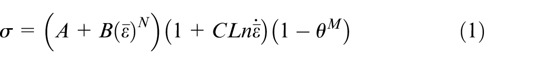
σ = (A + B {(\bar{ε})}^{N}) (1 + CLn \overset{\cdot}{\bar{ε}}) (1 - θ^{M})

(1)

Where A, B, C, N and M are material constants and can be determined experimentally. $\bar{ε}$ is the equivalent plastic strain and $\overset{\cdot}{\bar{ε}}$ is the plastic strain rate. Also, $θ$ is the homologous temperature defined as $θ = \frac{T - T_{room}}{T_{melt} - T_{room}}$ where $T_{melt}$ is the melt temperature and $T_{room}$ is the room temperature. In this study, $T_{melt}$ and $T_{room}$ are considered as 1350°C and 27°C respectively.²¹

The main aim of this study is the prediction of different failure modes which may happen during the hydroforming process so, a comprehensive damage criterion is needed. It seems that Johnson-Cook failure model is suitable for this purpose. This failure model is given as:

ε^{f} = {\begin{matrix} (D_{1} + D_{2} \exp (D_{3} σ^{*})) (1 + D_{4} Ln ({\overset{\cdot}{ε}}^{*})) (1 + D_{5} θ) & σ^{*} < 1.5 \\ ε_{min}^{f} & σ^{*} \geq 1.5 \end{matrix}

(2)

Where, $D_{1}$ to $D_{5}$ and $ε_{min}^{f}$ are the material constants in which should be determined, experimentally. Also, $σ^{*}$ is the stress triaxiality factor defined as:

σ^{*} = \frac{P}{\bar{σ}}

(3)

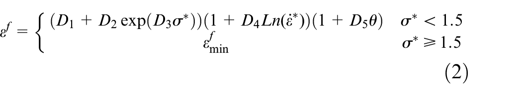
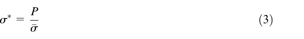
where P is the hydrostatic pressure, $P = (σ_{1} + σ_{2} + σ_{3}) / 3$ and $\bar{σ}$ is the Von Mises stress. The discontinuity of $ε^{f}$ at $σ^{*}$ = 1.5 is due to the assumed constant failure strain treatment of the spall failure process. It should be noted that, piecewise continuity of $ε^{f}$ at $σ^{*}$ = 1.5 is established if:

ε_{min}^{f} = (D_{1} + D_{2} \exp (D_{3} 1.5)) (1 + D_{4} Ln ({\overset{\cdot}{ε}}^{*})) (1 + D_{5} θ)

(4)

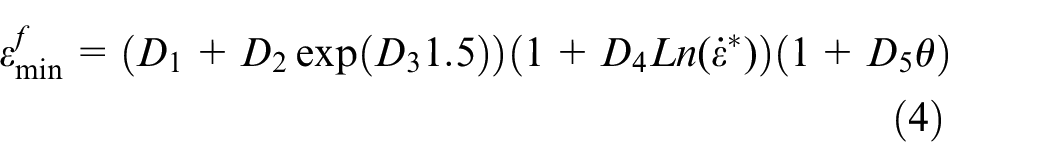
According to this damage model, failure occurs when the damage parameter, which defined as $D = \frac{\bar{ε}}{ε_{f}}$ , reaches to 1. In LS-Dyna software, D in step n+1 $(D^{n + 1})$ is calculated as:

D^{n + 1} = D^{n} + Δ D

(5)

Where:

\begin{matrix} Δ D = {\begin{matrix} Δ \bar{ε} (D_{1} + D_{2} \exp (D_{3} σ^{*^{n + 1}})) (1 + D_{4} Ln (\frac{Δ \bar{ε}}{Δ t {\overset{\cdot}{\bar{ε}}}_{0}})) (1 + D_{5} θ^{n + 1}) & σ^{* tr} < 1.5 \\ \frac{Δ \bar{ε}}{ε_{min}^{f}} & σ^{* tr} \geq 1.5 \end{matrix} \end{matrix}

(6)

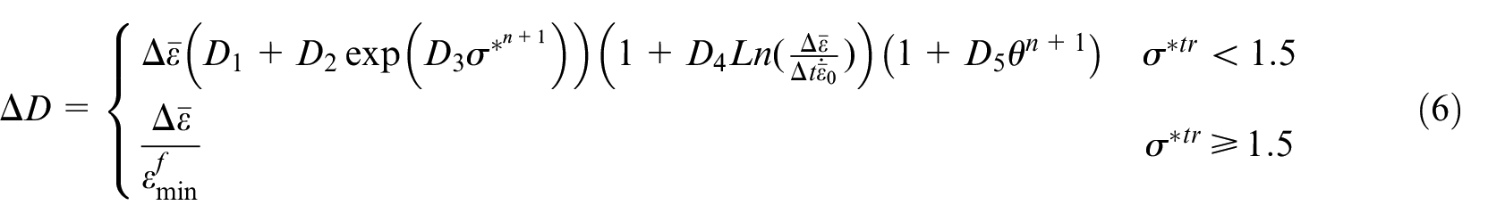
In equation (6) “tr” indicates to trial values. So, in the present study, the Johnson-Cook material model was used to predict the profile shapes and dimensions of hydroformed tubes and Johnson-Cook damage model was used to predict the possible failure during the hydroforming process.

Results and discussions

Tensile test

Figure 5 shows the diagram of real stress versus real strain for base metal and its fitted Johnson-Cook curve. Based on the fitted curve and using Table Curve 2D software, the constants of the Johnson-Cook model can be determined. Accordingly, these constants are: A = 239.6MPa, B = 573.9 MPa and n = 0.812.

Figure 5.

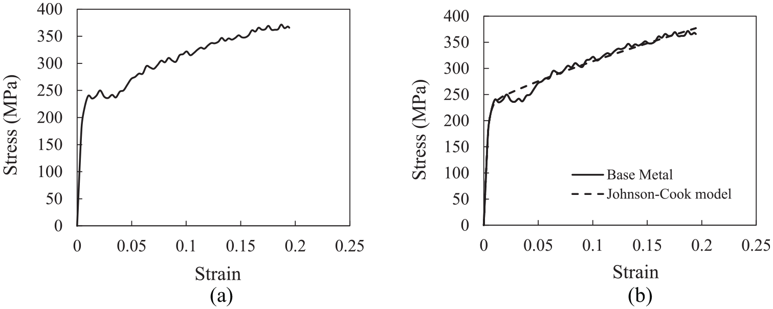
(a) True stress-strain curves for base metal and (b) True stress-strain curves for base metal and its fitted Johnson-Cook curve.

It should be noted that, since the hydroforming tests are conducted slowly and tubes temperature changes are negligible during the hydroforming process, usually, the second and the third parentheses in Johnson-Cook material model are considered equal to one. This matter may lead to some errors in obtained results so, in the present study, for more accuracy and precision and paying attention to the high speed of experiments, all parts of the Johnson-Cook model are taken into account and therefore, the C and the m are considered as 0.002 and 1.035, respectively. In order to determine the C parameter, the ﬂow stresses at 0.05 of the equivalent plastic strain are plotted against the natural logarithm of the dimensionless strain rate, in Figure 6. The constant C can be obtained by ﬁtting linearly the ﬂow stresses at 0.05 equivalent plastic strain of dynamic tests at room temperature (see Figure 6). The 0.05 equivalent plastic strain value was chosen to avoid the oscillations that appear at low strains in the dynamic true nominal stress–strain curves. Avoiding such oscillations means that the ﬂow stress was measured in a constant strain rate condition. The model can be expressed only as a function of the dimensionless strain rate as follows:

σ = (A + B {(0.05)}^{N}) (1 + CLn \overset{\cdot}{\bar{ε}})

(7)

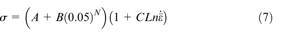
where the weakening and the thermal softening effects are considered negligible due to the low equivalent plastic strain and the same temperature (ambient temperature) for all these tests. Figure 6 shows the ﬁtting of the model and experimental data. Accordingly, the C parameter can be determined as 0.002.

Figure 6.

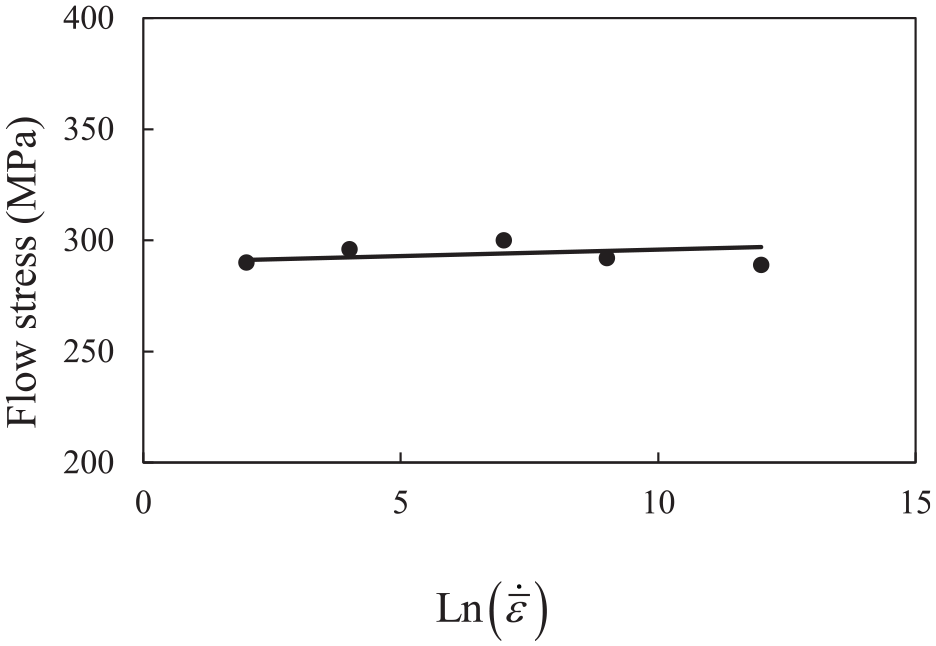
Experimental values of the flow stress at ε = 0.05 against the natural logarithm of the dimensionless strain rate.

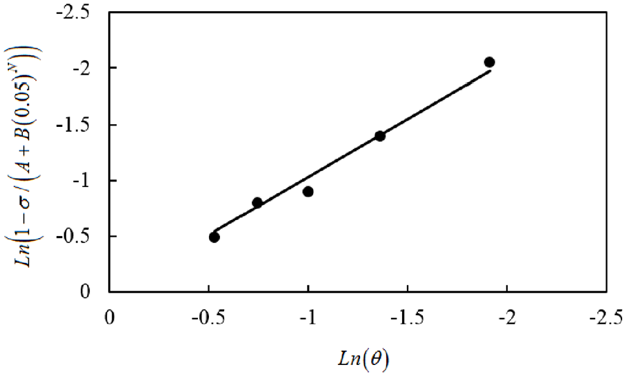
In order to determine the M parameter, in a similar manner, the quantities of $Ln (1 - σ / (A + B {(0.05)}^{N}))$ are plotted against the natural logarithm of the dimensionless temperature, in Figure 7. The constant M can be obtained by ﬁtting linearly the ﬂow stresses at 0.05 equivalent plastic strain of various natural logarithm of the dimensionless temperature. According to this, the M parameter can be determined as 1.035.

Figure 7.

Experimental values of $Ln (1 - σ / (A + B {(0.05)}^{N}))$ against the natural logarithm of the dimensionless temperature.

This study is a part of a teamwork and in a separate but related part of this study, the failure constants of Johnson-Cook model equation (2) were determined as: $D_{1} - 1.3$ , $D_{2} = 2.37$ , $D_{3} - 0.5$ , $D_{4} = 0.002$ and $D_{5} = 0.61$ .

Constants $D_{1}$ , $D_{2}$ and $D_{3}$ were determined by performing quasi-static tensile tests of constant strain-rate on notched specimens with different notch radius and without notch specimens at constant room temperature. After obtaining experimental data of the stress triaxiality factor for all tensile specimens of both notched and without notch specimens, the failure strain $(ε^{f})$ versus stress triaxiality factor $(σ^{*})$ data was curve fitted and used to determine parameters of $D_{1}$ , $D_{2}$ and $D_{3}$ (Figure 8). In this case, equation (2) becomes:

ε^{f} = (D_{1} + D_{2} \exp (D_{3} σ^{*}))

(8)

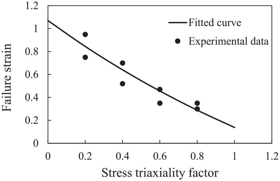
Based on the described method, the constants $D_{1}$ to $D_{3}$ were evaluated as: $D_{1} - 1.3$ , $D_{2} = 2.37$ and $D_{3} - 0.5$ .

Figure 8.

Variation of failure strain with stress triaxiality factor.

Constant $D_{4}$ was determined by conducting dynamic tensile tests at room temperature under different strain rates and a certain stress triaxiality factor. After specifying data of the failure strain at these different strain rates, the experimental points were curve fitted (Figure 9) and the parameters of $D_{4}$ was determined. In this case, equation (2) becomes:

ε^{f} = (D_{1} + D_{2} \exp (D_{3} σ^{*})) (1 + D_{4} Ln ({\overset{\cdot}{ε}}^{*}))

(9)

So, the constant $D_{4}$ was determined as: $D_{4} = 0.002$ .

Figure 9.

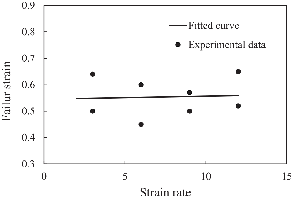
Variation of failure strain with strain rate.

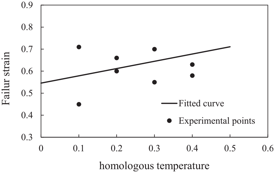
Finally, constant $D_{5}$ was evaluated by conducting tensile tests under reference strain rate at deferent temperatures. After obtaining the data of failure strain at different homologous temperatures tests, the experimental points were curve fitted (Figure 10) and the parameter $D_{5}$ was determined as: $D_{5} = 0.61$ .

Figure 10.

Variation of failure strain with homologous temperature.

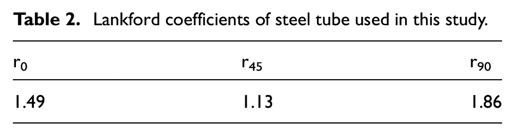
The Lankford anisotropy coefficient R-value is defined as the ratio of the strain in the width direction to that in the thickness direction. Therefore, three Lankford coefficients (r₀, r₄₅ and r₉₀) are calculated and listed in Table 2. These coefficients can be used directly, by LS-Dyna software in tube hydroforming simulations.

Table 2.

Lankford coefficients of steel tube used in this study.

r₀	r₄₅	r₉₀
1.49	1.13	1.86

Friction coefficient determination

In simulation process of compression tests, different parts of this process including dies and workpiece and conditions of tests were defined step by step. In order to determine the calibration curves, simulations for different values of the Coulomb friction coefficient were performed. Based on obtained simulations results, calibration curves are determined and drawn in Figure 11. In addition, experimental results obtained by ring compression tests are presented in this figure.

Figure 11.

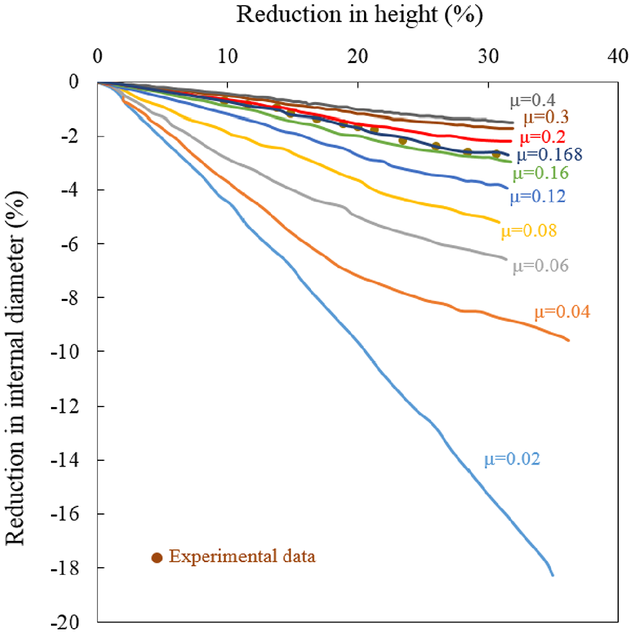
Comparative graphs between calibration curves and experimental data of friction coefficient.

It should be noted that, some experimental data in which were out of the expected range, were passed up. Paying attention to Figure 11 and using the interpolation method, it can be concluded that the Coulomb friction coefficient is 0.168. The friction coefficient is an important parameter in the simulation of the hydroforming process and should be determined carefully for this purpose. Figure 12 shows a deformed ring after the ring compression test.

Figure 12.

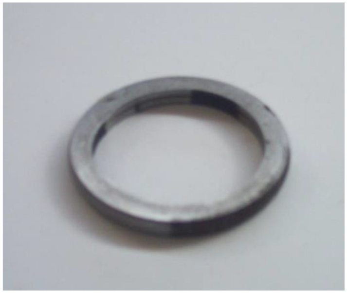
A deformed ring after the ring compression test.

Hydroforming tests and numerical simulations

In order to perform a comprehensive investigation, hydroforming experiments were conducted in three categories. In the first category, excessive axial feeding was exerted to the tubes without enough internal pressure and it is clear that the tubes were failed because of severe wrinkling in this case. In the second category, only internal pressure was exerted. In this case, the tubes were burst and it wasn’t a suitable loading path to obtain a perfect hydroformed specimen. Finally, in the third category, a combination of axial feeding and internal pressure simultaneously were applied to the tubes. The results of this case were strongly depended on the loading path. Based on the applied loading path, some of the tubes were formed well and some of them were formed improperly. In this section, these three categories loading and their obtained results are investigated, respectively.

Since the main goal of this research is the validation of Johnson-Cook’s material and damage models in hydroforming process, all of the categories of hydroforming tests were simulated using this material model and the occurred failures were predicted by its damage model. So, in this study, the numerical and the experimental results were compared with each other from two points of view. Firstly, can the Johnson-Cook material model predict the appearance shapes of the hydroformed tubes, correctly? Secondly, can the Johnson-Cook damage model predict all of the kinds of possible failures occurring in the hydroformed tubes under various loading paths, accurately?

Axial feeding

In these hydroforming experiments series, initial blank tubes were subjected to forming loads according to a loading path that included a considerable axial feeding and a low internal pressure. This internal pressure is too low to form the tubes and axial force of the punches is the dominant factor. In this category of experiments, the blank tubes cannot fill the cavity of the die. The reason of this matter is a severe wrinkling occurred owing to excessive axial feeding. This severe wrinkling leads to tubes failure. Figure 13(b) and (d) show two examples of hydroformed tubes of this category. As these two images indicate, both of the tubes were failed in the top of the wrinkling. The loading paths of these samples are presented in Figure 13(a) and (c).

Figure 13.

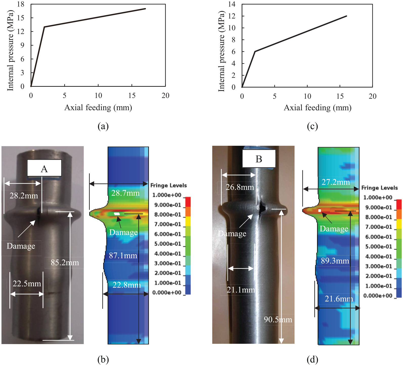
(a) Load curve, (b) experimental sample and its numerical model (damage parameter distribution) failed because of excessive axial feeding (17.3 mm), (c) load curve, and (d) experimental samples and its numerical model (damage parameter distribution) failed because of excessive axial feeding (16.1 mm).

In Johnson-Cook damage model, when the damage parameter value reaches to 1 in a certain element and failure occurs, that element will be eliminated and deleted from the numerical model. So, it is possible to determine the damage location and moment. In fact, the deleted element indicates the beginning location of damage and the loading conditions that leads to failure. Figure 13(b) and (d) presents a comparison between the experimental sample and its numerical model for two hydroformed tubes. As these figures show, both experimental samples have failed because of the excessive axial feeding and the failure location is in the top of the wrinkling of the tubes. Also, the deleted elements in these figures indicate that numerical models predict the damage occurrence and the interesting point is that the deleted elements are located on the top of the wrinkling of the tubes, just like what happens in the experiments. So, it can be concluded that in this case, the Johnson-Cook damage model can predict the damage and its location, correctly.

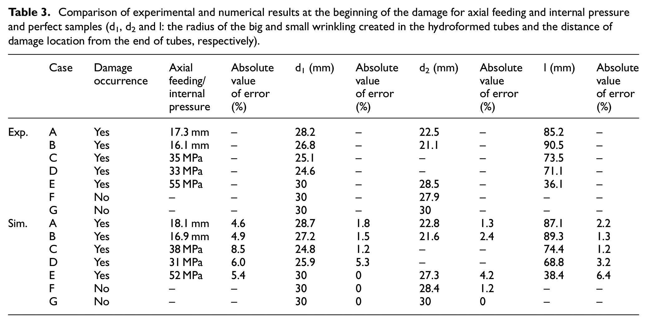
In order to validate the Johnson-Cook material model accuracy, the profiles of the numerical and experimental hydroformed tubes were compared with each other. The radii of the top of the wrinkling were measured for this purpose and were compared with each other. The results of these measurements and comparisons are presented in Figure 13 and Table 3. This figure and this table indicate that there is a considerable agreement between the numerical and the experimental profiles of the deformed specimens and also between their dimensions. Table 3 shows that the maximum absolute value of error in prediction of profile dimension is 4.9%.

Table 3.

Comparison of experimental and numerical results at the beginning of the damage for axial feeding and internal pressure and perfect samples (d₁, d₂ and l: the radius of the big and small wrinkling created in the hydroformed tubes and the distance of damage location from the end of tubes, respectively).

	Case	Damage occurrence	Axial feeding/internal pressure	Absolute value of error (%)	d₁ (mm)	Absolute value of error (%)	d₂ (mm)	Absolute value of error (%)	l (mm)	Absolute value of error (%)
Exp.	A	Yes	17.3 mm	–	28.2	–	22.5	–	85.2	–
	B	Yes	16.1 mm	–	26.8	–	21.1	–	90.5	–
	C	Yes	35 MPa	–	25.1	–	–	–	73.5	–
	D	Yes	33 MPa	–	24.6	–	–	–	71.1	–
	E	Yes	55 MPa	–	30	–	28.5	–	36.1	–
	F	No	–	–	30	–	27.9	–	–	–
	G	No	–	–	30	–	30	–	–	–
Sim.	A	Yes	18.1 mm	4.6	28.7	1.8	22.8	1.3	87.1	2.2
	B	Yes	16.9 mm	4.9	27.2	1.5	21.6	2.4	89.3	1.3
	C	Yes	38 MPa	8.5	24.8	1.2	–	–	74.4	1.2
	D	Yes	31 MPa	6.0	25.9	5.3	–	–	68.8	3.2
	E	Yes	52 MPa	5.4	30	0	27.3	4.2	38.4	6.4
	F	No	–	–	30	0	28.4	1.2	–	–
	G	No	–	–	30	0	30	0	–	–

Internal pressure

In the second hydroforming tests category, the forming loads were applied to the initial blank tubes according to a loading path that includes high internal pressure and low axial feeding. This low axial feeding was applied to the tubes for sealing, only. It is clear that the sealing process is an important matter in tube hydroforming tests. In this experiment series, the initial tubes cannot fill the die, right like the previous series. In this category of hydroforming experiments, the high internal pressure without enough axial feeding leads to a severe thinning in the wall of the tubes. It is clear that in tubes hydroforming, the axial feeding prevents severe thinning occurring in the tubes during the hydroforming process. Therefore, the lack of enough axial feeding leads to a considerable thinning in the tube wall. Owing to this severe thinning the tubes will burst and the hydroforming process will fail. Figure 14(b) and (d) show two samples of hydroformed tubes of this test series. As this figure shows, both of the tubes were failed because of bursting. Also, the related loading paths of these two samples are shown in Figure 14(a) and (c) respectively. As Figure 14 indicates, in both cases, the Johnson-Cook damage model has predicted the damage occurred due to high internal pressure both in terms of occurrence and location. Also, the comparison of the predicted profile of tubes and what obtained from the experiments shows that the Johnson-Cook material model can predict the profile of tubes in this category too. The radii of the top of the wrinkling were measured and were compared with together for numerical and experimental specimens. The results of these measurements are presented in Figure 14 and Table 3. This table indicates that there is a remarkable agreement between the numerical and the experimental profiles of the deformed specimens. Also, Table 3 shows that the maximum absolute value of error in prediction of the profile dimension is 5.3% and in the prediction of critical internal pressure is 8.5% in this category.

Figure 14.

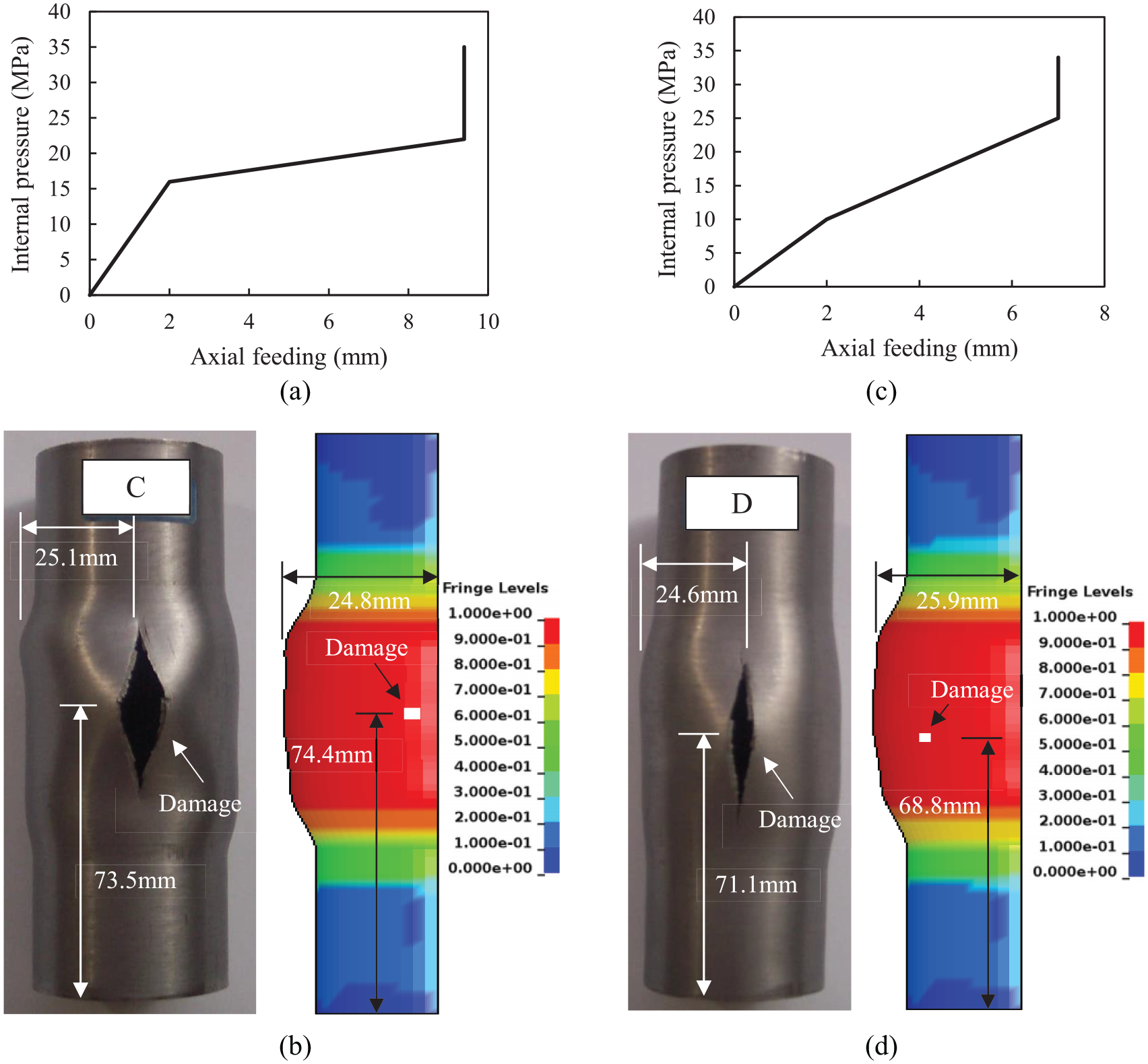
(a) Load curve, (b) experimental sample and its numerical model (damage parameter distribution) failed because of high internal pressure (35 MPa), (c) load curve, and (d) experimental samples and its numerical model (damage parameter distribution) failed because of high internal pressure (33 MPa).

Axial feeding and internal pressure

As mentioned before, in the third tests category, the initial blank tubes were subjected to forming loads according to the loading paths that includes high internal pressure and a considerable axial feeding. Only, in these conditions, it is possible to achieve a perfect hydroformed specimen. In this category, using a suitable loading path, the initial blank tubes can fill completely the cavity of the die. However, all of the hydroforming tests in this category didn’t lead to obtain an optimal and desirable results. Based on experience, it was found that to obtain a perfect result, the loads should be exerted in such a way that a moderate wrinkling be created in the blank tube firstly, and in the next step, internal pressure increases and tube expands. In the expanding step, the created wrinkling disappears and tube fills the cavity of the die, perfectly. This expanding step is called “calibration step”.

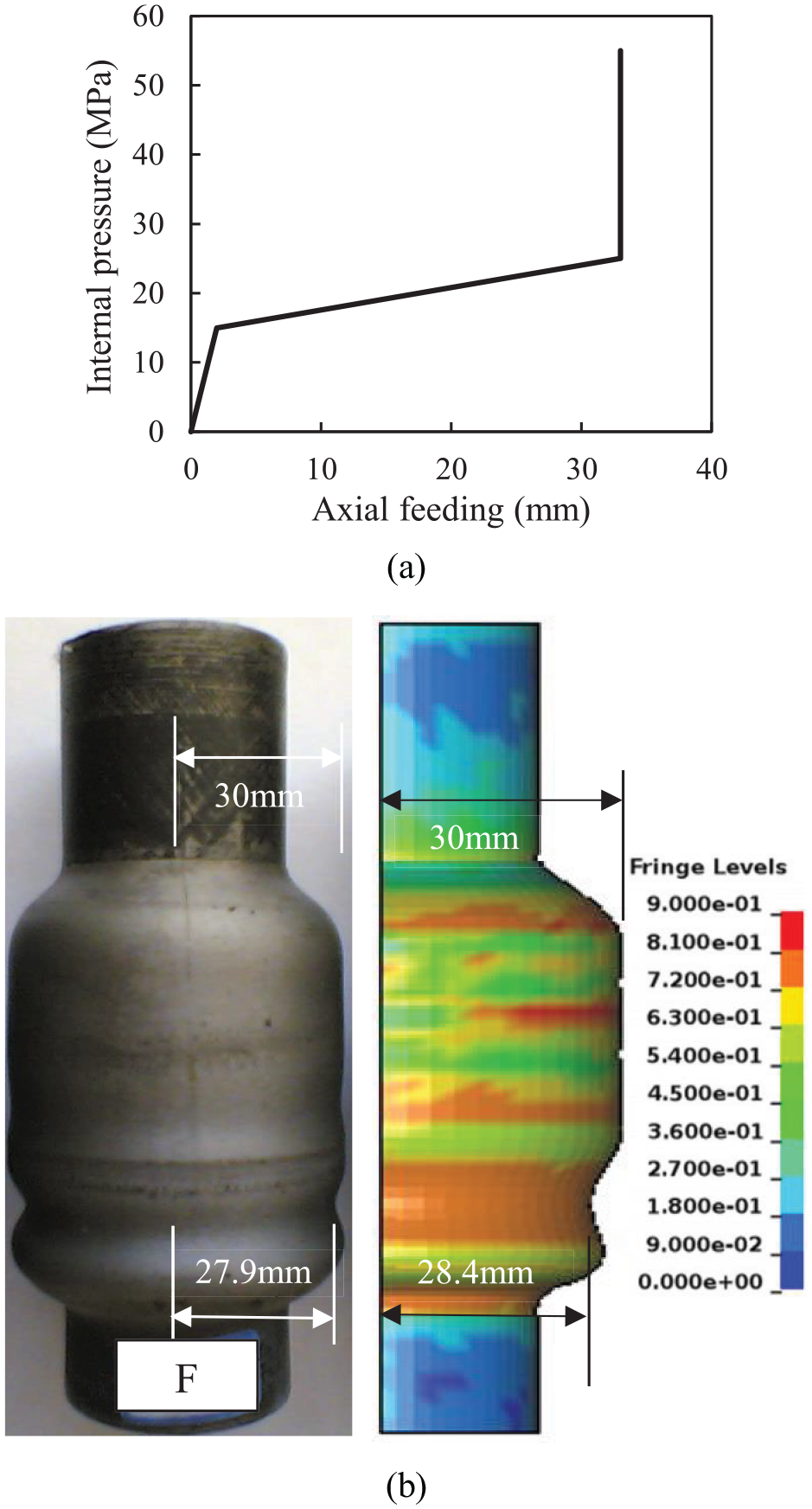
If the created wrinkling is inadequate, the tube bursts in the calibration step. An instance of this case is shown in Figure 15(b) and its loading path is presented in Figure 15(a). This tube is burst owing to severe thinning occurred in its wall. On the other hand, if the created wrinkling in the tube is sharp and severe, it will not be vanished in the calibration step and will remain in the hydroformed tube. This case can be seen in Figure 16(b). As this figure shows, the irremovable wrinkling remains in the tube as a defect. Figure 16(a) shows the loading path of this case.

Figure 15.

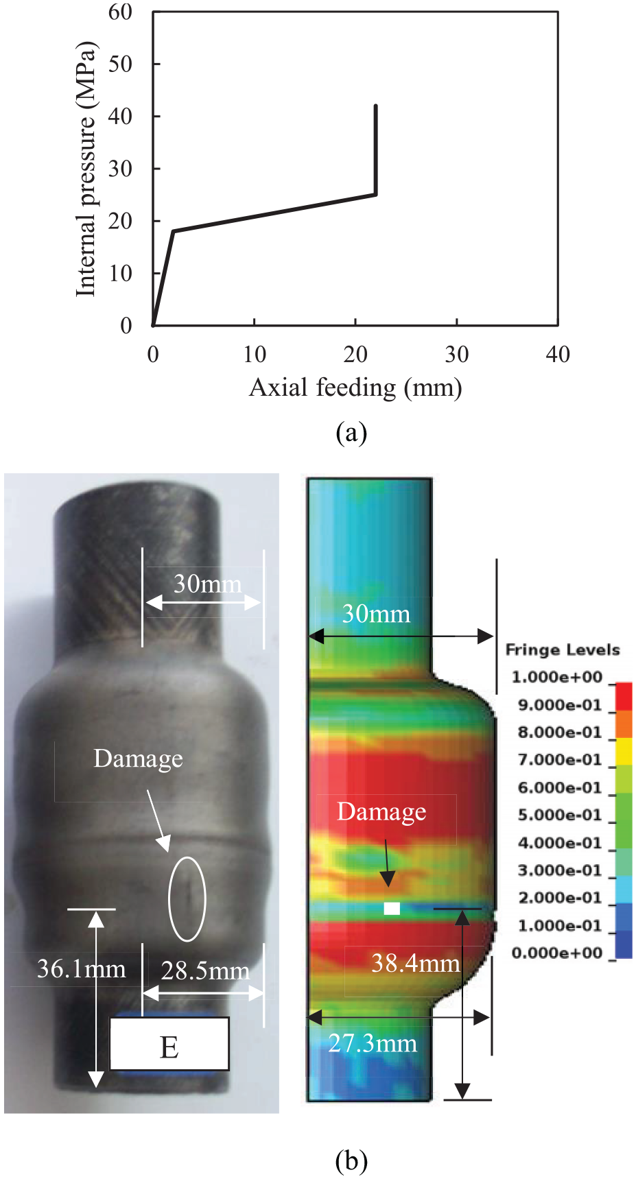
(a) Load curve and (b) experimental sample and its numerical model (damage parameter distribution) failed because of high internal pressure (55 MPa).

Figure 16.

(a) Load curve and (b) experimental sample with irremovable wrinkling and its numerical model.

In spite of two previous samples, using a suitable loading path and creation of a moderate wrinkling, it is possible to obtain a perfect and successful hydroformed sample. One of the successful samples in which perfectly has filled the hydroforming die is shown in Figure 17. As mentioned, in this case, a moderate wrinkling was created in the tube at the beginning of the process and then, using internal pressure, the tube expanded and wrinkling vanished and tube filled completely the die.

Figure 17.

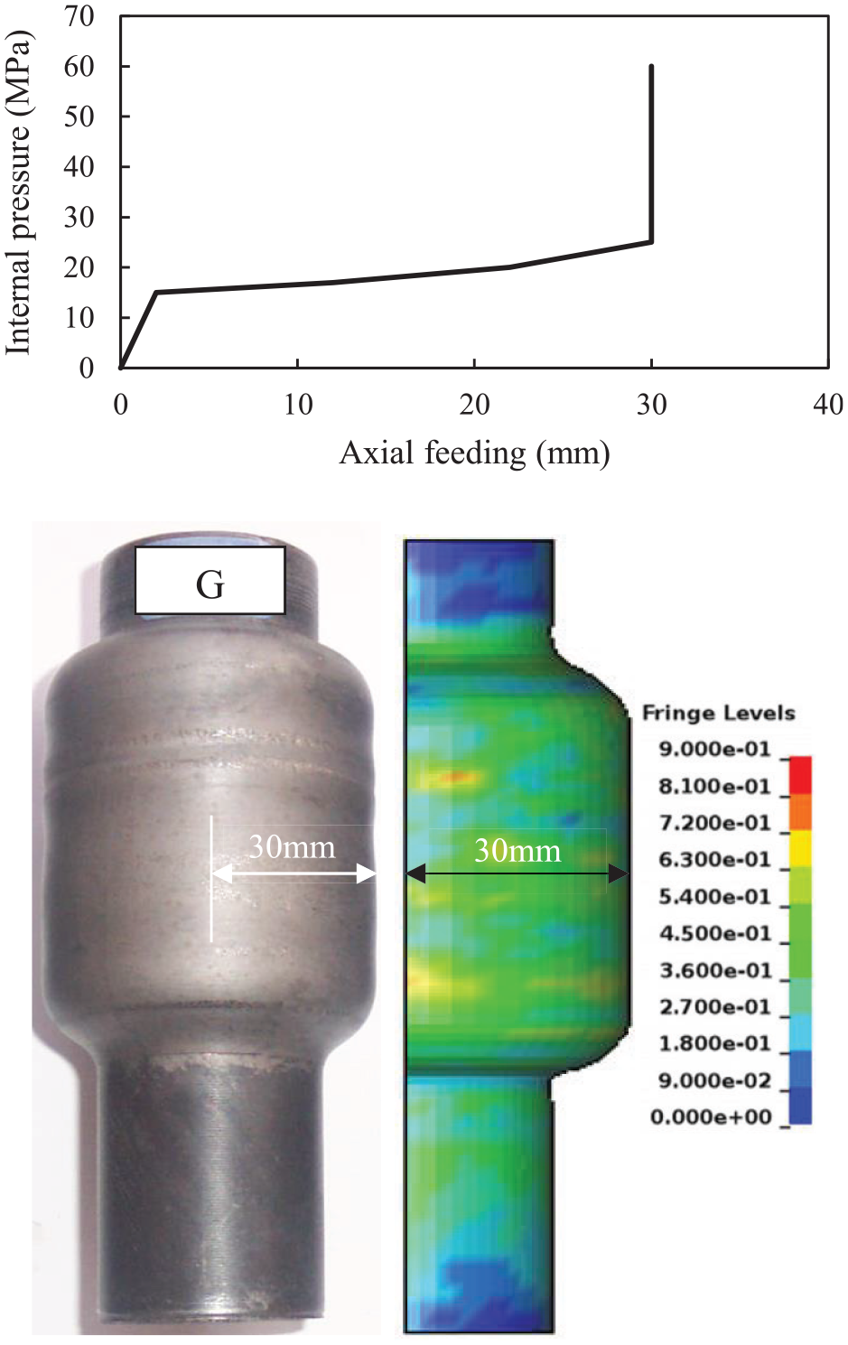
Experimental sample and its numerical model in which has filled the die perfectly.

The numerical models of the resent three cases are shown in Figures 15 –17, respectively. In these cases, like two previous categories, the Johnson-Cook material and damage models can predict the profile of deformed tubes, and occurred damage. The comparison of experimental and numerical results of this category are presented in Table 3. This table indicates that in these cases the maximum absolute value of error in prediction of profile dimension is 4.2% and the absolute value of error in prediction of critical internal pressure is 5.4% for this case.

In Table 3, the location of occurred damage in experimental specimens and the predicted location of damage in simulated specimens are presented and compared. Due to axisymmetry, this comparison can be done using only one number. This number is the distance of damage location from the end of the tube. These distances are shown in specimens in which damaged occurred in Figures 13 –15. Also, these distances are presented in Table 3 and compared. Table 3 shows that the predicted locations of damage are close to the locations of damage occurred in experiments. The most absolute value of error in these predictions is 6.4% that is insignificant. This mater indicates that the Johnson-Cook damage model can predict the location of damages, acceptably.

Table 3 shows that the Johnson-Cook damage model is successful in prediction of occurrence or non-occurrence of failure. Also, this damage model can predict when and where damage will happen. Therefore, the Johnson-Cook damage model is a suitable model that can be used to predict the various failures in tube hydroforming process. In addition, this table indicates that there is a considerable agreement between the numerical and the experimental results from the point of view tube profile dimensions. This matter shows that the Johnson-Cook material model can estimate the profile of deformed tubes and their dimensions correctly.

In order to investigate the ability of the Johnson-Cook material model more effectively, predicted thickness profiles were compared with thickness profiles obtained from experiments for all hydroforming cases (with and without damage). For this purpose, after the hydroforming experiments ending, the hydroformed tubes were cut axially and their thickness along the tube length were determined. Also, the corresponding values of these thicknesses were determined numerically and both profiles thickness were compared for each hydroforming cases. These comparisons are presented in Figure 18. This figure indicates that these profiles are very close together and the predicted thickness profile and experimental thickness profile correspond to each other in all hydroforming cases, acceptably. This matter shows that the Johnson-Cook material model can predict the thickness of the hydroformed tubes, successfully. So, the Johnson-Cook material model is an appropriate model for tube hydroforming process simulation.

Figure 18.

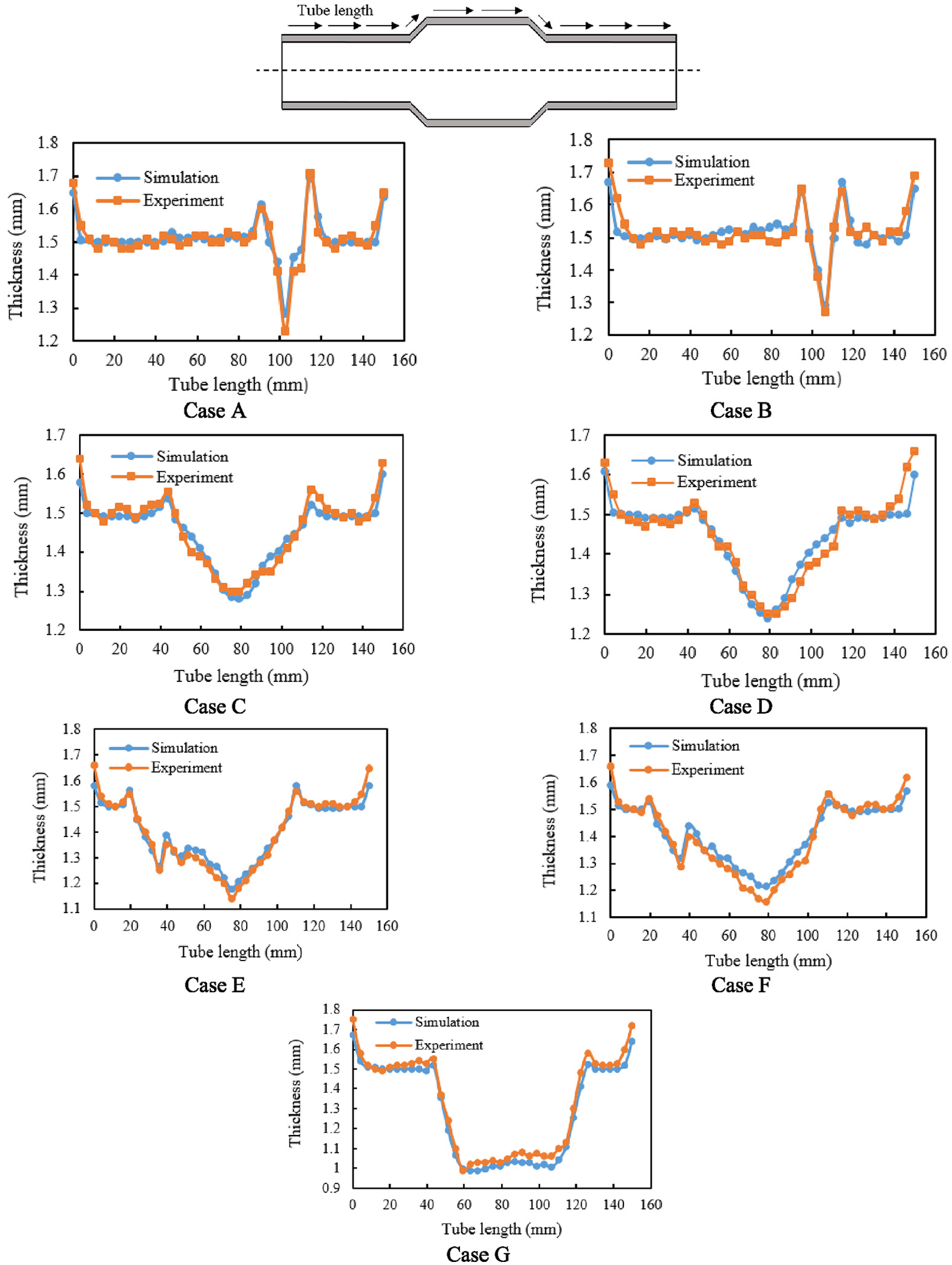
Thickness distribution for numerical and experimental results.

For a better comparison of the loading paths, all of the used loading paths are presented in Figure 19. The legends in this figure indicate the written letter on each hydroformed specimens in the previous figures. As Figure 19 clearly shows, in loading paths A and B the axial feeding is too much relative to the internal pressure and this intense axial feeding leads to fracture, as it was seen. Also, in loading paths C and D excessive internal pressure without enough axial feeding is the reason of bursting. In loading path E, although the forming factors are exerted simultaneously, because of the lack of a useful wrinkling, the tube was burst. In addition, Figure 19 shows that in loading path F the amount of axial feeding is massive, although, the needed internal pressure is exerted too. As it was seen, in this case an irremovable wrinkling is created in the hydroformed tube in which is owing to this massive axial feeding. Finally, in loading path G that forming factors that include internal pressure and axial feeding are applied simultaneously and correctly, using a useful wrinkling, a perfect and complete hydroformed specimen can be obtained. This specimen has been shown in Figure 17.

Figure 19.

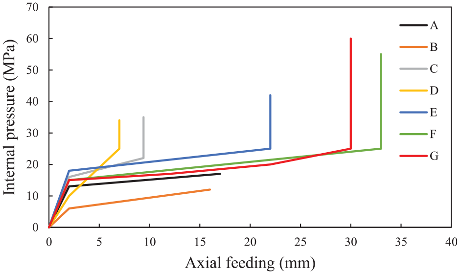
Different loading paths applied in this study.

Conclusion

The following conclusions can be derived from this study:

1- Johnson-Cook damage model can predict all of the possible failures in tube hydroforming process correctly, both in terms of location and loading conditions and this model does not predict any failure if, the tube is hydroformed perfectly. This study showed that the maximum error in prediction of damage location is 6.4% and therefore, it is expected that the numerical method developed here can be used as an effective tool for evaluating the formability of many tubes to be hydroformed.

2- It was proved that the Johnson-Cook material model is an appropriate model to predict the profile shape and dimensions of deformed tubes with remarkable accuracy. In addition, this material model can predict the thickness distribution acceptably and it can be concluded that the proposed approach is an appropriate approach for industrial application.

3- Loading path diagram presents the amounts of internal pressure versus axial feeding during the hydroforming process and is a very important and vital factor in this process. So, using the Johnson-Cook damage model, it is possible to predict numerically that which loading path can lead to obtain a perfect final product and which loading path cannot. Therefore, many cost and time can be saved.

4- Creation of a moderate wrinkling can help to obtain a perfect and successful final production in tube hydroforming process. Although, it is important how to create it. Therefore, in practical tube hydroforming process, in order to avoid excessive thinning, it is strongly recommended to create wrinkling in the tube wall firstly, and to remove the wrinkling by raising the internal pressure in the next step.

5- Undoubtedly, the accuracy of obtained simulation results in this work is beholden of the determination of the exact friction coefficient. So, it can be concluded that in order to obtain an accurate simulation, the friction coefficient should be determined experimentally and exactly for the used material.

6- Generally, loading paths that can lead to obtain successful sample production can be divided into three main parts. The first one is sealing part that includes about 2 mm axial feeding and a little internal pressure. The second one is wrinkling part in which consists of a considerable axial feeding and low increasing in internal pressure and the third one is final forming part that internal pressure increases significantly without any axial feeding.

Footnotes

Declaration of conflicting interests

The author(s) declared no potential conflicts of interest with respect to the research, authorship, and/or publication of this article.

Funding

The author(s) received no financial support for the research, authorship, and/or publication of this article.

ORCID iD

Reza Pourhamid

References

Ashrafi

Khalili

Investigation on the effects of process parameters in pulsating hydroforming using Taguchi method. Proc IMechE, Part B: J Engineering Manufacture 2015; 230: 1203–1212.

Liu

Yang

, et al. Investigation of tube hydroforming along with stamping of thin-walled tubes in square cross-section dies. Proc IMechE, Part B: J Engineering Manufacture 2016; 230: 111–119.

Jang

Lee

Park

GJ.

Optimization of the loading path for the tube-hydroforming process. Proc IMechE, Part D: J Automobile Engineering 2016; 230(12): 1605–1623.

Fazlollahi

Morrovati

Dariani

BM.

Theoretical, numerical and experimental investigation of hydro-mechanical deep drawing of steel/polymer/steel sandwich sheets. Proc IMechE, Part B: J Engineering Manufacture 2018; 233: 1529–1546.

Shahri

SEE

Boroughani

SYA

Khalili

, et al. Ultrasonic tube hydroforming, a new method to improve formability. Proc Technol 2015; 19: 90–97.

Prabhu

Muhandri

Sing

, et al. Decision support system enabled by depth imaging sensor data for intelligent automation of moving assemblies. Proc IMechE, Part B: J Engineering Manufacture 2016; 232: 51–66.

Marini

Cunninghum

Corney

JR.

Near net shape manufacturing of metal: a review of approaches and their evolutions. Proc IMechE, Part B: J Engineering Manufacture 2017; 232: 650–669.

Grzancic

Lobbe

Ben Khalifa

, et al. Analytical prediction of wall thickness reduction and forming forces during the radial indentation process in Incremental Profile Forming. J Mater Proc Technol 2019; 267: 68–79.

Peng

, et al. An investigation on the formability of sheet metals in the micro/meso scale hydroforming process. Int J Mech Sci 2019; 150: 265–276.

10.

Wang

Yang

Bai

, et al. Evaluation of limit deformation behavior in hydro-bulging of the double-layer sheet metal using diffuse and localized instability theories. Int J Mech Sci 2019; 150: 145–153.

11.

Djavanroodi

Ebrahimi

Janbakhsh

A contribution to multi-channel sheet hydroforming. Proc Manuf 2019; 29: 248–255.

12.

Venkateshwar Reddy

Veerabhadra Reddy

Srinivasa Rao

. A numerical study on tube hydroforming process to optimize the process parameters by Taguchi method. Mater Today Proc 2018; 5: 25376–25381.

13.

Shao

Bai

, et al. Experimental investigation of forming limit curves and deformation features in warm forming of an aluminum alloy. Proc IMechE, Part B: J Engineering Manufacture 2016; 232: 465–474.

14.

Cui

Wang

Yuan

SJ.

Further assessment of the plastic instability of thin-walled tubes in double-sided hydro-bulging process with verification experiments. Proc IMechE, Part B: J Engineering Manufacture 2018; 233: 776–786.

15.

Ngaile

Lowrie

Punch design for floating based micro-tube hydroforming die assembly. J Mater Proc Technol 2018; 253: 168–177.

16.

Lowrie

Ngaile

Scalability of conventional tube hydroforming processes from macro to micro/meso. Proc IMechE, Part B: J Engineering Manufacture 2017; 232: 2164–2177.

17.

Guo

Tao

Yuan

, et al. Hydroforming simulation and preparation of low activation martensitic steel Y-shapes. Nucl Eng Des 2011; 241: 2802–2806.

18.

Liu

Peng

Yuan

, et al. Analysis on critical conditions of sidewall wrinkling for hydroforming of thin-walled Tee-joint. Int J Mach Tool Manuf 2015; 97: 42–49.

19.

ASTM E8-16a. Standard test methods for tension testing of metallic materials. West Conshohocken, PA: ASTM International, 2018.

20.

ASTM E9-09. Standard test methods of compression testing of metallic materials at room temperature. West Conshohocken, PA: ASTM International, 2018.

21.

Incropera

DeWitt

Bergman

, et al. Foundations of heat transfer. Chichester: Wiley Textbooks, 2013.

A comprehensive damage criterion in tube hydroforming

Abstract

Keywords

Introduction

Materials and methods

Tensile test

Friction coefficient determination

Hydroforming tests

Simulations

Results and discussions

Tensile test

Friction coefficient determination

Hydroforming tests and numerical simulations

Axial feeding

Internal pressure

Axial feeding and internal pressure

Conclusion

Footnotes

Declaration of conflicting interests

Funding

ORCID iD

References