Sage Journals: Discover world-class research

Abstract

This article deals with an economic production quantity inventory model for non-instantaneous deteriorating items under inflationary conditions, permissible delay in payments, customer returns, and price- and time-dependent demand. The customer returns are assumed as a function of demand and price. The effects of time value of money are studied using the Discounted Cash Flow approach. The main objective is to determine the optimal selling price, the optimal length of the production period, and the optimal length of inventory cycle simultaneously such that the present value of total profit is maximized. An efficient algorithm is presented to find the optimal solution of the developed model. Finally, a numerical example is extracted to solve the presented inventory model using our proposed algorithm, and the effects of the customer returns, inflation, and delay in payments are also discussed.

Keywords

Inventory permissible delay in payments economic production quantity non-instantaneous deteriorating items customer returns inflation pricing

Introduction

In the past few years, the deteriorating inventory systems have been studied considerably. Deterioration refers to the spoilage, damage, dryness, vaporization, and loss of utility of the products, such as vegetables, foodstuffs, meat, fruits, alcohol, radioactive substances, gasoline, and so on. The first authors who investigated the inventory models for deteriorating items were Ghare and Schrader.¹ Following Ghare and Schrader,¹ several efforts have been made on developing the inventory systems for deteriorating items, for example, in studies by Covert and Philip,² Hariga,³ Heng et al.,⁴ Jaggi et al.,⁵ Moon et al.,⁶ Sarker et al.,⁷ and Wee.⁸ Goyal and Giri⁹ provided a detailed survey of deteriorating inventory literatures.

Optimal pricing is an important revenue enhancing business practice that is often combined with inventory control policy. Therefore, several researchers have studied the pricing and inventory control problems of deteriorating items. Shi et al.¹⁰ developed the optimal pricing and ordering strategies with price-dependent stochastic demand and supplier quantity discounts. Dye¹¹ considered the optimal pricing and ordering policies for deteriorating items with partial backlogging and price-dependent demand. Heng et al.⁴ and Abad¹² discussed the pricing and lot-sizing inventory model for a perishable good allowing shortage and partial backlogging. Dye et al.¹³ investigated the optimal pricing and inventory control policies for deteriorating items with shortages and price-dependent demand. Chang et al.¹⁴ developed the inventory model for deteriorating items with partial backlogging and log-concave demand. Samadi et al.¹⁵ proposed the pricing, marketing, and service planning inventory model with shortages in fuzzy environment. In this model, the demand is considered as a power function of price, marketing expenditure, and service expenditure. Tsao and Sheen¹⁶ considered the problem of dynamic pricing, promotion, and replenishment for deteriorating items under the permissible delay in payments.

In the real world, the majority of products, such as fruits, foodstuffs, green vegetables, and fashionable goods, would have a span of maintaining original state or quality, that is, there is no deterioration occurring during that period. Wu et al.¹⁷ introduced the phenomenon as “non-instantaneous deterioration.” For these types of items, the assumption that the deterioration starts from the instant of arrival in stock may lead to an unsuitable replenishment policy due to overstating relevant inventory cost. Thus, it is necessary to consider the inventory problems for non-instantaneous deteriorating items.

Moreover, in the traditional inventory model, it was implicitly assumed that the payment must be made to the supplier for items immediately after receiving the items. However, in real life, the supplier could encourage the retailer to buy more by allowing a certain fixed period for settling the account, and there is no charge on the amount owed during this period.

Recently, some researchers have studied the problem of joint pricing and inventory control for non-instantaneously deteriorating items under permissible delay in payments. Ouyang et al.¹⁸ presented the inventory model for non-instantaneous deteriorating items considering permissible delay in payments. Chang et al.¹⁹ investigated the inventory model for non-instantaneous deteriorating items with stock-dependent demand. Yang et al.²⁰ developed the optimal pricing and ordering strategies for non-instantaneous deteriorating items with partial backlogging and price-dependent demand. Geetha and Uthayakumar²¹ considered the economic order quantity (EOQ) inventory model for non-instantaneous deteriorating items with permissible delay in payments and partial backlogging. Musa and Sani²² discussed the inventory model for non-instantaneous deteriorating items with permissible delay in payments. Maihami and Nakhai Kamalabadi²³ presented the joint pricing and inventory control model for non-instantaneous deteriorating items with price- and time-dependent demand and partial backlogging. In addition, the mentioned model was extended by Maihami and Nakhai Kamalabadi²⁴ under permissible delay in payments.

In all of the models mentioned above, the inflation and the time value of money were ignored. It has happened mostly because most of decision makers believe that inflation does not have considerable influence on the inventory policy and thus do not consider the effect of inflation on the inventory system. But, today, inflation has become a perpetual feature of the economy. As a result, it is important to consider the effect of inflation and time value of money on the inventory policy and financial performance. The first author who considered the effect of inflation and time value of money on an EOQ model was Buzacott.²⁵ Following Buzacott,²⁵ several efforts have been made by researchers to reformulate the optimal inventory management policies taking into account inflation and time value of money, for example, in studies by Misra,²⁶ Park,²⁷ Datta and Pal,²⁸ Goal et al.,²⁹ Hall,³⁰ Sarker and Pan,³¹ Hariga and Ben-Daya,³² Horowitz,³³ Moon and Lee,³⁴ Mirzazadeh et al.,³⁵ Sarkar and Moon,³⁶ Sarkar et al.,³⁷ Taheri-Tolgari et al.,³⁸ and Gholami-Qadikolaei et al.³⁹ Wee and Law⁴⁰ presented a joint pricing and inventory control model for deteriorating items under inflation and price-dependent demand. Hsieh and Dye⁴¹ developed the pricing and inventory control problem for deterioration considering price- and time-dependent demand and time value of money. Hou and Lin⁴² presented the optimal pricing and ordering strategies for deteriorating items under inflation and permissible delay in payments. Ghoreishi et al.⁴³ proposed the joint pricing and inventory control model for deteriorating items taking into account inflation and customer returns. In this model, shortage is allowed and partially backlogged, and the demand is a function of both time and price. Ghoreishi et al.⁴⁴ addressed the problem of joint pricing and inventory control model for non-instantaneous deteriorating items under time value of money and customer returns. In this model, shortages are not allowed and the demand is deterministic and depends on time and price simultaneously.

Returns of product from customers to retailers are a significant problem for many direct marketers. Hess and Mayhew⁴⁵ used regression models to show that the number of returns has a strong positive linear relationship with the quantity sold. Anderson et al.⁴⁶ conducted empirical investigations that show that customer returns increase with both the quantity sold and the price set for the product. Chen and Bell⁴⁷ investigated the pricing and order decisions when the quantity of returned product is a function of both the quantity sold and the price. Zhu⁴⁸ considered the joint pricing and inventory control problem in a random and price-sensitive demand environment with return and expediting.

In this article, we develop an appropriate pricing and inventory control model for an economic production quantity (EPQ) model with non-instantaneous deteriorating items, permissible delay in payments, inflation, and customer returns. In the traditional inventory model, it was assumed that the payment must be made to the supplier for items immediately after receiving the items. However, in real life, the supplier could encourage the retailer to buy more by allowing a certain fixed period for settling the account, and there is no charge on the amount owed during this period. Therefore, in order to incorporate the realistic conditions, the delay in payment should be considered. Moreover, in practice, the majority of deteriorating items would have a span, in which there is no deterioration. For this type of items, the assumption that the deterioration starts from the instant of arrival in stock may lead to make inappropriate replenishment policies due to overvaluing the relevant inventory cost. As a result, in the field of inventory management, it is necessary to incorporate the inventory problems for non-instantaneous deteriorating items. On the other hand, the combination of price decisions and inventory control can yield considerable revenue increase due to optimizing the system rather than its individual elements. Also, the empirical findings of Anderson et al.⁴⁶ show that customer returns increase with both the quantity sold and the price set for the product. Moreover, in order to address the realistic circumstances, the effect of time value of money should be considered. Thus, a finite planning horizon inventory model for non-instantaneous deteriorating items with price- and time-dependent demand rate is developed. In addition, the effects of permissible delay in payments, customer returns, and time value of money on replenishment policy are also considered. We assume that the customer returns increase with both the quantity sold and the product price. An optimization algorithm is presented to derive the optimal length of the production period, selling price, and the number of production cycles during the time horizon, and then the optimal production quantity is obtained when the total present value of the total profit is maximized. Thus, the replenishment and price policies are appropriately developed. A numerical example is provided to illustrate the proposed model. The results of this example are used to analyze the impact of customer returns, inflation, and delay in payments on the optimal solution.

Following this, in section “Analysis method and assumptions,” the analysis method and assumptions used are presented. In section “The model formulation,” we establish the mathematical model. Next, in section “The optimal solution procedure,” an algorithm is presented to find the optimal selling price and inventory control variables. In section “A numerical example,” we give a numerical example and, finally, we provide a summary and some suggestions for future work in section “Conclusion and outlook.”

Analysis method and assumptions

Analysis method

In this article, we develop a mathematical model that provides a decision support system fostered by Operational Research that could be implemented in management sciences, business administration, and economics. Therefore, we investigate an appropriate pricing and inventory control model for an EPQ model with non-instantaneous deteriorating items, permissible delay in payments, inflation, and customer returns. The notations used in this article are defined in Appendix 1.

Assumptions

A single non-instantaneous deteriorating item is assumed.

The initial and final inventory levels both are zero.

The production rate, which is finite, is higher than the demand rate.

Delivery lead time is zero.

The planning horizon is finite.

The demand rate, $D (p, t) = (a - bp) e^{λ t}$ (where $a, b > 0$ ), is a linearly decreasing function of the price and decreases (increases) exponentially with time if λ < 0 (λ> 0), respectively.¹⁶

Shortages are not allowed.

The length of the production period is larger than or equal to the length of time in which the product exhibits no deterioration, that is, $t_{p} \geq t_{d}$ .

Following the empirical findings of Anderson et al.,⁴⁶ we assume that customer returns increase with both the quantity sold and the price. We use the general form $RC (p, t) = α D (p, t) + β p (β \geq 0, 0 \leq α < 1)$ that is presented by Chen and Bell.⁴⁷ Customers are assumed to return $RC (p, t)$ products during the period for full credit, and these units are available for resale in the following period. We assume that the salvage value of the product at the end of the last period is S per unit.

The model formulation

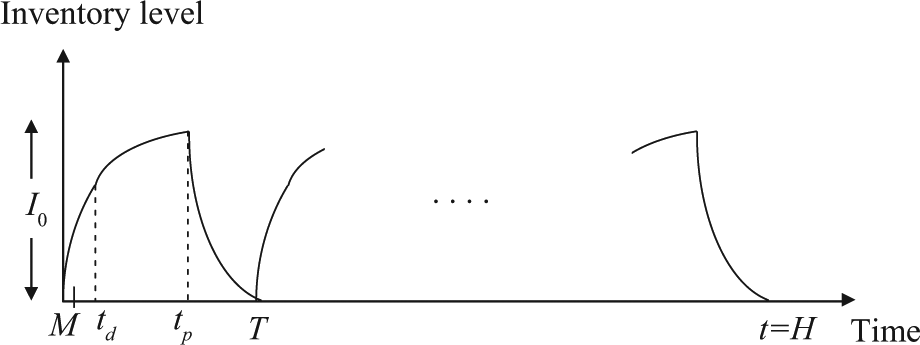
Here, we considered a production inventory system for non-instantaneous deteriorating items, which will be described as follows. During the interval [0, t_d], the inventory level increases due to production as the production rate is much greater than the demand rate. At time t_d, deterioration starts, and thus, the inventory level increases due to the production rate which is greater than the demand and the deterioration until the maximum inventory level is reached at t = t_p. During the interval [t_p, T], there is no production and the inventory level decreases due to demand and deterioration until the inventory level becomes 0 at t = T. The graphical representation of the model is shown in Figure 1. In this illustration, the demand rate increases exponentially with time (i.e. λ > 0).

Figure 1.

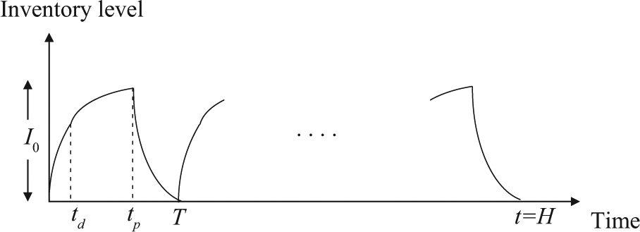
Graphical representation of an inventory system.

During the time interval [0, t_d], the system is subject to the effect of production and demand. Therefore, the change of the inventory level at time t, I₁(t) is governed by

\frac{d I_{1} (t)}{dt} = R - D (t, p)

(1)

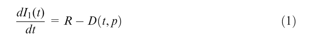
With the condition I₁(0) = 0, solving equation (1) yields

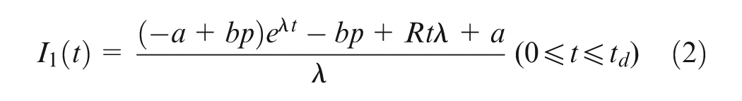
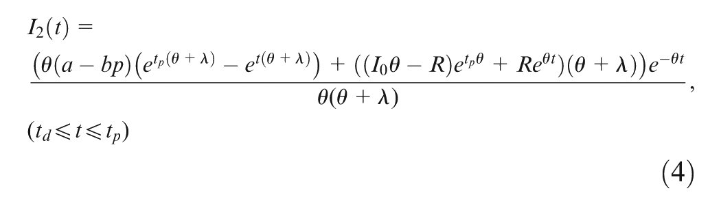
I_{1} (t) = \frac{(- a + bp) e^{λ t} - bp + Rt λ + a}{λ} (0 \leq t \leq t_{d})

(2)

In the time interval [t_d, t_p], the system is affected by the combination of the production, demand, and deterioration. Hence, the change of the inventory level at time t, I₂(t), is governed with

\frac{d I_{2} (t)}{dt} + θ I_{2} (t) = R - D (t, p)

(3)

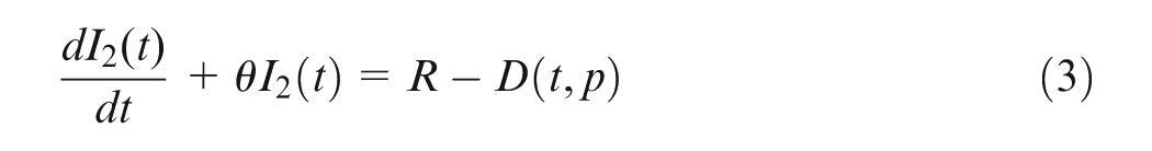
With the condition $I_{2} (t_{p}) = I_{0}$ , equation (3) yields

\begin{matrix} I_{2} (t) = \\ \frac{(θ (a - bp) (e^{t_{p} (θ + λ)} - e^{t (θ + λ)}) + ((I_{0} θ - R) e^{t_{p} θ} + R e^{θ t}) (θ + λ)) e^{- θ t}}{θ (θ + λ)}, \\ (t_{d} \leq t \leq t_{p}) \end{matrix}

(4)

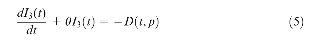
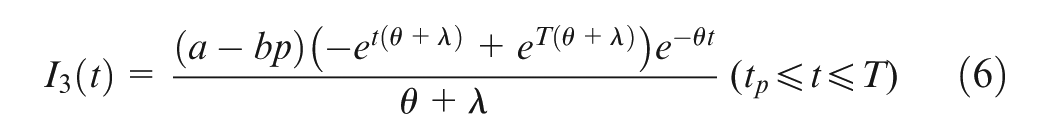
In the third interval [t_p, T], the inventory level decreases due to demand and deterioration. Thus, the differential equation below represents the inventory status

\frac{d I_{3} (t)}{dt} + θ I_{3} (t) = - D (t, p)

(5)

By the condition $I_{3} (T) = 0$ , the solution of equation (5) is

I_{3} (t) = \frac{(a - bp) (- e^{t (θ + λ)} + e^{T (θ + λ)}) e^{- θ t}}{θ + λ} (t_{p} \leq t \leq T)

(6)

Furthermore, in this interval with the condition $I_{3} (t_{p}) = I_{0}$ , the maximum inventory level (I₀) yields the following value

I_{0} = \frac{(a - bp) (- e^{t_{p} (θ + λ)} + e^{T (θ + λ)}) e^{- θ t_{p}}}{θ + λ}

(7)

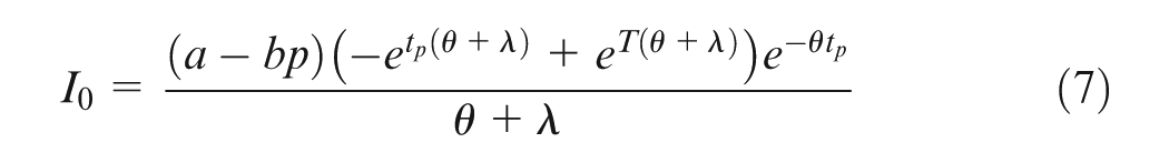
Note that the production occurs in continuous time-spans [0, t_p]. Hence, the lot size in this problem is given by

Q = R \cdot t_{p}

(8)

Now, we can obtain the present value of inventory costs and sales revenue for the first cycle, which consists of the following elements:

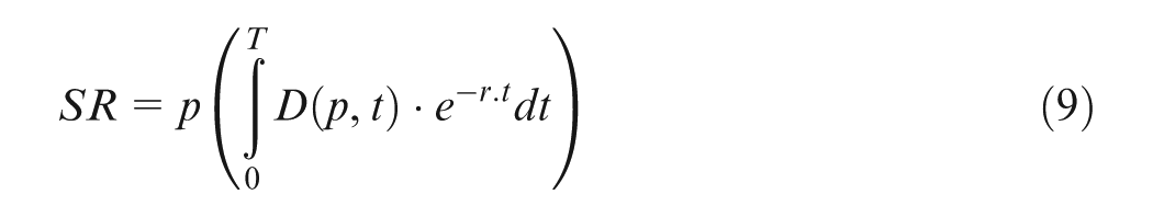
1. SR. The present value of the sales revenue for the first cycle

SR = p (\int_{0}^{T} D (p, t) \cdot e^{- r . t} dt)

(9)

2. PC. The present value of production cost for the first cycle

PC = c_{2} (R \cdot t_{p})

(10)

3. K. Since production setup in each cycle is done at the beginning of each cycle, the present value of setup cost for the first cycle is K, which is a constant value.

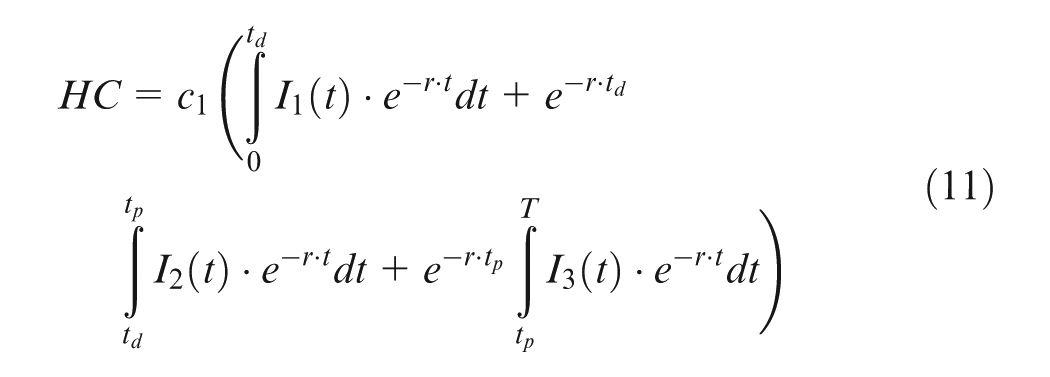
4. HC. The present value of inventory carrying cost for the first cycle

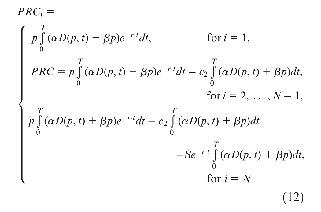
H C = c_{1} (\int_{0}^{t_{d}} I_{1} (t) \cdot e^{- r \cdot t} d t + e^{- r \cdot t_{d}} \int_{t_{d}}^{t_{p}} I_{2} (t) \cdot e^{- r \cdot t} d t + e^{- r \cdot t_{p}} \int_{t_{p}}^{T} I_{3} (t) \cdot e^{- r \cdot t} d t)

(11)

5. The present value of return cost for each cycle.

We assume that returns from period $i - 1$ are available for resale at the beginning of period i (except the first period in which there is no cycle previous to it). Also, it is assumed that the salvage value of the product at the end of the last period (i = N) is S. Therefore, the present value of return cost and resale revenue for each cycle is obtained as follows

\begin{matrix} PR C_{i} = \\ {\begin{matrix} \begin{matrix} p \int_{0}^{T} (α D (p, t) + β p) e^{- r \cdot t} dt, for i = 1, \\ PRC = p \int_{0}^{T} (α D (p, t) + β p) e^{- r \cdot t} dt - c_{2} \int_{0}^{T} (α D (p, t) + β p) dt, \\ for i = 2, \dots, N - 1, \end{matrix} \\ p \int_{0}^{T} (α D (p, t) + β p) e^{- r \cdot t} dt - c_{2} \int_{0}^{T} (α D (p, t) + β p) dt \\ \begin{matrix} - S e^{- r \cdot t} \int_{0}^{T} (α D (p, t) + β p) dt, \\ for i = N \end{matrix} \end{matrix} \end{matrix}

(12)

6. The present value of interest payable for the first cycle.

For each cycle, we need to consider cases where the length of the credit period is longer or shorter than the length of time in which the product exhibits no deterioration (t_d) and the length of the production period (t_p). Thus, we calculate the present value of interest payable for the items kept in stock under the following three cases.

Case 1. The delay time of payments occurs before deteriorating time or 0 < M≤t_d (see Figure 2).

Figure 2.

0 < M≤t_d (case 1).

In this case, payment for items is settled and the retailer starts paying the interest charged for all unsold items in inventory with rate I_p. Thus, the present value of interest payable for the first cycle is given as follows

I P_{1} = c_{2} I_{p} {e^{- r \cdot M} \int_{M}^{t_{d}} I_{1} (t) \cdot e^{- r \cdot t} d t + e^{- r \cdot t_{d}} \int_{t_{d}}^{t_{p}} I_{2} (t) \cdot e^{- r \cdot t} d t + e^{- r \cdot t_{p}} \int_{t_{p}}^{T} I_{3} (t) \cdot e^{- r \cdot t} d t}

(13)

Case 2. The delay time of payments occurs after deteriorating time and before production period time; that is, t_d < M≤t_p (see Figure 3).

Figure 3.

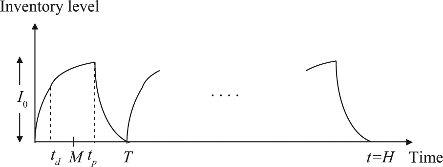
t_d < M≤t_p (case 2).

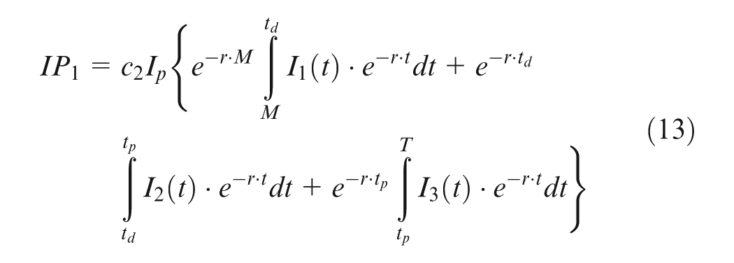
The conditions of this case are similar to those for case 1. Thus, the present value of interest payable for the first cycle is given as follows

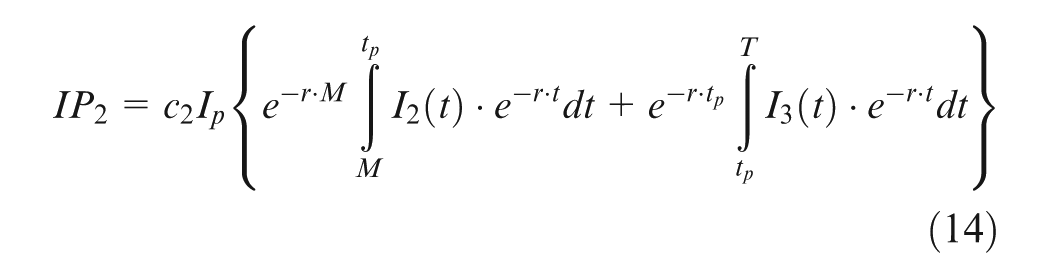
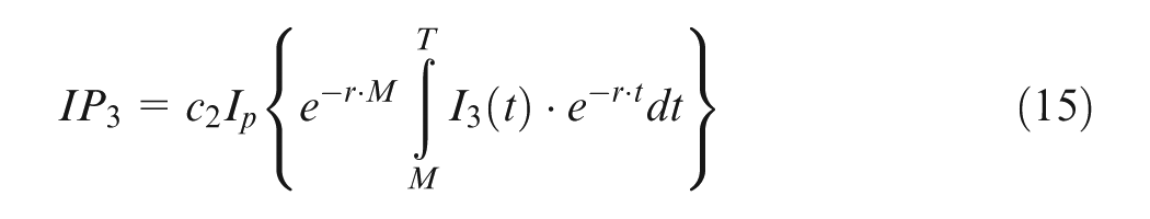
I P_{2} = c_{2} I_{p} {e^{- r \cdot M} \int_{M}^{t_{p}} I_{2} (t) \cdot e^{- r \cdot t} dt + e^{- r \cdot t_{p}} \int_{t_{p}}^{T} I_{3} (t) \cdot e^{- r \cdot t} dt}

(14)

Case 3. The delay time of payments occurs after production period time and before duration of inventory cycle or t_p < M≤T (see Figure 4).

Figure 4.

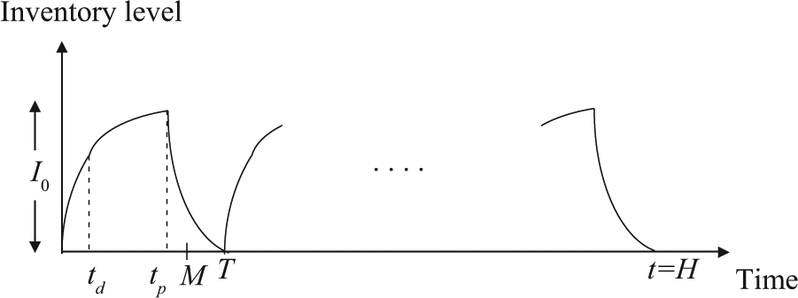
t_p < M≤T (case 3).

In this case, the retailer starts paying the interest for the items in stock from time M to T with rate I_p. Hence, the present value of interest payable for the first cycle is as follows

I P_{3} = c_{2} I_{p} {e^{- r \cdot M} \int_{M}^{T} I_{3} (t) \cdot e^{- r \cdot t} dt}

(15)

7. The present value of interest earned for the first cycle.

There are different ways to tackle the interest earned. Here, we use the approach used in the study by Geetha and Uthayakumar.²¹ We assume that during the time when the account is not settled, the retailer sells the goods and continues to accumulate sales revenue and earns interest with rate I_e. Therefore, the present value of the interest earned for the first cycle is as given below for the three different cases.

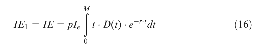
Case 1. The delay time of payments occurs before deteriorating time or 0 < M≤t_d

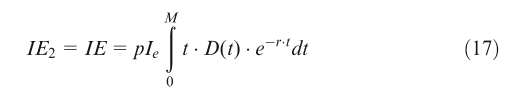
I E_{1} = IE = p I_{e} \int_{0}^{M} t \cdot D (t) \cdot e^{- r \cdot t} dt

(16)

Case 2. The delay time of payments occurs after deteriorating time and before production period time; that is, t_d< M≤t_p

I E_{2} = IE = p I_{e} \int_{0}^{M} t \cdot D (t) \cdot e^{- r \cdot t} dt

(17)

Case 3. The delay time of payments occurs after production period time and before duration of inventory cycle or t_p < M≤T

I E_{3} = IE = p I_{e} \int_{0}^{M} t \cdot D (t) \cdot e^{- r \cdot t} dt

(18)

Consequently, the present value of total profit, denoted by $f (p, t_{p}, N)$ , is given by

f (p, t_{p}, N) = {\begin{matrix} \begin{matrix} \begin{matrix} f_{1} (p, t_{p}, N) = \sum_{i = 0}^{N - 1} (SR - PC - K - HC - PRC + IE - I P_{1}) e^{- r \cdot i \cdot T} \\ + S \cdot e^{- r \cdot H} \int_{0}^{T} (α D (p, t) + β p) dt - c_{2} \int_{0}^{T} (α D (p, t) + β p) dt, \end{matrix} \\ 0 < M \leq t_{d}, \\ f_{2} (p, t_{p}, N) = \sum_{i = 0}^{N - 1} (SR - PC - K - HC - PRC + IE - I P_{2}) e^{- r \cdot i \cdot T} \end{matrix} \\ \begin{matrix} \begin{matrix} + S \cdot e^{- r \cdot H} \int_{0}^{T} (α D (p, t) + β p) dt - c_{2} \int_{0}^{T} (α D (p, t) + β p) dt, \\ t_{d} < M \leq t_{p} \end{matrix} \\ \begin{matrix} f_{3} (p, t_{p}, N) = \sum_{i = 0}^{N - 1} (SR - PC - K - HC - PRC + IE - I P_{3}) e^{- r \cdot i \cdot T} \\ \begin{matrix} + S \cdot e^{- r \cdot H} \int_{0}^{T} (α D (p, t) + β p) dt - c_{2} \int_{0}^{T} (α D (p, t) + β p) dt, \\ t_{p} < M \leq T \end{matrix} \end{matrix} \end{matrix} \end{matrix}

(19)

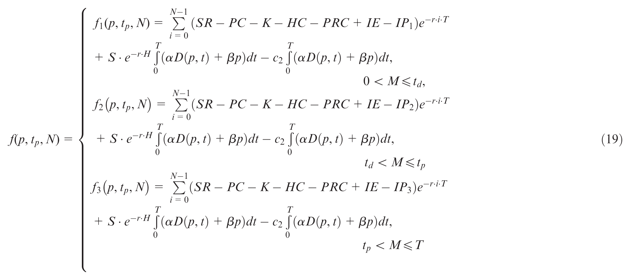
which we want to maximize, subject to the following constraints

p > 0, 0 < t_{p} < T, N \in N

The value of the variable $T$ can be replaced by the equation $T = H / N$ for some constant $H > 0$ , and we will use Maclaurin’s approximation for $\sum_{i = 0}^{N - 1} e^{- r . i . T} ≅ (1 - e^{- r . N . T}) / (1 - e^{- r . T})$ . Thus, the objective of this article is to determine the values of $t_{p}$ , p, and N that maximize $f (p, t_{p}, N)$ subject to $p > 0$ and $0 < t_{p} < T$ , where N is a discrete variable and p and $t_{p}$ are continuous variables. However, since $f (p, t_{p}, N)$ is a very complicated function due to high-power expressions in the exponential function, it is difficult to show analytically the validity of the sufficient conditions. Hence, if more than one local maximum value exists, we would attain the largest of the local maximum values over the regions subject to $p > 0$ and $0 < t_{p} < T$ . The largest value is referred to as the global maximum value of $f (p, t_{p}, N)$ . So far, the procedure is to locate the optimal values of p and $t_{p}$ when N is fixed. Since N is a discrete variable, the following algorithm can be used to determine the optimal values of p, $t_{p}$ , and N.

The optimal solution procedure

The objective function has three variables. The number of production cycles (N) is a discrete variable, and the production period in an inventory cycle (t_p) and the selling price per unit (p) are continuous variables. We use the following algorithm for case 1, 0 < M≤t_d, to obtain the optimal amount of t_p, p, and N.

Step 1. Let $N = 1$ .

Step 2. Take the partial derivatives of $f_{1} (p, t_{p}, N)$ with respect to p and $t_{p}$ , and equate the results to zero; then the necessary conditions for optimality are

\frac{\partial}{\partial p} f_{1} (p, t_{p}, N) = 0

(20)

and

\frac{\partial}{\partial t_{p}} f_{1} (p, t_{p}, N) = 0

(21)

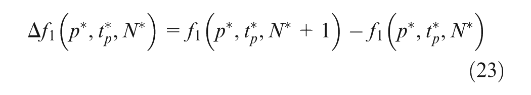
In Appendix 2, we use the formula of $f_{1} (p, t_{p}, N)$ from the first part of equation (19) and insert into equations (20) and (21).

Step 3. For different integer $N$ values, derive $t_{p}^{*}$ and $p^{*}$ from equations (20) and (21). Substitute $(p^{*}, t_{p}^{*}, N^{*})$ into $f_{1} (p, t_{p}, N)$ from the first part of equation (19) to derive $f_{1} (p^{*}, t_{p}^{*}, N^{*})$ .

Step 4. Add one unit to N and repeat steps 2 and 3 for the new N. If there is no increase in the last value of $f_{1} (p, t_{p}, N)$ , then consider the previous one which has the maximum value.

The point $(p^{*}, t_{p}^{*}, N^{*})$ and the value $f_{1} (p^{*}, t_{p}^{*}, N^{*})$ constitute the optimal solution and satisfy the following conditions

Δ f_{1} (p^{*}, t_{p}^{*}, N^{*}) < 0 < Δ f_{1} (p^{*}, t_{p}^{*}, N^{*} - 1)

(22)

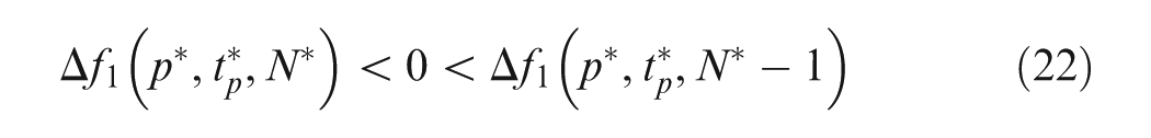
where

Δ f_{1} (p^{*}, t_{p}^{*}, N^{*}) = f_{1} (p^{*}, t_{p}^{*}, N^{*} + 1) - f_{1} (p^{*}, t_{p}^{*}, N^{*})

(23)

We substitute $(p^{*}, t_{p}^{*}, N^{*})$ into equation (8) to derive the Nth production lot size.

If the objective function was strictly concave, the following sufficient conditions must be satisfied

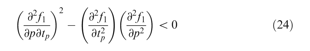
{(\frac{\partial^{2} f_{1}}{\partial p \partial t_{p}})}^{2} - (\frac{\partial^{2} f_{1}}{\partial t_{p}^{2}}) (\frac{\partial^{2} f_{1}}{\partial p^{2}}) < 0

(24)

and any one of the following conditions

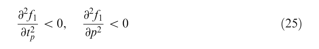
\frac{\partial^{2} f_{1}}{\partial t_{p}^{2}} < 0, \frac{\partial^{2} f_{1}}{\partial p^{2}} < 0

(25)

It is difficult to show the validity of the above sufficient conditions, analytically, due to involvement of a high-power expression of the exponential function. However, it can be assessed numerically in the following example.

A numerical example

To illustrate the solution procedure and the results, let us apply the proposed algorithm to solve the following numerical example. The results can be found by applying Maple 13. This example is based on the following parameters and functions

R = 500 units/unit time, c₁ = US$8/unit/unite time, c₂ = US$10/unit, t_d = 0.04 unit time, K = US$250/production run, σ = 0.08, r = 0.08, a = 200, b = 0.5, λ = −0.02, H = 40 unit time, α = 0.5, β = 0.7, S = US$3/unit, M = 0.02 unit time, I_p = 0.15/US$/unit time, and I_e = 0.12/US$/unit time.

Using the solution procedure described above, the related results are shown in Table 1, and all the given conditions in equations (24) and (25) are satisfied. In this example, the maximum present value of the total profit is found when the number of cycle (N) is 23. With 23 replenishments, the optimal solution is as follows

\begin{matrix} p^{*} & = 56.182, t_{p}^{*} = 1.109, T^{*} = 1.739, \\ f_{1}^{*} & = 3523.379, Q^{*} = 554.934 \end{matrix}

Table 1.

Optimal solution of the example.

N	p	Time interval		Q	f ₁
		t_p	T		f ₁
22	56.243	1.110	1.818	555.384	3497.970
23^a	56.182^a	1.109^a	1.739^a	554.934^a	3523.379^a
24	56.126	1.108^a	1.666	554.469	3468.388

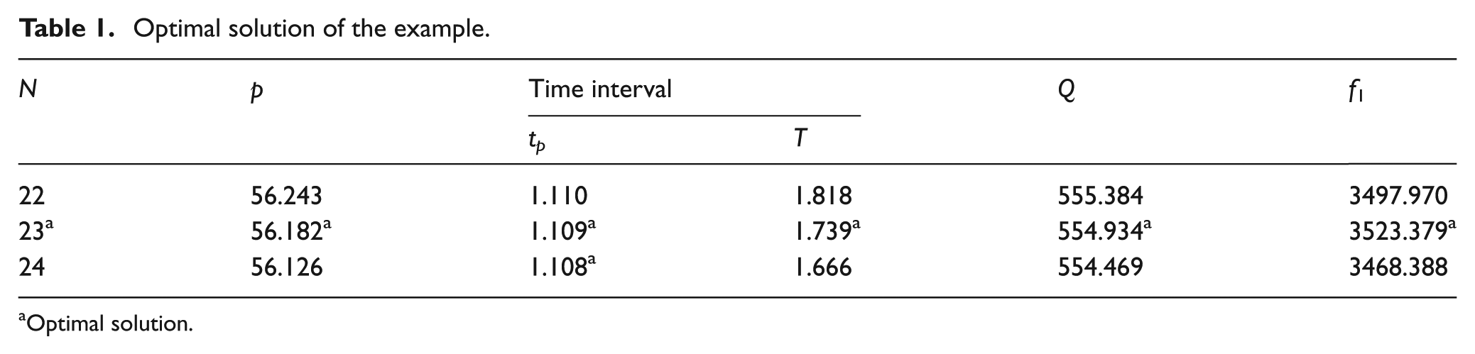
Optimal solution.

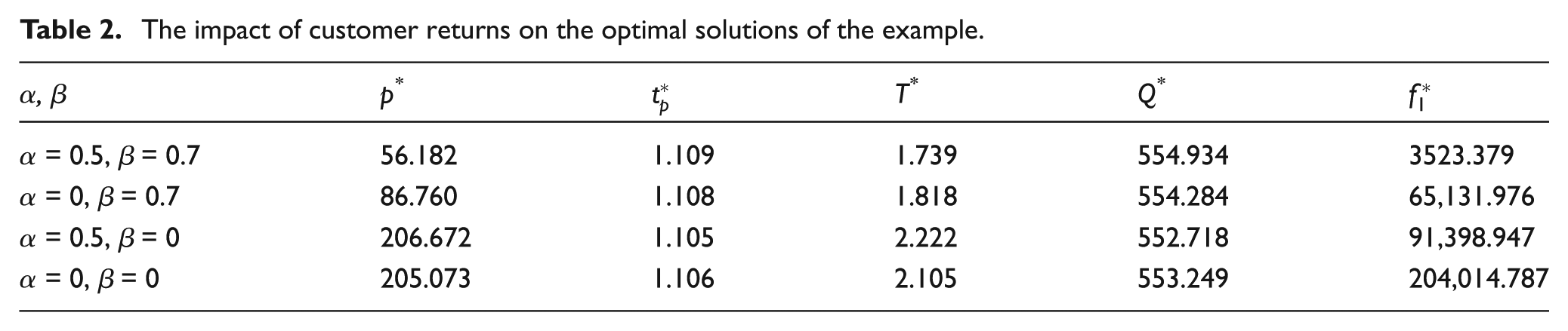
We obtain the results of this example for analyzing the impact of customer returns on the optimal solution and financial performance (Table 2). The results illustrate that when returns are proportional to the quantity sold only (i.e. β= 0), the firm should raise the price and reduce the production quantity, but if returns are proportional to price only (i.e. α= 0), the firm should decrease the price and increase the production quantity. The results confirm that when returns increase with the product price (when production costs are constant), the firm should set a lower price to the no-returns case (in order to discourage returns). Increasing α and/or β reduces the firm’s profit.

Table 2.

The impact of customer returns on the optimal solutions of the example.

α, β	p ^*	$t_{p}^{*}$	T ^*	Q ^*	$f_{1}^{}$*
α = 0.5, β = 0.7	56.182	1.109	1.739	554.934	3523.379
α = 0, β = 0.7	86.760	1.108	1.818	554.284	65,131.976
α = 0.5, β = 0	206.672	1.105	2.222	552.718	91,398.947
α = 0, β = 0	205.073	1.106	2.105	553.249	204,014.787

Table 3

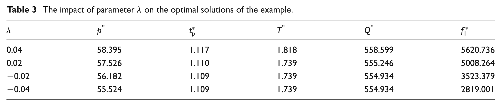
The impact of parameter λ on the optimal solutions of the example.

λ	p ^*	$t_{p}^{*}$	T ^*	Q ^*	$f_{1}^{}$*
0.04	58.395	1.117	1.818	558.599	5620.736
0.02	57.526	1.110	1.739	555.246	5008.264
−0.02	56.182	1.109	1.739	554.934	3523.379
−0.04	55.524	1.109	1.739	554.934	2819.001

Moreover, if we ignored inflation and time value of money (i.e. r = 0), the optimal present value of total profit ( $f_{1}^{*}$ ) is overstated by 24,295.241. The overstatement of profits will lead to the wrong management decision. Therefore, it is important to consider the effects of inflation and the time value of money on inventory policy.

Also, when the supplier does not provide a credit period (i.e. M = 0), the optimal present value of retailer total profit can be found as follows: $f_{1}^{*} = 2930.440$ . It can be seen that the optimal present value of total profit decreases. Thus, retailers should try to get credit periods for their payments if they wish to increase their profit.

Conclusion and outlook

In this article, we study the effects of delay in payments, customer returns, and inflation on joint pricing and inventory control model for an EPQ model with non-instantaneous deteriorating items and price- and time-dependent demand. The customer returns are assumed as a function of price and demand simultaneously. To the best of our knowledge, this is the first model in pricing and inventory control models that considers EPQ model, delay in payments, inflation, non-instantaneously deteriorating items, and time- and price-dependent demand. The mathematical models are derived to determine the optimal selling price, the optimal length of inventory cycle time, and the optimal production quantity simultaneously. An optimization algorithm is presented to derive the optimal decision variables. Finally, a numerical example is solved and the effects of the customer returns, inflation, and delay in payments are also discussed.

The following inferences can be made from the results obtained.

The results of analyzing customer returns provide the following insights (Table 2). A company facing customer returns that depend on the price set for the product could decrease returns by reducing price and increasing the production quantity. On the other hand, when customer returns increase with quantity of product sold, the company could mitigate the loss in profit resulting from the customer returns by increasing the price and decreasing the production quantity. If the quantity of returns depends on the price and quantity sold simultaneously, the company could set a higher or lower price based on dominant returns form.

It can be seen that there is an improvement in the optimal present value of total profit when the discount rate of inflation is ignored (i.e. r = 0). The overstatement of profits will lead to the wrong management decision. Therefore, it is important to consider the effects of inflation and the time value of money on inventory policy.

The results show that when a delay in payments is allowed, the optimal present value of total profit for the retailer does enhance. Thus, retailers should try to get credit periods for their payments if they wish to increase their profit.

The proposed model can be extended in numerous ways for future research. For example, we could incorporate (1) stochastic demand function, (2) two warehouse, (3) quantity discount, (4) deteriorating cost, and (5) shortages.

Footnotes

Appendix 1

Appendix 2

For a given value of N, the necessary conditions for finding the optimal values of $p^{*}$ and $t_{p}^{*}$ are given as follows

\begin{matrix} \frac{\partial}{\partial p} f_{1} (p, t_{p}, N) \\ = - \frac{1}{{(- λ + r)}^{2} (θ + λ) cr (σ + λ) (θ + r) λ (- 1 + e^{- \frac{rH}{N}})} ((- rb λ c_{1} e^{- r t_{d}} e^{(- r - σ) t_{p} - r t_{d}} (θ + λ) \\ {(- λ + r)}^{2} (θ + r) e^{\frac{((- t_{d} + t_{p}) σ + r t_{p}) N + (σ + λ) H}{N}} \\ - rb λ c_{1} e^{- \frac{rH}{N}} e^{- r t_{p}} (θ + λ) {(- λ + r)}^{2} (θ + r) e^{\frac{(σ + λ + r) H - N t_{p} (r + σ)}{N}} \\ + rb e^{- \frac{rH}{N}} e^{- r t_{p}} c_{1} λ (θ + λ) (- λ + r) (θ + r) (σ + r) e^{\frac{- t_{p} (- λ + r) N + rH}{N}} \\ + rb λ c_{1} e^{- r t_{d}} e^{(- r - σ) t_{p} - r t_{d}} (θ + λ) {(- λ + r)}^{2} (θ + r) e^{\frac{(σ + λ) H - r t_{d} N}{N}} \\ - rb λ c_{2} I_{p} e^{- r t_{p}} (σ + λ) {(- λ + r)}^{2} (σ + r) e^{- (- r - θ) t_{p} + (θ + λ) T} \\ - rb λ c_{2} I_{p} e^{- r t_{d}} e^{- (- r - θ) t_{p} - r t_{d}} (σ + λ) {(- λ + r)}^{2} (σ + r) e^{(t_{p} - t_{d} + T) θ + T λ + r t_{p}} \\ - rb λ c_{1} e^{- r t_{d}} (θ + λ) (- λ + r) (θ + r) (e^{(σ + λ) t_{p} + r t_{d}} - e^{(σ + r) t_{p} + λ t_{d}}) (r + σ) e^{(- σ - r) t_{p} - r t_{d}} \\ + (λ ((- r - θ) e^{(θ + λ) t_{p} + r t_{d}} + (θ + r) e^{(θ + r) t_{p} + λ t_{d}} \\ + e^{(θ + λ) T + r t_{d}} (- λ + r)) e^{- r t_{d}} (- λ + r) (σ + r) c_{2} r I_{p} b e^{(- θ - r) t_{p} - r t_{d}} \\ + r (θ + λ) λ (- λ + r) (θ + r) (σ + r) (- 2 bp + a) e^{- \frac{H (- λ + r)}{N}} λ (- λ + r) (θ + λ) \\ (((- 2 (- \frac{1}{2} c_{2} + p) α b - β c_{2} + 2 p β + a α) r - 2 β (- \frac{1}{2} c_{2} + p) λ) \\ (σ + r) e^{\frac{rH}{N}} - (c_{1} be -^{r t_{p}} + α (r + σ) ((- 2 p + c_{2}) b + a)) re \frac{λ H}{N} \\ - 2 (- λ + r) β (- \frac{1}{2} c_{2} + p) (r + σ)) (θ + r) e^{\frac{rH}{N}} \\ + (r + θ) (r I_{e} λ (θ + λ) (θ + r) (- 2 bp + a) (rM - λ M + 1) e^{- M (- λ + r)}) \\ + rb λ e^{- r t_{p}} I_{p} c_{2} (- λ + r) e^{- T (- λ + r)} + rb e^{- r (M + t_{d})} e^{- rM} c_{2} (- λ + r) e^{rM + λ t_{d}} \\ - rb e^{- r (M + t_{d})} e^{- rM} I_{p} c_{2} (- λ + r) e^{r t_{d} + λ M} \\ - c_{2} b I_{p} e^{- rM} {(- λ + r)}^{2} (- e^{r t_{d}} + e^{rM}) e^{- r (M + t_{d})} \\ + b c_{1} (- λ + r) (- r + r e^{λ t_{d}} + λ - e^{r t_{d}} λ) e^{- r t_{d}} \\ + r λ (- λ + r + I_{e}) (- 2 bp + a)) (θ + r)))) (σ + λ)) (- 1 + e^{- rH})) \\ + \frac{S e^{- rH} (α Nb - α e \frac{H λ}{N} Nb + β H λ}{λ N} - \frac{c_{2} (α Nb - α e \frac{H λ}{N} Nb + β H λ}{λ N} = 0 \end{matrix}

and

\begin{array}{l} \frac{\partial}{\partial t_{p}} f_{1} (p, t_{p}, N) \\ = \frac{1}{(σ + λ) (- λ + r) (θ + r) (σ + r) (θ + λ) (- 1 + e^{- \frac{r H}{N}})} ((- 1 + e^{- r H}) (- 2 (r + \frac{1}{2} σ) \\ (a - b p) (- λ + r) (θ + r) e^{- r t_{p}} e^{- \frac{r H}{N}} (θ + λ) c_{1} e^{- \frac{H (σ + λ + r) - N t_{p} (σ + r)}{N}} \\ + 2 (- \frac{1}{2} λ + r) (a - b p) (θ + r) e^{- r t_{p}} (σ + r) e^{- \frac{r H}{N}} (θ + λ) c_{1} e^{\frac{- t_{p} (- λ + r) N + r H}{N}} \\ + c_{1} e^{- r t_{d}} e^{(- σ - r) t_{p} - r t_{d}} (θ + λ) (- λ + r) (θ + r) (σ + r) (a - b p) e^{- \frac{H (σ + λ) + N t_{d} r}{N}} \\ + (- λ + r) e^{- r t_{d}} (θ + r) (- R (σ + λ) e^{(2 σ + r) t_{p} - σ t_{d}} - (σ + r) (a - b p) e^{(σ + λ) t_{p} + r t_{d}} + R e^{r t_{d} + σ t_{p}} (σ + λ)) (θ + λ) c_{1} e^{(- σ - r) t_{p} - r t_{d}} \\ + (σ + λ) (c_{2} (- λ + r) I_{p} e^{- r t_{d}} (σ + r) (- R (θ + λ) e^{(2 θ + r) t_{p} - θ t_{d}} - (θ + r) (a - b p) e^{(θ + λ) t_{p} + r t_{d}} + (θ + r) (a - b p) e^{(θ + λ) T + r t_{d}} + R e^{r t_{d} + θ t_{p}} (θ + λ)) e^{(- θ - r) t_{p} - r t_{d}} - r e^{\frac{λ H}{N}} e^{- r t_{p}} c_{1} (θ + λ) (θ + r) (a - b p) e^{- \frac{r H}{N}} + c_{2} (σ + r)) \\ (2 (- \frac{1}{2} λ + r) (a - b p) I_{p} (θ + r) e^{- r t_{p}} e^{- t_{p} (- λ + r)} + (- r e^{- r t_{p}} I_{p} (a - b p) e^{- T (- λ + r)} + R (- λ + r) (θ + r) (θ + λ)))) = 0 \end{array}

Declaration of conflicting interests

The authors declare that there is no conflict of interest.

Funding

This research received no specific grant from any funding agency in the public, commercial, or not-for-profit sectors.

References

Ghare

Schrader

. A model for exponentially decaying inventory system. Int J Prod Res 1963; 21: 449–460.

Covert

Philip

. An EOQ model for items with Weibull distribution deterioration. AIIE T 1973; 5: 323–326.

Hariga

. Optimal EOQ models for deteriorating items with time-varying demand. J Oper Res Soc 1996; 47: 1228–1246.

Heng

Labban

Linn

. An order-level lot-size inventory model for deteriorating items with finite replenishment rate. Comput Ind Eng 1991; 20: 187–197.

Jaggi

Aggarwal

Goel

. Optimal order policy for deteriorating items with inflation induced demand. Int J Prod Econ 2006; 103: 707–714.

Moon

Giri

. Economic order quantity models for ameliorating/deteriorating items under inflation and time discounting. Eur J Oper Res 2005; 162: 773–785.

Sarker

Mukherjee

Balan

. An order-level lot size inventory model with inventory-level dependent demand and deterioration. Int J Prod Econ 1997; 48: 227–236.

Wee

. A deterministic lot-size inventory model for deteriorating items with shortages and a declining market. Comput Oper Res 1995; 22: 345–356.

Goyal

Giri

. Recent trends in modeling of deteriorating inventory. Eur J Oper Res 2001; 134: 1–16.

10.

Shi

Zhang

Lai

. Optimal ordering and pricing policy with supplier quantity discounts and price-dependent stochastic demand. Optimization 2012; 61: 151–162.

11.

Dye

. Joint pricing and ordering policy for a deteriorating inventory with partial backlogging. Omega 2007; 35: 184–189.

12.

Abad

. Optimal price and order size for a reseller under partial backordering. Comput Oper Res 2001; 28: 53–65.

13.

Dye

Quyang

Hsieh

. Inventory and pricing strategy for deteriorating items with shortages: a discounted cash flow approach. Comput Ind Eng 2007; 52: 29–40.

14.

Chang

Teng

Ouyang

. Retailer’s optimal pricing and lot-sizing policies for deteriorating items with partial backlogging. Eur J Oper Res 2006; 168: 51–64.

15.

Samadi

Mirzazadeh

Pedram

. Fuzzy pricing, marketing and service planning in a fuzzy inventory model: a geometric programming approach. Appl Math Model 2013; 37: 6683–6694.

16.

Tsao

Sheen

. Dynamic pricing, promotion and replenishment policies for a deteriorating item under permissible delay in payments. Comput Oper Res 2008; 35: 3562–3580.

17.

Ouyang

Yang

. An optimal replenishment policy for non-instantaneous deteriorating items with stock dependent demand and partial backlogging. Int J Prod Econ 2006; 101: 369–384.

18.

Ouyang

Yang

. A study on an inventory model for non-instantaneous deteriorating items with permissible delay in payments. Comput Ind Eng 2006; 51: 637–651.

19.

Chang

Teng

Goyal

. Optimal replenishment policies for non instantaneous deteriorating items with stock-dependent demand. Int J Prod Econ 2010; 123: 62–68.

20.

Yang

Ouyang

. Retailers optimal pricing and ordering policies for non-instantaneous deteriorating items with price-dependent demand and partial backlogging. Math Probl Eng 2009; 2009: ID 198305.

21.

Geetha

Uthayakumar

. Economic design of an inventory policy for non-instantaneous deteriorating items under permissible delay in payments. J Comput Appl Math 2010; 223: 2492–2505.

22.

Musa

Sani

. Inventory ordering policies of delayed deteriorating items under permissible delay in payments. Int J Prod Econ 2012; 136(1): 75–83.

23.

Maihami

Nakhai Kamalabadi

. Joint pricing and inventory control for non-instantaneous deteriorating items with partial backlogging and time and price dependent demand. Int J Prod Econ 2012; 136: 116–122.

24.

Maihami

Nakhai Kamalabadi

. Joint control of inventory and its pricing for non-instantaneously deteriorating items under permissible delay in payments and partial backlogging. Math Comput Model 2012; 55: 1722–1733.

25.

Buzacott

. Economic order quantities with inflation. Oper Res Quart 1975; 26: 553–558.

26.

Misra

. A note on optimal inventory management under inflation. Nav Res Logist Q 1979; 26: 161–165.

27.

Park

. Inflationary effect on EOQ under trade-credit financing. Int J Pol Inform 1986; 10: 65–69.

28.

Datta

Pal

. Effects of inflation and time value of money on an inventory model with linear time-dependent demand rate and shortages. Eur J Oper Res 1991; 52: 326–333.

29.

Goal

Gupta

Bector

. Impact of inflation on economic quantity discount schedules to increase vendor profits. Int J Syst Sci 1991; 22: 197–207.

30.

Hall

. Price changes and order quantities: impacts of discount rate and storage costs. IIE Trans 1992; 24: 104–110.

31.

Sarker

Pan

. Effects of inflation and time value of money on order quantity and allowable shortage. Int J Prod Econ 1994; 34: 65–72.

32.

Hariga

Ben-Daya

. Optimal time varying lot-sizing models under inflationary conditions. Eur J Oper Res 1996; 89: 313–325.

33.

Horowitz

. EOQ and inflation uncertainty. Int J Prod Econ 2000; 65: 217–224.

34.

Moon

Lee

. The effects of inflation and time value of money on an economic order quantity with a random product life cycle. Eur J Oper Res 2000; 125: 558–601.

35.

Mirzazadeh

Seyed-Esfehani

Fatemi-Ghomi

SMT

. An inventory model under uncertain inflationary conditions, finite production rate and inflation-dependent demand rate for deteriorating items with shortages. Int J Syst Sci 2009; 40: 21–31.

36.

Sarkar

Moon

. An EPQ model with inflation in an imperfect production system. Appl Math Comput 2011; 217(13): 6159–6167.

37.

Sarkar

Sana

Chaudhuri

. An imperfect production process for time varying demand with inflation and time value of money—an EMQ model. Expert Syst Appl 2011; 38(15): 13543–13548.

38.

Taheri-Tolgari

Mirzazadeh

Jolai

. An inventory model for imperfect items under inflationary conditions with considering inspection errors. Comput Math Appl 2012; 63: 1007–1019.

39.

Gholami-Qadikolaei

Mirzazadeh

Tavakkoli-Moghaddam

. A stochastic multiobjective multiconstraint inventory model under inflationary condition and different inspection scenarios. Proc IMechE, Part B: J Engineering Manufacture 2013; 227(7): 1057–1074.

40.

Wee

Law

. Replenishment and pricing policy for deteriorating items taking into account the time value of money. Int J Prod Econ 2001; 71: 213–220.

41.

Hsieh

Dye

. Pricing and lot-sizing policies for deteriorating items with partial backlogging under inflation. Expert Syst Appl 2010; 37: 7234–7242.

42.

Hou

Lin

. Optimal pricing and ordering policies for deteriorating items with multivariate demand under trade credit and inflation. Opsearch 2013; 50: 404–417.

43.

Ghoreishi

Arshsadi-Khamseh

Mirzazadeh

. Joint optimal pricing and inventory control for deteriorating items under inflation and customer returns. J Ind Engineering 2013; 2013: ID 709083.

44.

Ghoreishi

Mirzazadeh

Weber

. Optimal pricing and ordering policy for non-instantaneous deteriorating items under inflation and customer returns. Optimization. Epub ahead of print 18November2013. DOI: 10.1080/02331934.2013.853059.

45.

Hess

Mayhew

. Modeling merchandise returns in direct marketing. J Direct Mark 1997; 11: 20–35.

46.

Anderson

Hansen

Simister

. How are demand and returns related?Theory and empirical evidence. Working paper, Kellogg School of Management, Northwestern University, Evanston, IL, February 2006.

47.

Chen

Bell

. The impact of customer returns on pricing and order decisions. Eur J Oper Res 2009; 195: 280–295.

48.

Zhu

. Joint pricing and inventory replenishment decisions with returns and expediting. Eur J Oper Res 2012; 216: 105–112.

Optimal pricing and lot-sizing policies for an economic production quantity model with non-instantaneous deteriorating items,permissible delay in payments,customer returns,and inflation

Abstract

Keywords

Introduction

Analysis method and assumptions

Analysis method

Assumptions

The model formulation

The optimal solution procedure

A numerical example

Conclusion and outlook

Footnotes

Appendix 1

Appendix 2

Declaration of conflicting interests

Funding

References