
Abstract
This article presents inspection scenarios for the multiobjective multiconstraint mixed backorder and lost sales inventory model with imperfect items in which the order quantity, reorder point, ordering cost, lead time, and backorder rate are decision variables. The objectives are minimizing expected annual cost and variance of shortages. The number of imperfect items is assumed to be a beta-binomial random variable. There are two inspection scenarios: the imperfect items observed during inspection and screenings are either all reworked or all discarded. In order to fit some real environment, this study assumes the maximum permissible storage space and available budget are limited. Backorder rate is considered as a function of expected shortages at the end of cycle. Stochastic inflationary conditions with a probability density function are also considered in the presented model. This study assumes that the purchasing cost is paid when an order arrives at the beginning of the cycle, and the ordering cost is paid at the time of the order placing. The aggregate demand follows a normal distribution function. Finally, a solution procedure is proposed in order to solve the discussed multiobjective model. In addition, a numerical example is presented to illustrate the multiobjective model and its solution procedure for different inspection scenarios, and a sensitivity analysis is conducted with respect to the important system parameters.
Introduction
The effect of inflation and time value of money are vital in practical environment. Analysis of inventory system under inflationary condition is carried out using two procedures. The first one determines optimal values of the control variables by minimizing the average annual cost, and the second one determines the optimal ordering policy by minimizing the discounted value of all future costs. Hadley 1 showed that the detailed computations in the simplest case, corresponding to the familiar deterministic lot size model, and the ordering quantities computed by minimizing the average annual cost and by minimizing the discounted cost do not differ significantly. Mirzazadeh 2 extends Hadely’s work by minimizing the inflation and time value of money under uncertain conditions, shortages and the effects of deterioration. The above-mentioned system is formulated with two methods, which are derived under some assumptions that the objective of inventory management is to minimize the average annual cost and the discounted cost. These methods are compared to each other carefully. The results reveal that the mentioned methods (the average annual cost and the discounted cost) have a negligible difference to each other. This study determines optimal values by minimizing the average annual cost under an uncertain inflationary condition.
A number of articles have considered the effect of inflation on the inventory system since 1975. Buzacott 3 dealt with an economic order quantity (EOQ) model with inflation subjects to different types of pricing policies. Misra 4 developed a discounted cost model and included internal (company) and external (general economy) inflation rates for various costs associated with an inventory system. Sarker and Pan 5 surveyed the effects of inflation and the time value of money on an order quantity with a finite replenishment rate. Some efforts were extended to consider variable demands, such as Uthayakumar and Geetha, 6 Vrat and Padmanabhan, 7 Datta and Pal, 8 Hariga, 9 Hariga and Ben-Daya, 10 and Chaung. 11 Roy et al. 12 prepared an inventory model for a deteriorating item with displayed stock-dependent demand under fuzzy inflation and time discounting over a random planning horizon. Mirzazadeh et al. 13 considered stochastic inflationary conditions with variable probability density functions (pdfs) over the time horizon, and the demand rate is dependent on inflation rates. The developed model also implicates to a finite replenishment rate and a finite time horizon with shortage. The objective is to minimize the expected present value of costs over the time horizon. Another research has been performed by Ameli et al. 14 considering an EOQ model for imperfect items under fuzzy inflationary conditions. In addition, Taheri-Tolgari et al. 15 presented a discounted cash-flow approach for an inventory model for imperfect item with considering inspection errors.
A lot of inventory models have been considered under the assumption that shortages are allowed. One important group of these models considers that all customers wait until the arrival of the next replenishment (i.e. full backlogging case) when there is shortage. Another situation is to admit that all the served customers leave the system (i.e. lost sale case). However, in many practical situations, there are customers (i.e. whose needs are not critical at that time) willing to wait for the next replenishment in order to satisfy their demands, while others do not want to or cannot wait and leave the system. These situations are modeled by considering partial backlogging in the information of mathematical models. Some studies16,17 have considered backorder rate as a fixed constant. Some other authors have considered a backorder rate as a function of an expected shortage quantity at the end of the cycle. Their studies are based upon this assumption that the larger amount of the expected shortage at the end of cycle, the smaller amount of customer can wait and hence the smaller backorder rate would be. Ouyang and Chaung 18 were first to introduce this assumption in their model and some other authors generalized this assumption in their models for a backorder rate.19 –22
For the traditional inventory model, lead time is treated as a predetermined constant or a random variable (therefore, it is uncontrollable). Recently, inventory models considering lead time as a decision variable and can be decomposed into several components, each having a crashing cost function for the respective reduced lead time. Liao and Shyu 23 have initiated a study on lead time reduction by presenting an inventory model in which lead time is a decision variable and the order quantity is predetermined. Ben-Daya and Rauf 24 developed a model that considered both lead time and order quantity as decision variables. Moon and Gallego 25 assumed unfavorable lead time demand distribution and solved both continuous review and periodic review models with a mixture of backorders and lost sales using minimax distribution free approach. Ouyang et al. 26 have generalized Ben-Daya and Rauf 24 model in which the lead time demand is considered a normal distribution or distribution free. Later, Hariga and Ben-Daya 16 extend Ouyang et al.’s 26 study and presented both continuous review and periodic review inventory models in partial and perfect lead time demand distribution information environment in which reorder point is treated as a variable. Lee 19 considered an inventory model involving variable lead time with the mixture of distribution. Gholami-Qadikolaei et al. 27 considered an inventory problem with variable lead time, defective items and controllable backorder rate in which a nonlinear relationship exists between the crashing cost and lead time. They calculated optimal reorder point in their study, whereas the previous researchers do not obtain optimal safety factor when they consider backorder rate as a function of expected shortage quantity at the end of cycle in their studies. On the other hand, accompanying the growth of Just-In-Time (JIT) production, which has evidence that many benefits can be obtained from reducing setup cost, the issue of investment in setup cost reduction has received a great deal of attention. Porteus 28 first introduced a framework of the setup cost reduction in the classical EOQ, and then, many authors such as Billington, 29 Kim and Haya, 30 Paknejad et al. 31 and Sarker and Coates 32 have explored the more investigations in this area. Wu and Lin 33 studied on lead time and ordering cost reduction when the receiving quantity is different from the ordered quantity. Lee et al. 21 considered an inventory model with backorder discount and ordering cost reduction including mixture of distribution. Wu and Ouyang 34 examined the effect of defective items on a mixture of backorders and lost sales inventory models, and using the result of a basic theorem from renewal reward processes, 35 they calculated expected annual cost (EAC). Annadurai and Uthayakumar 36 considered an inventory model combining ordering cost and lead time reduction with defective units. Moreover, Ben-Daya and Noman 37 proposed integrated inventory models for inspection policies in which order quantity and reorder point are decision variables.
Recently, Salameh and Jaber 38 proposed an EOQ for a buyer who receives imperfect lots. They extended the traditional EOQ model by accounting for imperfect quality items under the following assumptions: (1) a lot contains a probabilistic fraction of defective items that is independent of lot size and (2) screening rate is finite and it is more than demand rate. Maddah and Jaber 39 proposed an inventory model in which expected annual profit could be calculated using the renewal reward theorem. Khan et al. 40 extended the study by Salameh and Jaber 38 by assuming that stock outs (which are treated as both lost sales and backorders) may occur when screening rate is slower than demand rate. In the case of considering defective units in an order lot, our model formulation differs from the three mentioned articles since the number of defective items is assumed to be a beta-binomial random variable and inspection time is negligible.
There are some inventory models with shortages including restrictions on inventory investment, storage space, or reorder workload. Brown and Gerson 41 proposed some models for stochastic inventory system with the limitation on total inventory investment. Schrady and Choe 42 proposed a model with the total time weighted shortages with limitations on inventory investment and reorder workload. Gardner 43 develops models for minimizing expected approximate backordered sales with the restrictions on aggregate investment and replenishment workload. Schroeder 44 presents a model constrained by total expected annual ordering with an objective of minimizing the expected number of units backordered per year. Hariga 45 presented a stochastic full backlogging inventory system with space restriction in which the order quantity and reorder point are decision variables. Xu and Leung 46 propose an analytical model in a two-party vendor-managed system where the retailer restricts the maximum space allocated to the vendor. Bera et al. 47 presented a minimax distribution free procedure for stochastic lead time and demand inventory model under budget restriction when the purchasing cost payment is due at the time of order receiving in which order quantity and reorder point are decision variables. Moon et al. 48 proposed three extended models with variable capacity. First, they presented an EOQ model with random yields. Second, they developed a multiitem EOQ model with storage space and investment constraint and solved model with Lagrange multiplier method. Third, they applied a distribution free approach to the (Q,r) with variable capacity.
With today’s high inflation rate, it is important to take into account the effect of inflationary condition in the stochastic inventory system. Also, the cost of land acquisition is high in most of the countries, and one of the main concerns of inventory managers is to ensure that storage space is enough when an order arrives. Besides, in order to fit some real and practical environment, the amount received is assumed to be a random variable due to rejection during inspection. So, in the case of controllable lead time, this article, with considering several constraints on the stochastic inventory system, will support managers in decision making (DM).
This study proposes multiobjective stochastic mixed backorder and lost sale continuous review inventory model in which the order quantity, reorder point, lead time, ordering cost, and backordering rate are decision variables. The objectives are minimizing total EAC and variance of shortages. An average annual cost method with stochastic inflationary conditions and pdf is considered in the presented model. The storage space and the budget constraints are also considered in the presented model. Both constraints are random variables since X (i.e. lead time demand) and Y (i.e. number of defective units) are random variables. A chance-constrained programming technique is applied to make the random constraints crisp. This article considers the amount received as random variables due to rejection during inspection. Imperfect units are assumed to be beta-binomial random variable. Different inspection scenarios are assumed including the case when imperfect items are reworked and the case when imperfect items are discarded without reworking. The scenario adopted is the one leading to least overall cost. The piece-wise linear crashing cost function is considered, which is widely used in project management in which the duration of some activities can be reduced by assigning more resources to the activities. The demand for ith source is independent and identically distributed (IID) and normally distributed, and hence, the lead time demand follows a normal distribution function. A solution procedure is proposed to find effective solution of the respective multiconstraint multiobjective inventory model for different inspection scenarios. In addition, a numerical example is presented to illustrate the multiobjective model and its solution procedure for different inspection scenarios, and a sensitivity analysis is conducted with respect to the important system parameters.
This article is organized as follows: In section “Assumptions,” assumptions are given. In section “Inventory inspection model formulation,” we present a mathematical model and explain about two inventory inspection models, in which inflationary condition is not considered. In section “Inventory inspection models with inflation,” we present a mathematical model of two inventory inspection approaches, in which inflationary condition is considered. Solution method is proposed in section “Solution method.” In section “Numerical example,” a numerical example is provided to illustrate the models. Finally, we conclude this article.
Assumptions
The developed model is based on the following assumptions.
Shortages are allowed and partially backlogged.
Inventory position is continuously monitored, and order of size Q is made whenever the inventory level hits the reorder point
The purchasing cost is paid when order arrives (at the beginning of the cycle).
Ordering cost is paid at the time an order is placed.
Shortage cost is calculated at the end of cycle.
The demand rate at the ith source,
where
Lead time demand
The reorder point
Backordering rate is dependent on expected shortage quantity with a negative exponential function as given as follows
Units are demanded in small quantities, so that overshooting of the reorder point is not appreciable.
An arrival order may contain some defective items. The number of defective items in an arriving order of size
Shortage cost does not depend on time.
Planning horizon is infinite.
X (i.e. lead time demand), Y (i.e. number of defective items), and I (i.e. inflation rate) are independent.
The inflation rate is a random variable with a known distribution function.
The cost equations are approximations because inventory levels and demands are treated as continuous instead of discrete quantities.
The time the system is out of stock during a cycle is small compared to the cycle length.
There are no orders outstanding at the time the reorder point is reached.
The reorder level is larger than the mean of the lead time demand.
Inspection is error free and inspection time is negligible.
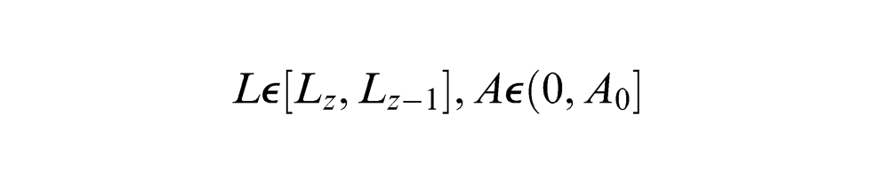
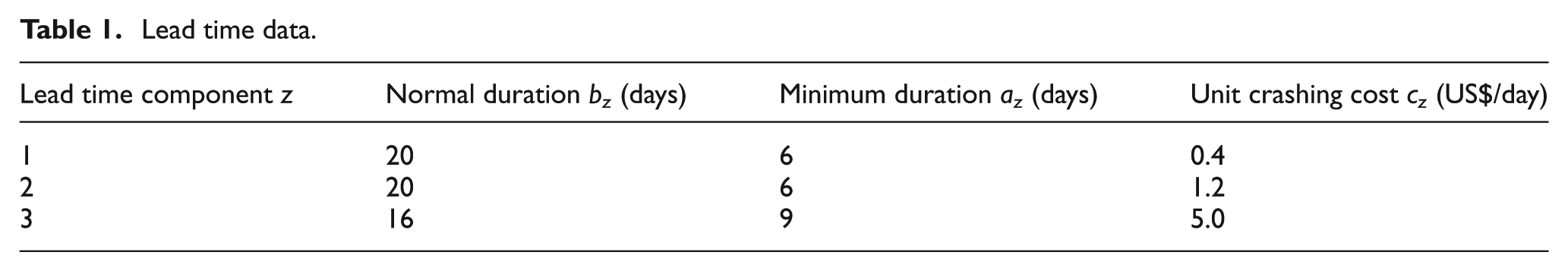
The lead time consists of m mutually independent components. The zth component has a minimum duration
If we let
The components of lead time are crashed one at a time starting with component 1 (because it has a minimum unit crashing cost) and then component 2 and so on.
Inventory inspection model formulation
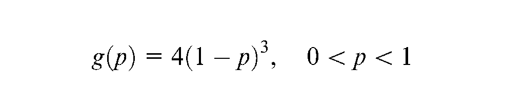
It is considered that defective rate, p, follows a beta-distribution with probability distribution function,
Inspection model without reworking imperfect units
The inventory level of an item will be diminished due to the random demand. The management places an order with the amount of
So, the number of backorders per cycle is
Therefore, in the new stochastic environment, the EAC for partial backlogging policy can be written as
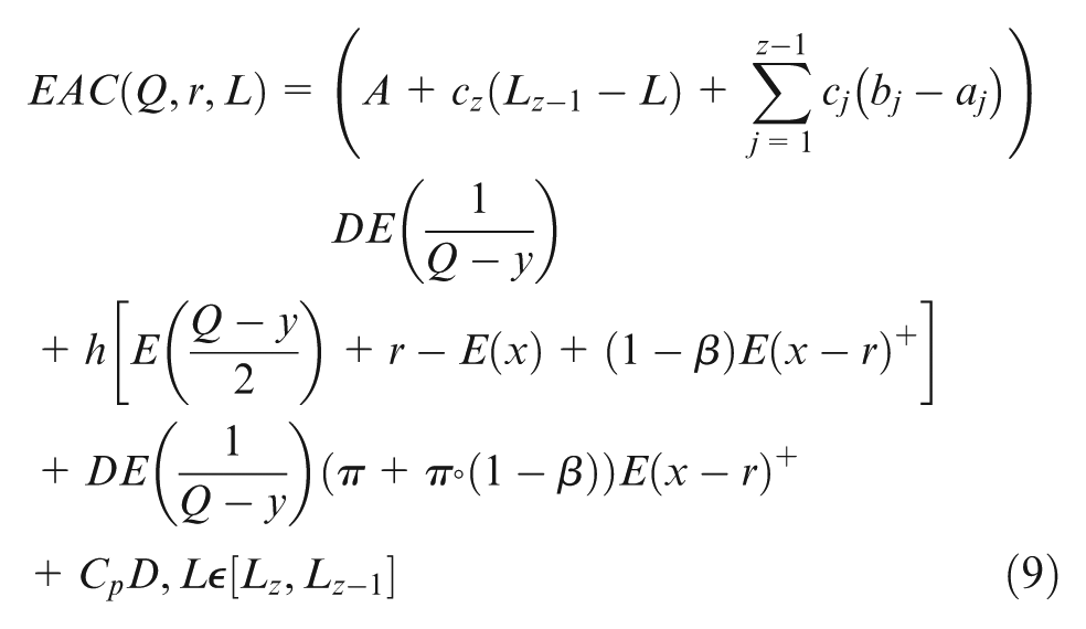
The underlying assumption in the above model (9) is that ordering cost, A, is a fixed constant and not subject to control. In this study, we consider that the ordering cost can be reduced through capital investment and it can be treated as a decision variable. Therefore, we seek to minimize the sum of capital investment cost of reducing ordering cost A and the inventory-related costs by optimizing over Q, A, r, and L constrained
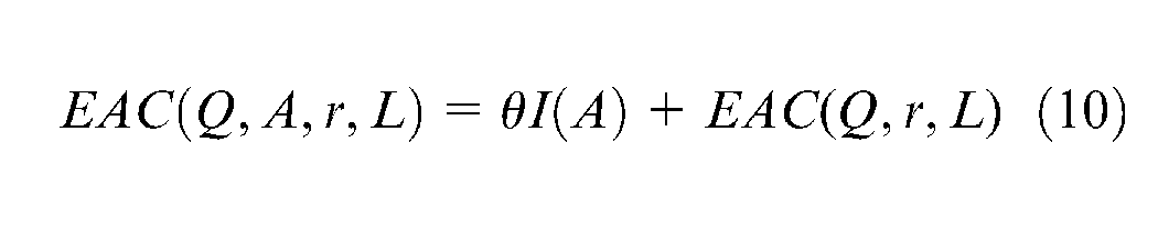
Over
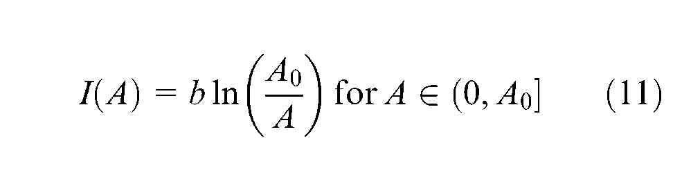
where
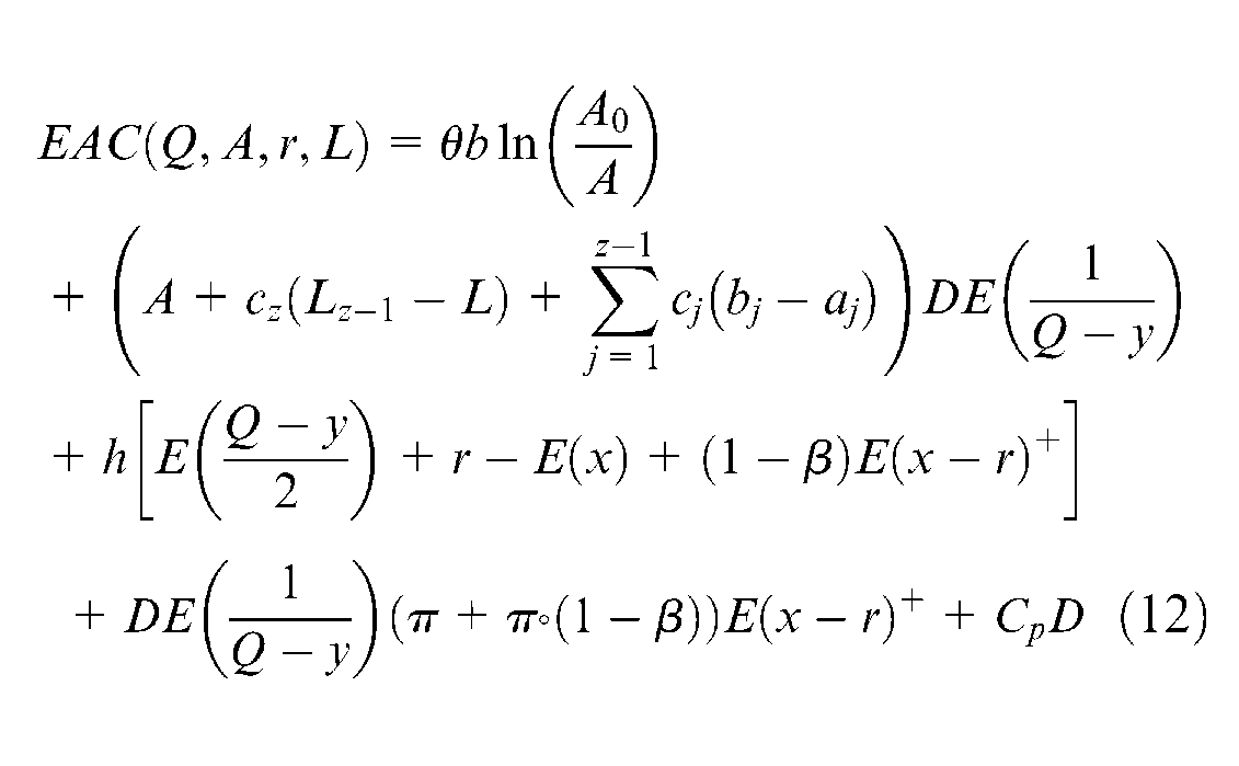
where
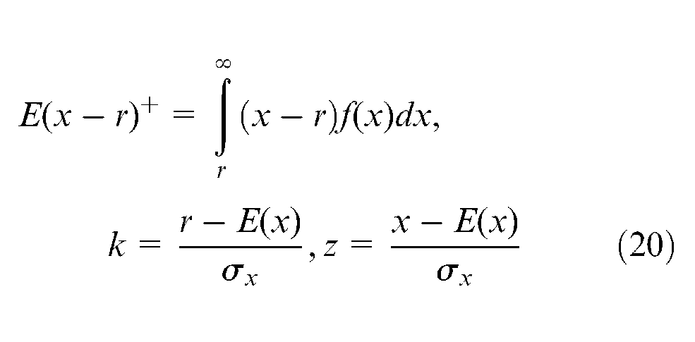
As we know, the following expected value is calculated 51
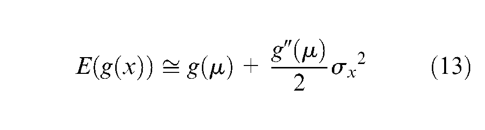
The above approximation for calculating expected value of a random quantity is accurate when standard deviation is small. Considering this assumption, the expected value of
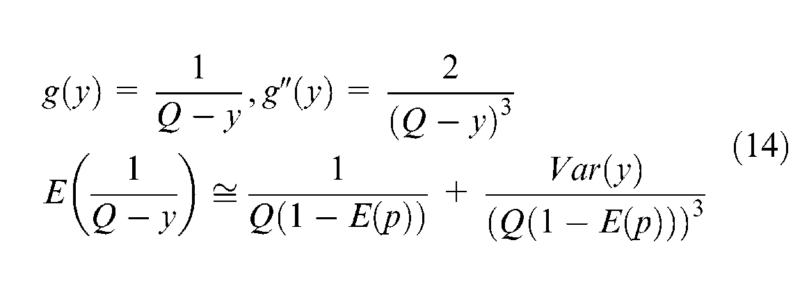
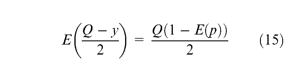
Besides, the expected value of
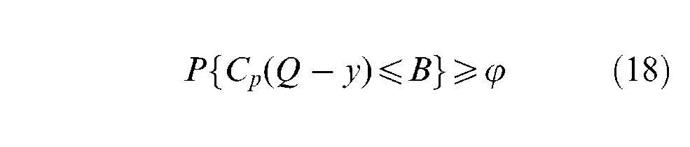
In this article, we consider a storage space restriction, which is dependent on the maximum inventory size. The restriction ensures that even if an item reaches to its maximum inventory position, the maximum available space is still enough for it. Therefore, the random storage space constraint for a partial backlogging policy is as follows
The above constraint forces the probability that total used space is within maximum permissible storage space to be no smaller than
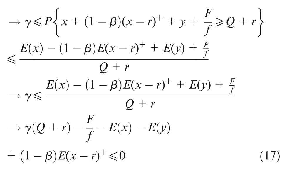
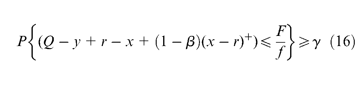
In this study, a restriction on the maximum available budget for purchasing is considered. In some cases, the available budget for purchasing is limited, and system managers would like to control it by considering this restriction on the inventory system. In this article, we assume that the purchasing costs are paid when an order arrives. With this assumption, we establish a limitation on the maximum available budget for purchasing. Thus, a form of the budget constraint is as follows

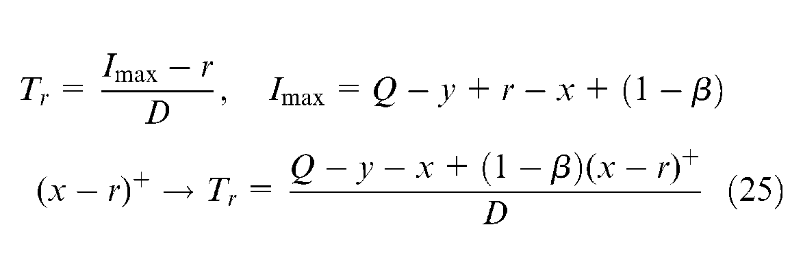
When the lead time demand
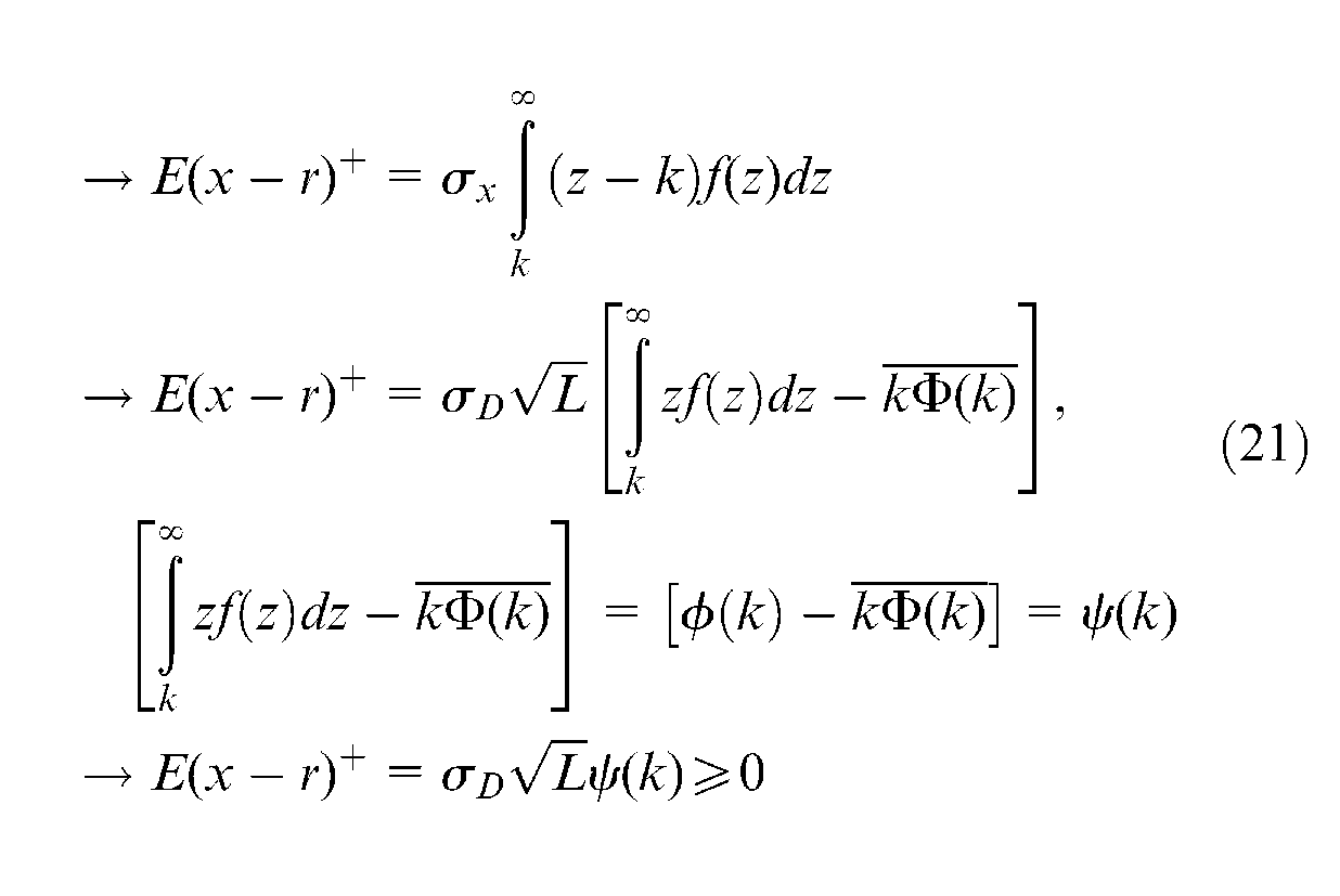
where
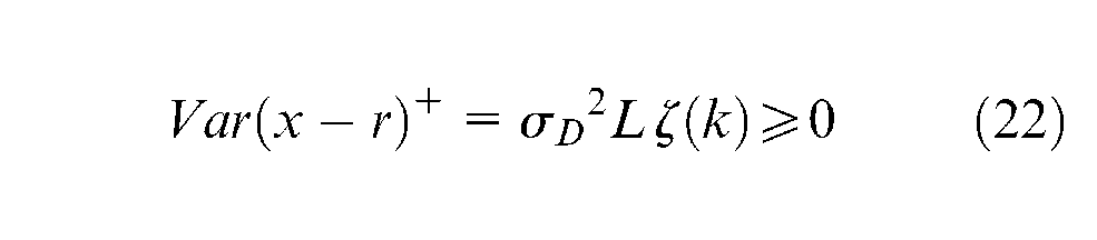
Also, variance of shortages is calculated as follows (see Appendix 3)
Therefore, considering
Subject to

where
Inspection model with reworking imperfect units
In this section, we consider the assumption of Rosenblatt and Lee 53 that imperfect items can be reworked instantaneously at a cost. Thus, the mathematical model can be expressed as follows

Subject to
Inventory inspection models with inflation
Inspection model without reworking imperfect units
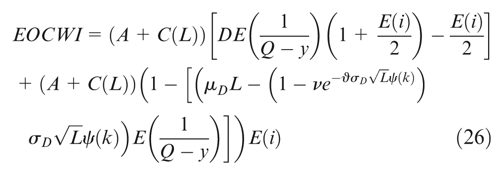
In this study, the average annual cost method with a stochastic inflationary condition is considered. In this article, we consider that the ordering cost will be paid at the time of the replenishment. Hence,
Expected ordering cost with inflation (EOCWI) is as follows (refer to Appendix 4)
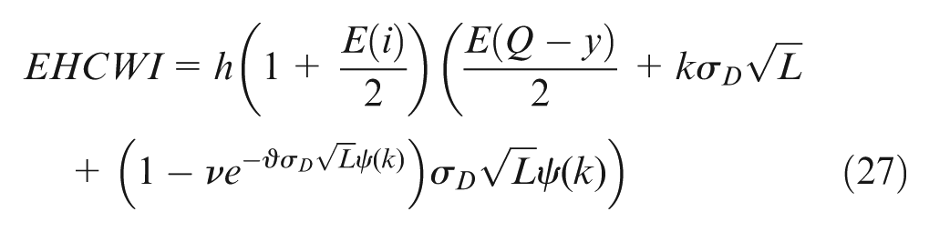
Total holding costs per year in the average annual cost method is dependent on the average inventory level. Therefore, expected holding cost per year with inflation (EHCWI) can be obtained as follows (refer to Appendix 5)
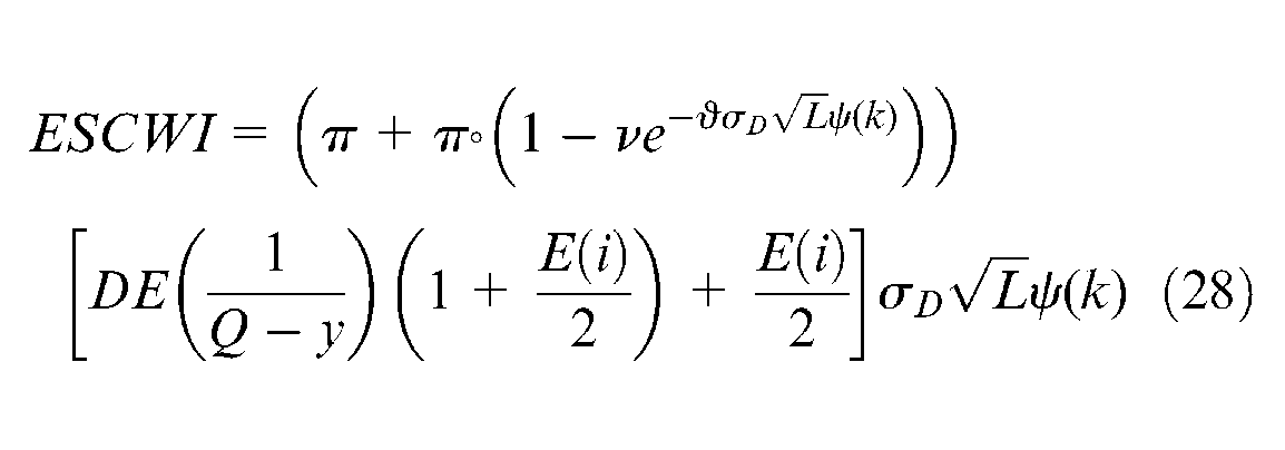
In this study, we assume that shortage cost is calculated at the end of cycle. Thus, expected shortage cost per year with inflation (ESCWI) can be obtained (see Appendix 6 for details)
In addition, we consider that the purchasing costs are paid at the beginning of the cycle. Hence, total expected purchasing cost with inflation (EPCWI) is as follows (refer to Appendix 7)
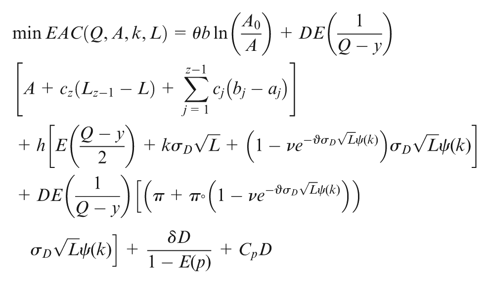
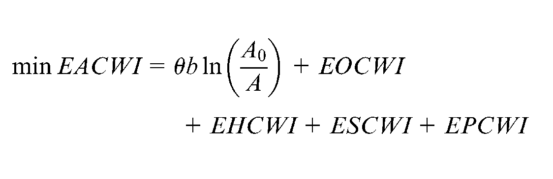
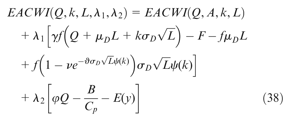
Therefore, the expected annual cost with inflation (EACWI) is the sum of equations (26)–(29). Thus, the multiobjective constrained model can be expressed as follows
Subject to

Note that if we do not have inflation rate (i = 0.00), then the above model (30) is converted to model (23).
Inspection model with reworking imperfect units
In this section, the inventory model’s total EOCWI is calculated as
The EHCWI can be expressed as follows
The ESCWI is
The total EPCWI can be calculated as follows
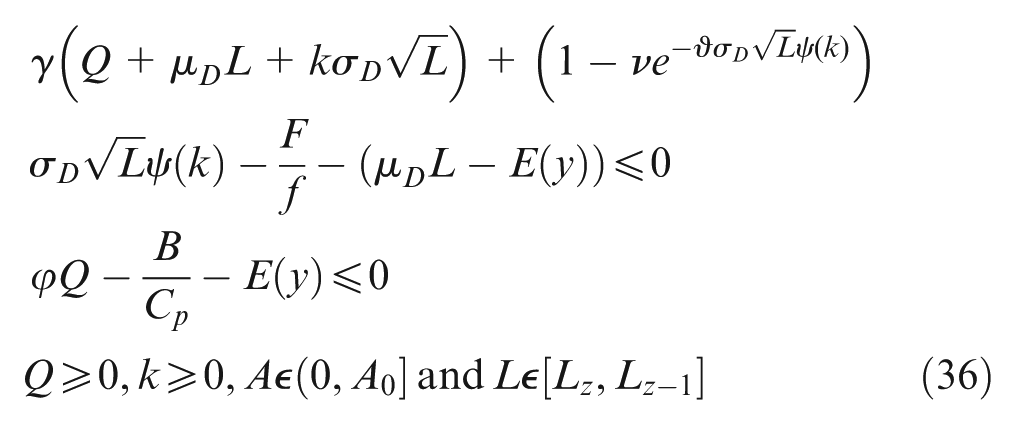
Therefore, our model is reduced to

Subject to
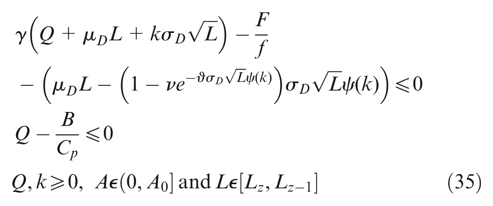
Note that if we do not have inflation rate (i = 0.00), then the above model (35) is converted to model (24).
Solution method
In this study, a heuristic method is utilized in order to solve multiobjective models. First, EAC function subjects to budget and storage space constraints is minimized as follows
Step 1.
Subject to
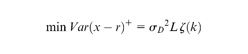
Second, variance of shortages is minimized in a distance of optimum point of first step as follows
Step 2.

Subject to
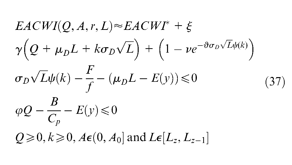
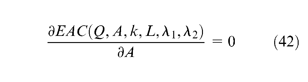
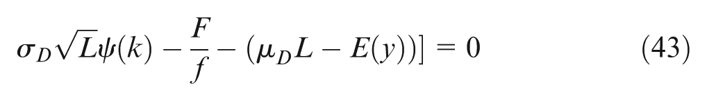
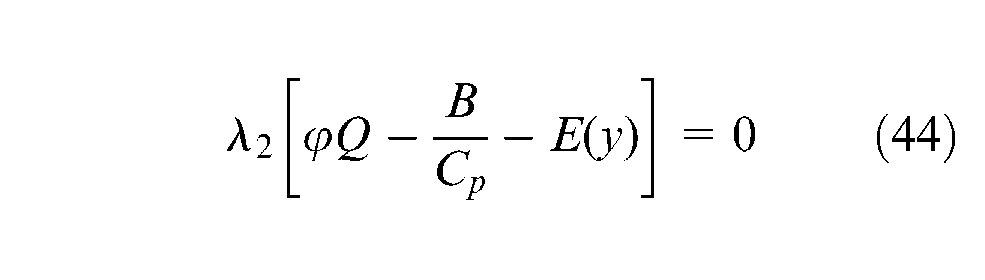
For Step 1, models (30) and (35) can be solved using Lagrange multiplier method with the same solution procedure. For instance, the Lagrangian function of the EAC function of model (30) is as follows
Notice that for any given
Hence, for fixed
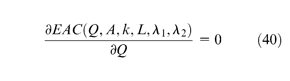
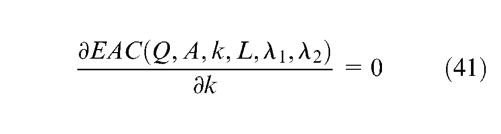
Since partial derivatives for these models are very complicated functions; hence, through the extensive testing, we assess the minimum values for the EAC for all models numerically.
Consequently, we can establish the following algorithm to find the optimal (
Step 1. For each
Step 1.1. Input the values of
Step 1.2. Compute
In this article, we consider
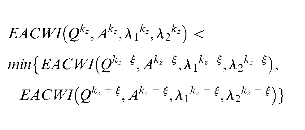
Step 2. Find
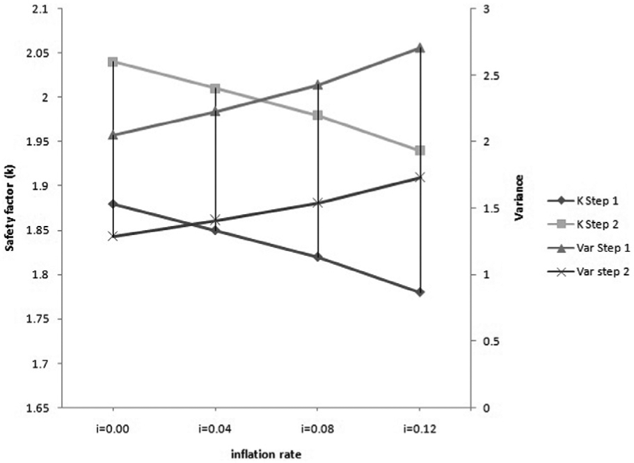
In the second optimization level, our goal is to minimize variance of shortages, which is dependent on safety factor and lead time variables. In this case, variance of shortages can be minimized by increasing safety factor or decreasing lead time in a distance (
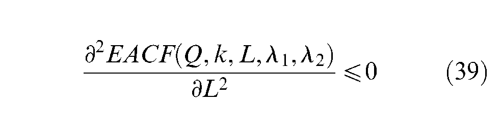
It is obvious that model (35) can be solved with the same solution procedure. Finally, compare the costs obtained for models (30) and (35) and choose the scenario with minimum cost. Moreover, to ensure the convexity of the constrained model of first step, the optimal values of
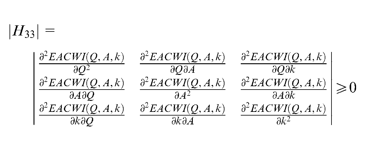
For a given value of L, we obtain the Hessian matrix H for objective function as follows
The first, second, and third principal minor of H must be positive for the optimal values
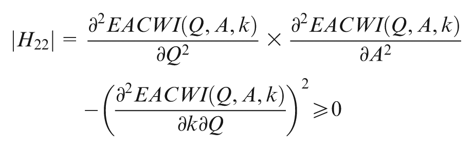
And
Also, for a given value of
Also, for a fixed
Numerical example
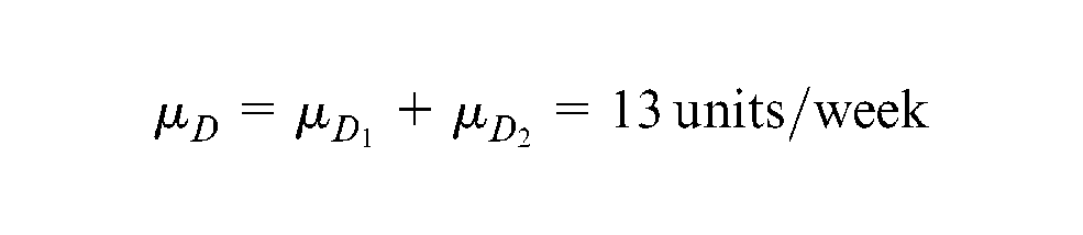
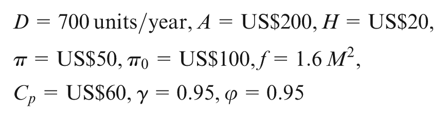
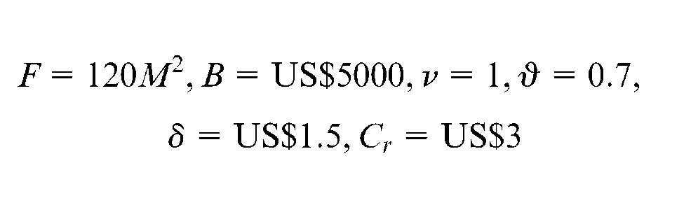
In this section, we solve some examples using the procedure outlined in the previous section. The purpose is to illustrate the solution procedure, conduct a sensitivity analysis for important model parameters and highlight important features of the developed models. The inventory system parameters are as follows
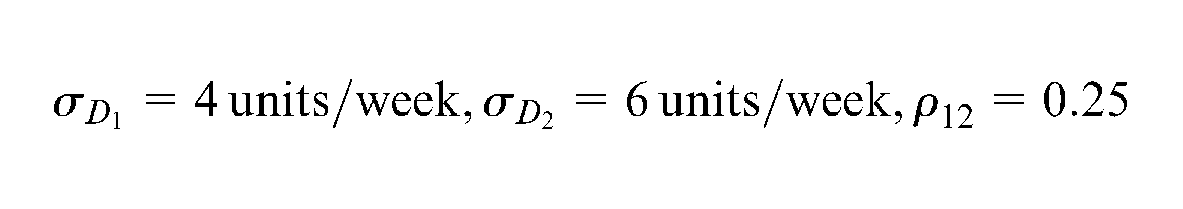
Hence, mean and standard deviation of demand are obtained as follows
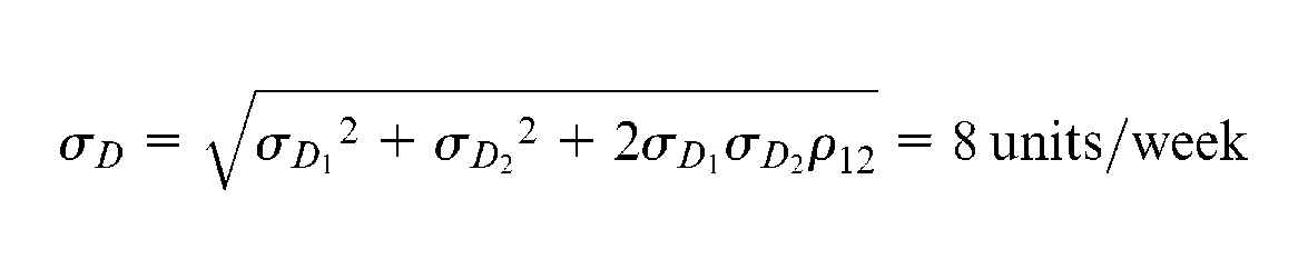
And
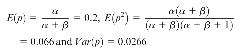
Defective rate
Therefore, we have
Besides, for the setup cost reduction, we take
Lead time data.
Results of first step of solution procedure for unconstrained model without reworking imperfect items (
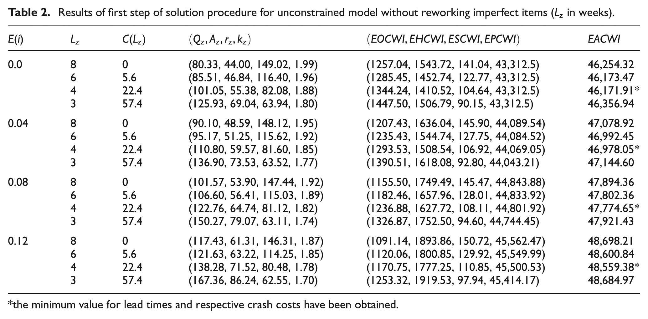
the minimum value for lead times and respective crash costs have been obtained.
Results of first step of solution procedure for unconstrained model with reworking imperfect items (
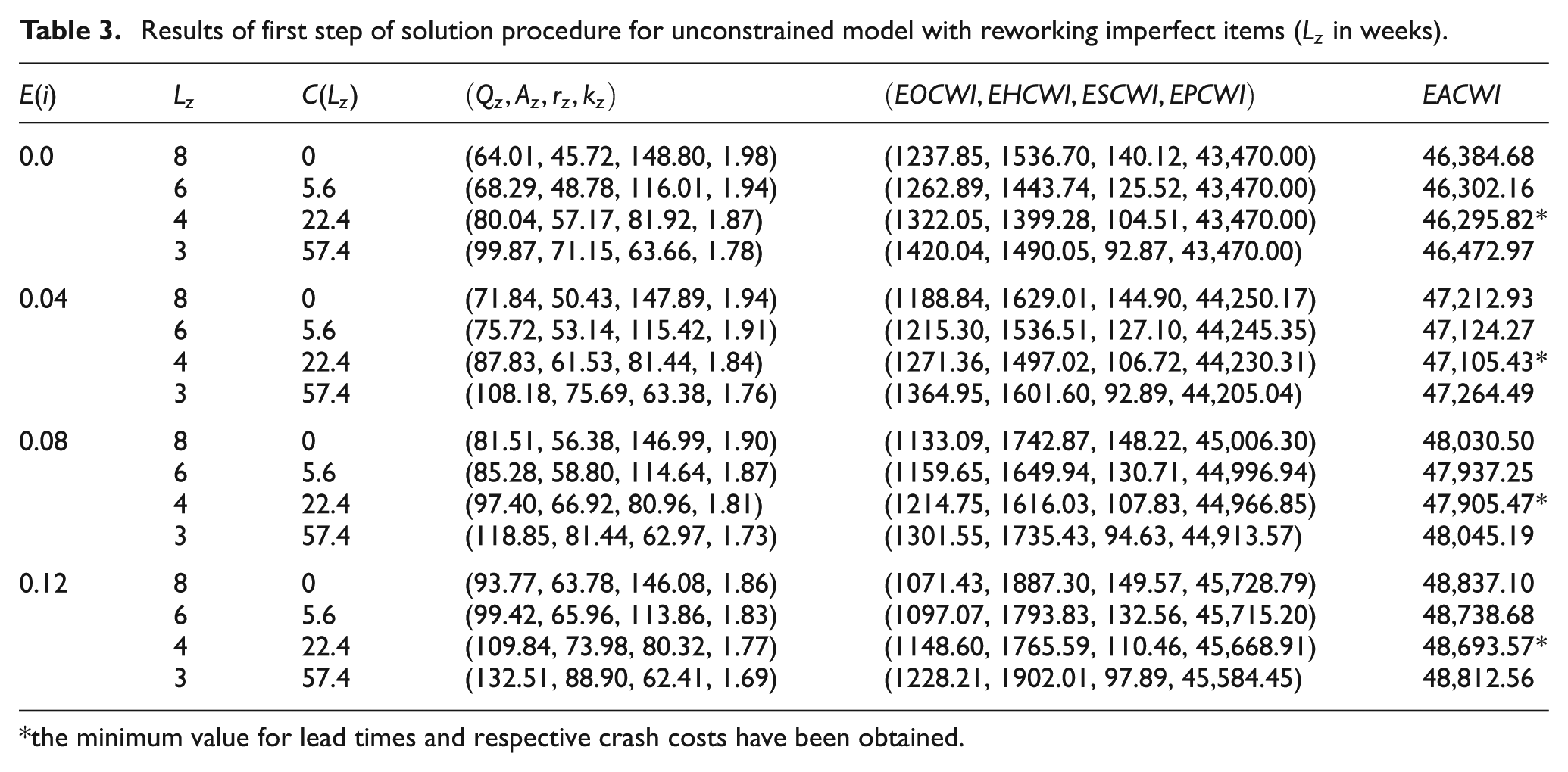
the minimum value for lead times and respective crash costs have been obtained.
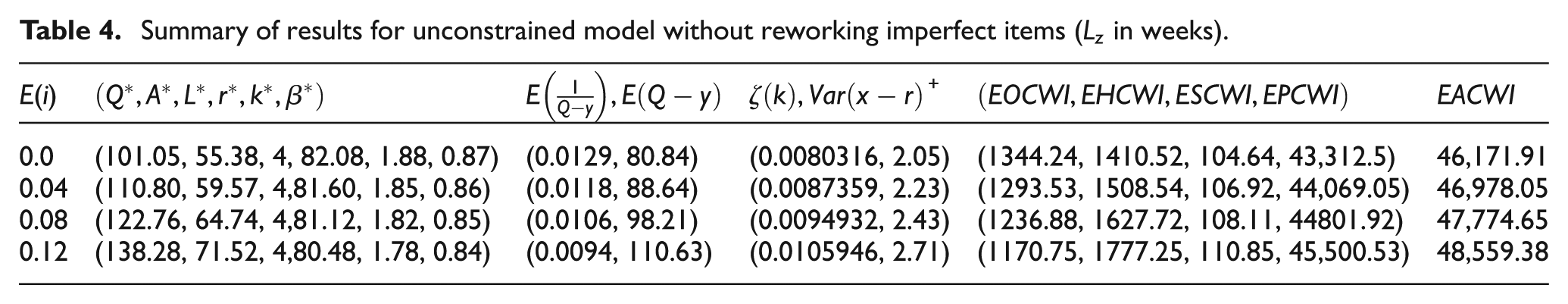
Summary of results for unconstrained model without reworking imperfect items (
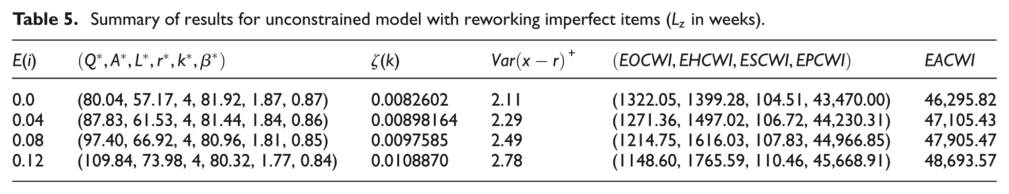
Summary of results for unconstrained model with reworking imperfect items (
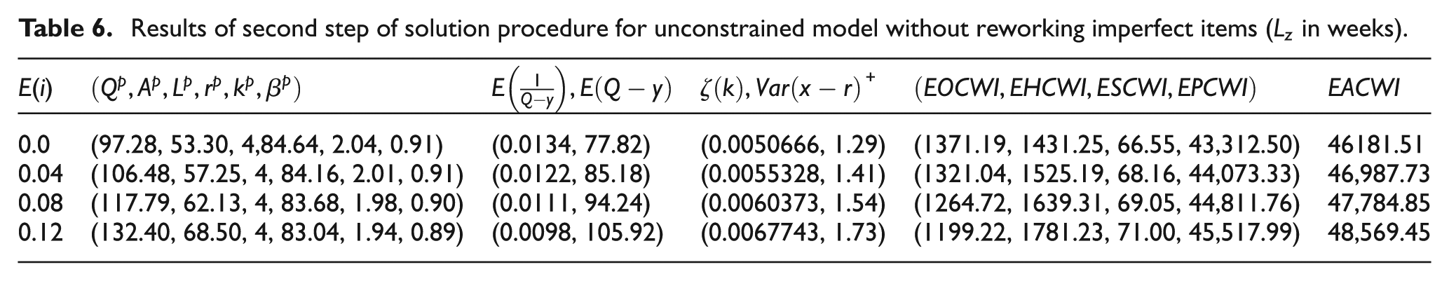
Results of second step of solution procedure for unconstrained model without reworking imperfect items (
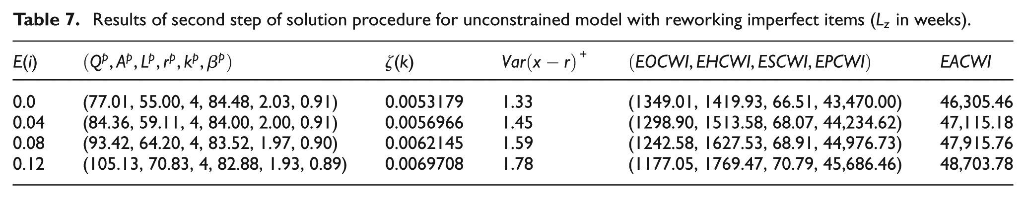
Results of second step of solution procedure for unconstrained model with reworking imperfect items (
Optimal EACWI values in terms of different safety factor (k).
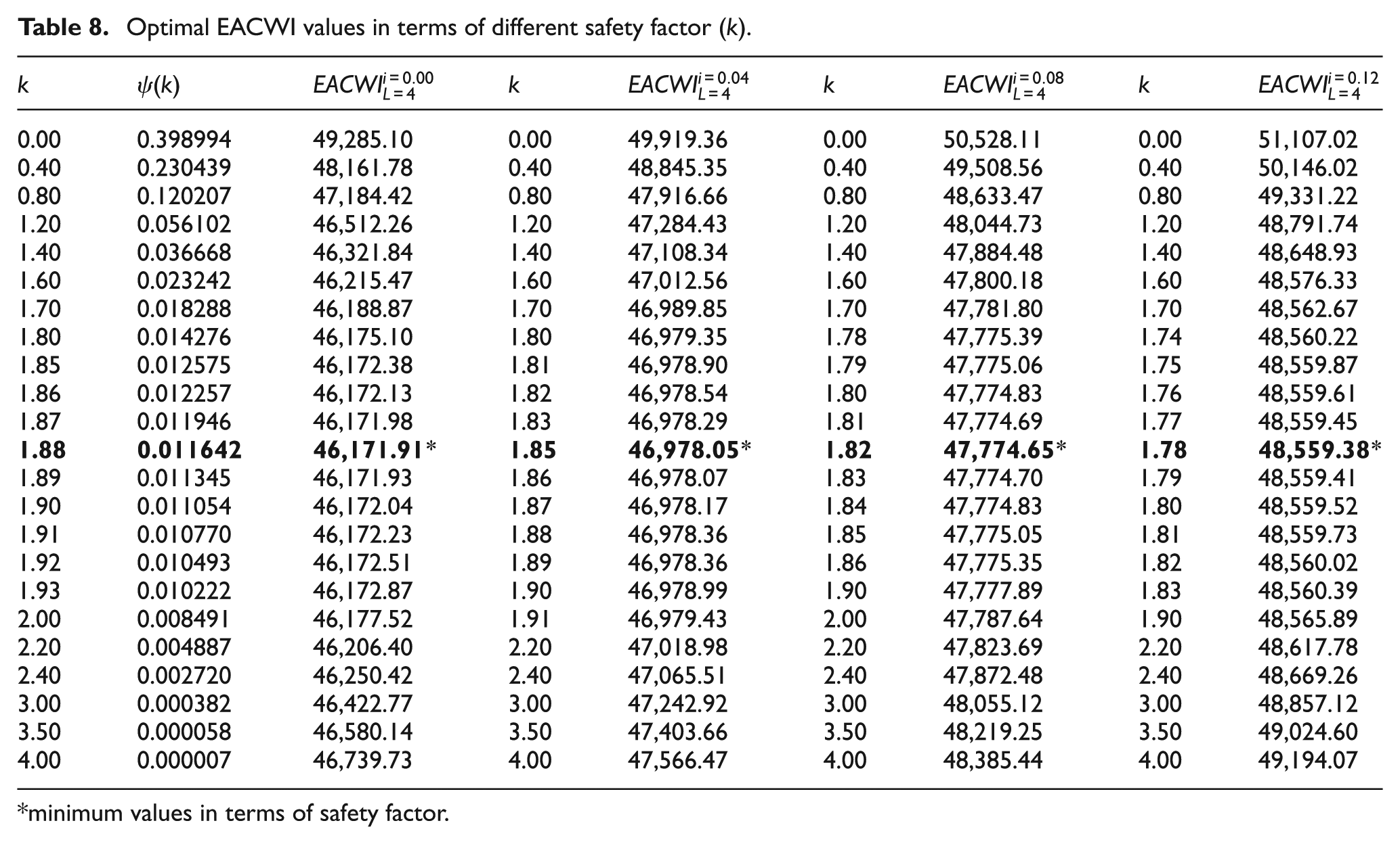
minimum values in terms of safety factor.
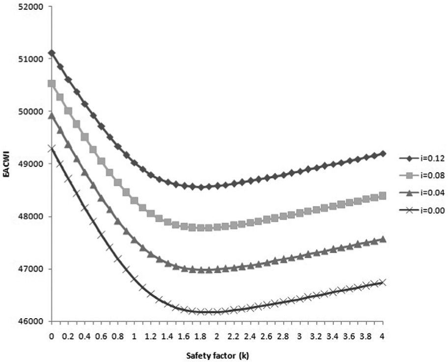
Convexity of model in terms of various safety factor (k).
Optimal order quantity in terms of various lead time and inflation rates.
Multiobjective model performance for variance of shortages.
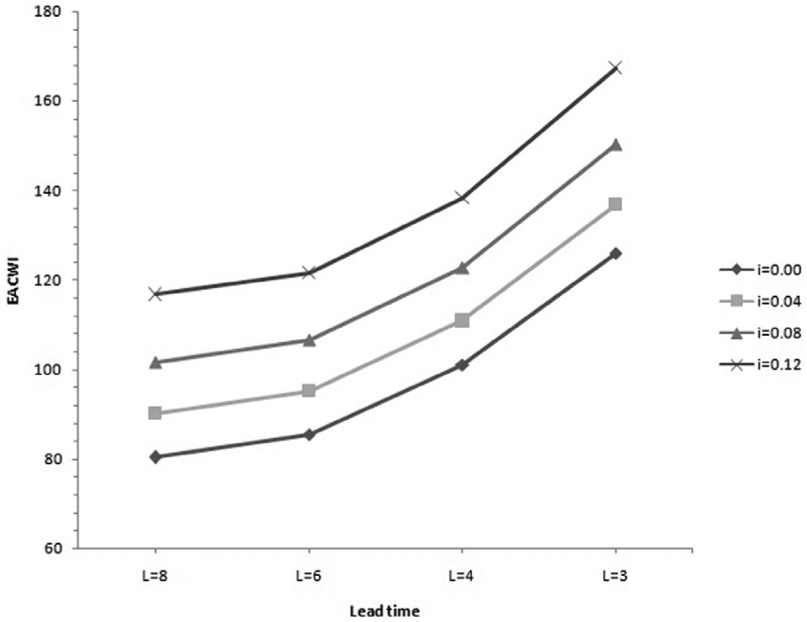
The optimal values of the constrained inventory inspection models in the first step are tabulated in Tables 9 and 10 for
Results of first step of solution procedure for the constrained model without reworking imperfect items (
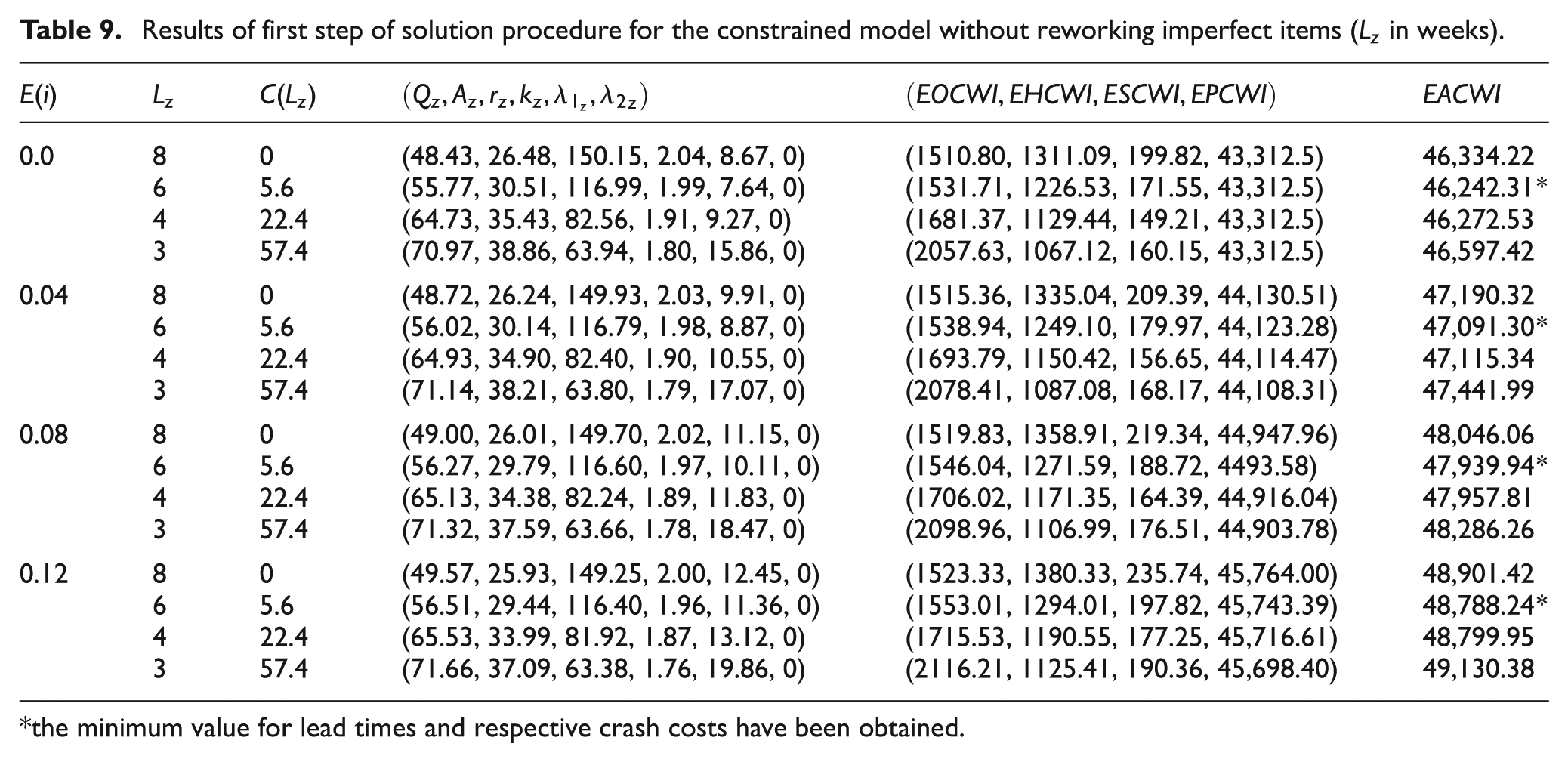
the minimum value for lead times and respective crash costs have been obtained.
Results of first step of solution procedure for the constrained model with reworking imperfect items (
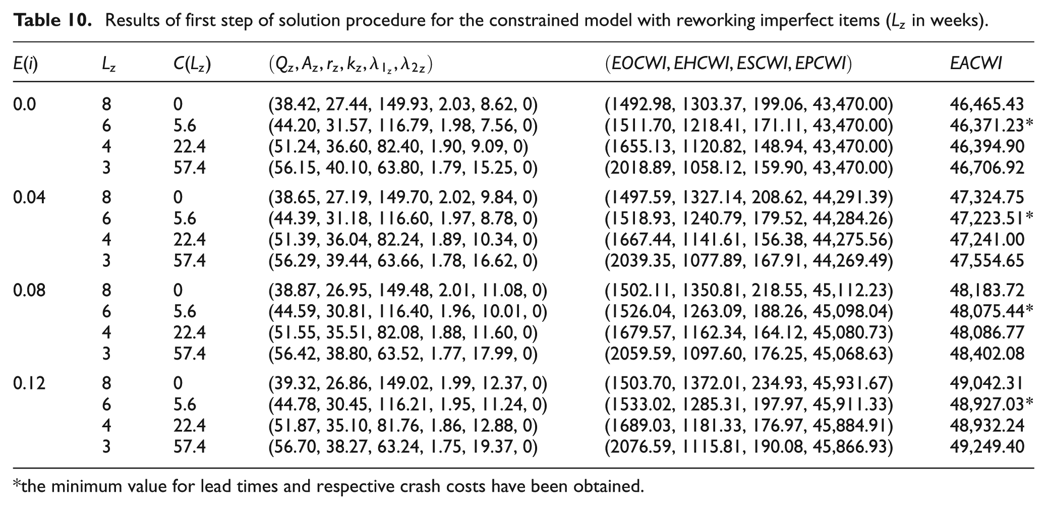
the minimum value for lead times and respective crash costs have been obtained.
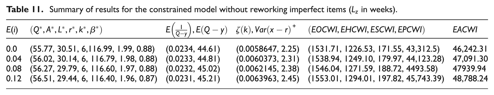
Summary of results for the constrained model without reworking imperfect items (
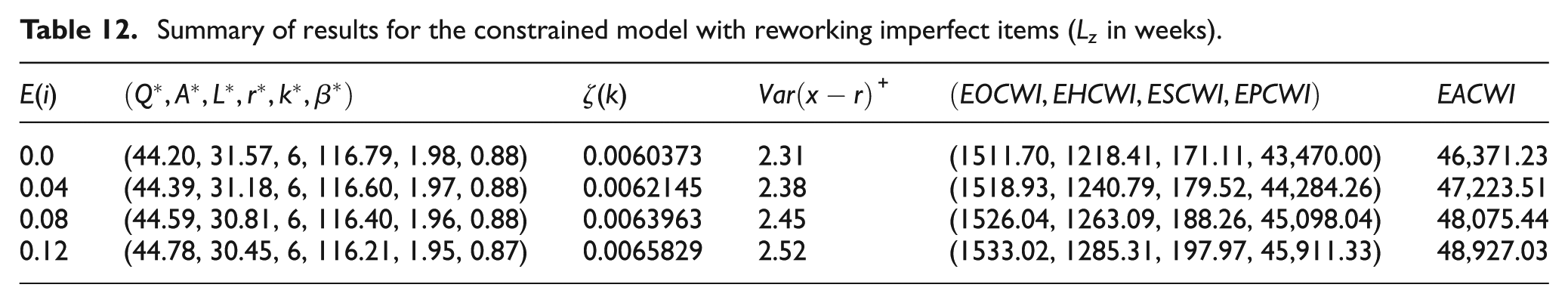
Summary of results for the constrained model with reworking imperfect items (
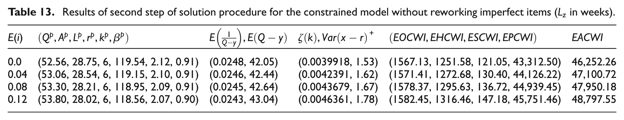
Results of second step of solution procedure for the constrained model without reworking imperfect items (
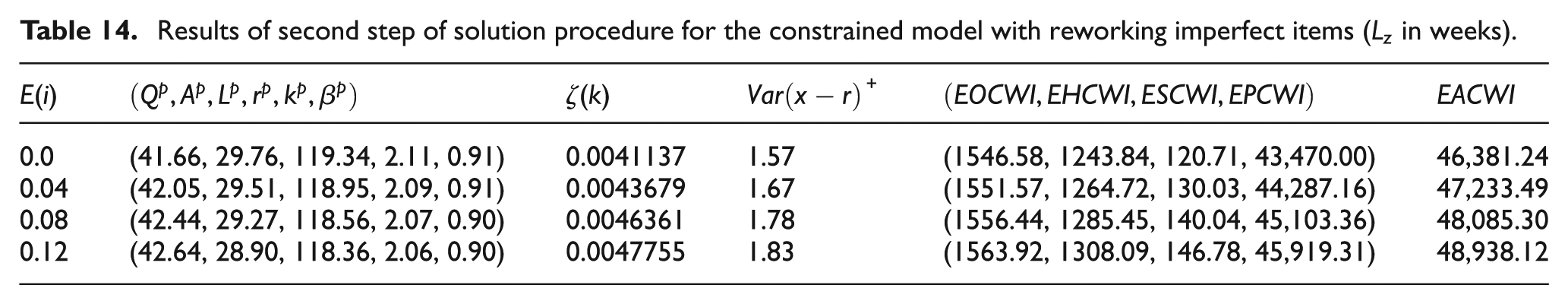
Results of second step of solution procedure for the constrained model with reworking imperfect items (
In the discussed inventory system’s data, it is considered that the defective rate follows a beta-distribution function with a small standard deviation. Moreover, in order to show that this assumption is met for the data used in the respective system, a column is added in Tables 4, 6, 11, and 13 for unconstrained and constrained inventory models with discarding defective units, and the values of
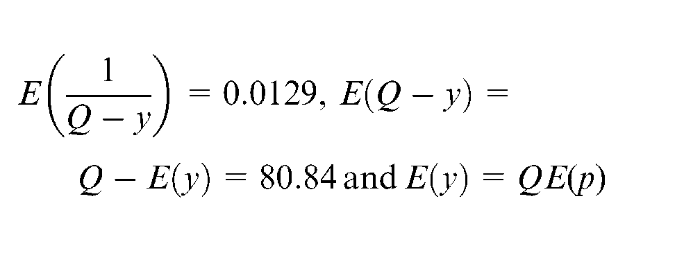
We know that
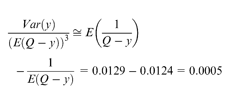
The above calculations show that the effect of variance of defective units is low and the obtained expected value is very close to the situation of fixed defective rate. Also, we know that the expected number of cycle equals
The change in the values of system parameters can take place due to uncertainties and dynamic market conditions in any DM situation. In order to examine the implications of these changes in the value of parameters, the sensitivity analysis will be of great help in a DM process. By using the previous numerical example, the sensitivity analysis of various parameters has been carried out in this article. Results of sensitivity analysis are shown in Table 15. Finally, the main conclusions, one can draw from the sensitivity analysis, are as follows:
Effect of changes in various parameters.
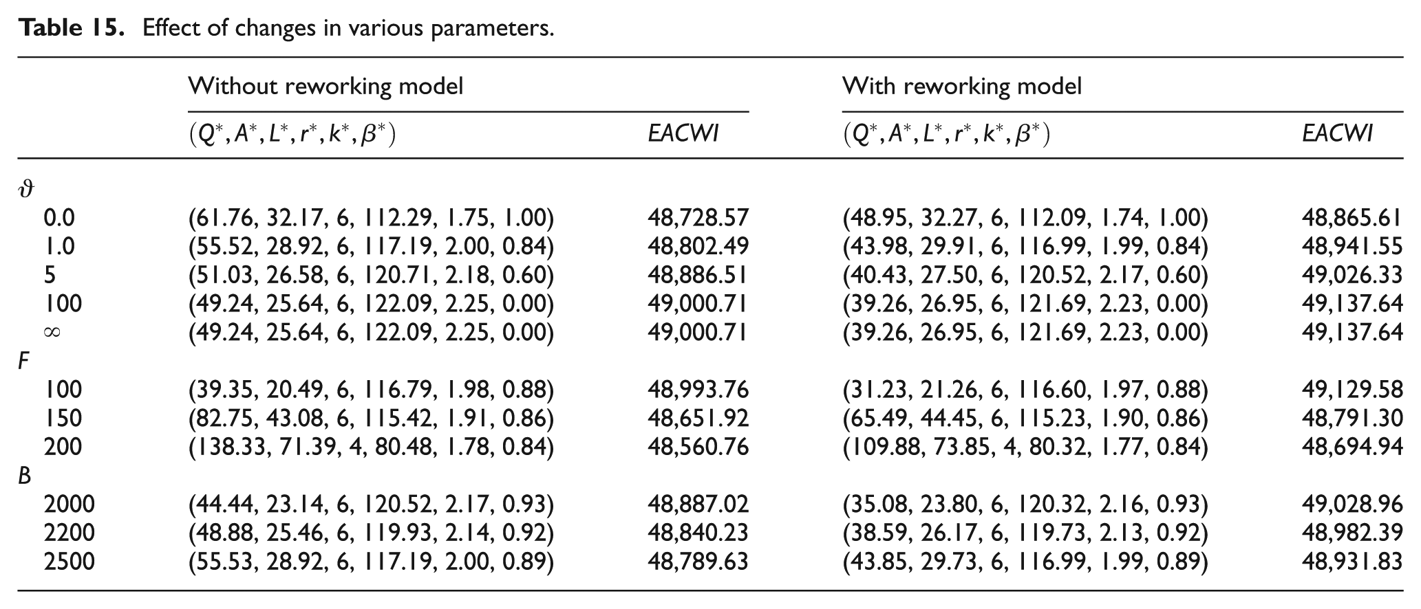
Keeping all the parameters fixed, if the value of
With an augment in the maximum available space (F) and keeping the remaining parameters unchanged, the optimal order quantity (
With an increase in maximum inventory investment (B) and keeping the remaining parameters fixed, the optimal order quantity (
Conclusion
In this article, we explored multiobjective multiconstraint stochastic inventory inspection models with and without reworking of imperfect items discovered during inspection. The imperfect items in a lot are assumed to be random variable. The objectives are to minimize EAC and variance of shortages. Lead time and ordering cost are assumed to be controllable. Backorder rate is dependent on the length of lead time through the amount of shortages. Hence, with mixture of backorder and lost sales, this study assumes the order quantity, reorder point, lead time, ordering cost, and backorder rate as decision variables. A random storage space constraint is considered since the inventory level is random when an order arrives. So, in this case, a chance-constrained programming technique is used to make it crisp. A budget constraint is also added to the model. The piece-wise linear crashing cost function that is widely used in project management is considered in this article. This article assumes that the lead time demand follows a normal distribution. A numerical example is also given to illustrate model and its solution procedure. The proposed model can be extended in several directions. For instance, we may consider sampling inspection in the models or optimizing model for periodic review policy instead of continuous review policy.
Footnotes
Appendix 1
Appendix 2
It is considered that defective items in an order lot to be a random variable (y), which has a beta-binomial distribution with parameters (
In this case, we have
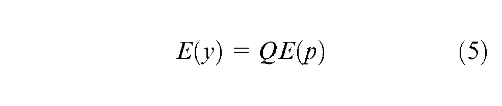
Hence, unconditioning on p, the expected value of
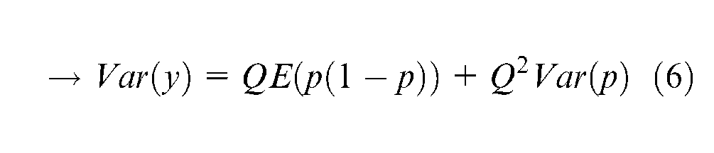
The variance of
Appendix 3
Variance of shortages is calculated as follows
And
Hence, variance of shortages is as follows
Appendix 4
The total ordering cost per year paid at the time of order placing is computed as follows ((
So, the total ordering cost paid at the time of order placing can be expressed by
Hence, equation (62) can be written as
By considering
Therefore, considering
Appendix 5
Total holding cost per year is a random variable and can be computed as follows
Hence, considering
Therefore, considering
Appendix 6
The average shortage cost per year per unit with inflation is calculated by (
By multiplying the average stock out cost in the number of cycle (n), the total shortage cost per year is obtained by (
Hence, by considering
Therefore, considering
Appendix 7
The average purchasing cost per unit is obtained as follows
Hence, considering (I, X, Y) as independent, the expected purchasing cost is obtained by
Also, the expected inspecting cost is as follows
Therefore, the expected total purchasing cost with inflation (EPCWI) is
Acknowledgements
The authors gratefully acknowledge the constructive comments made by the anonymous referees on an earlier version of this article.
Conflict of interest
The authors declare that there is no conflict of interest.
Funding
This research received no specific grant from any funding agency in the public, commercial, or not-for-profit sectors.