Sage Journals: Discover world-class research

Abstract

In this article, an integrated production–distribution model is presented for a manufacturer and retailer supply chain under inflationary conditions, permissible delay in payments, deterioration, imperfect production process and inspection errors. We assume that the first-stage inspection of the manufacturer is not perfect and makes inspection errors of Type 1 and Type 2. The second-stage inspection of the manufacturer is at the end of production period without inspection errors. Also, the demand is linear function of time. Once the retailer receives the lot, a 100% screening process of the lot is conducted without inspection errors, and the screening process and demand proceed simultaneously. The main objective is to determine the optimal inspection time and the optimal number of cycle such that the present value of the total cost is minimized. Finally, a numerical example and sensitivity analyses are provided to illustrate the proposed model using a proper algorithm.

Keywords

Supply chain inventory deterioration imperfect items delay in payments inflation inspection errors

Introduction

Recently, firms have focused on supply chain management and have been attempting to achieve greater collaborative advantages with their supply chain partners. Since firms realize that inventory across the supply chain can be more efficiently managed through greater cooperation and better coordination, integrated inventory management has recently received a great deal of attention. In practice, suppliers frequently offer retailers many incentives such as a permissible delay in payments to attract new customers and increase sales. The effect of delays in payments in the optimal pricing and inventory control for non-instantaneously deteriorating items has been considered by some researchers. In addition, the effect of inflation and time value of money cannot be ignored in global economics. Furthermore, in real-life situations, there is inventory loss by deterioration and the inventory value is dependent on the product value at the time of evaluation. Deterioration means decay, evaporation, obsolescence, loss of quality or marginal value of commodity. Obviously, deterioration decreases the usefulness of the good from its original condition. The longer the goods are kept in inventory, the higher the deteriorating cost. However, imperfect items are produced due to non-ideal production processes. Therefore, the lot sizes produced/received may contain certain percentage of defective items.

As far as we know, this is the first model in the supply chain models that considers deterioration, defectiveness, inspection errors, permissible delay in payments and inflation in which production is delivered in n equal size shipments after producing all products. An appropriate algorithm is presented to derive the optimal inspection time and the optimal number of cycle such that the present value of the total cost is minimized. A numerical example and sensitivity analyses are provided to illustrate the proposed model.

Following this, notations and assumptions are presented in section “Notations” and “Assumptions.” In section “Model description,” we organize the mathematical models. Then, section “Optimal solution procedure” presented an algorithm to find the optimal inventory variables. The numerical example is provided in section “Numerical example.” Next, a sensitivity analysis is presented in section “Sensitivity analysis.” Finally, discussion of the results as well as directions for future study is presented in section “Conclusion.”

Literature review

In the past, most studies on the supply chain, the vendor and the buyer were considered to be independent from each other with different objectives and self-interest. Because of raising the costs, globalization trend, short life time of products and increasing the importance of quick response to customer’s needs, more attentions has been focused on the integration of the whole supply chain system. Goyal¹ considered an integrated supply chain with one supplier and one buyer for the first time. Lo et al.² investigated an integrated supply chain with one manufacturer and one retailer for deteriorating items with assumptions of imperfect items, inflation and partial backordering. Yan et al.³ developed an integrated production–distribution model in a two-echelon supply chain considering deteriorating item and multiple deliveries. Moussawi-Haidar et al.⁴ considered a three-level supply chain, consisting of a capital-constrained supplier, a retailer and a financial intermediary (bank), coordinating their decisions to minimize the total supply chain costs considering delay in payments.

In the previous inventory models, it was assumed that the payment must be made to the manufacturer for items immediately after receiving the supplies. But in real situation, the manufacturer allows a certain delay period to entice the retailer to buy more and does not pay the retailer any interest on the amount during this period. However, during the trade credit period, the retailer earns interest on the payment received for the goods sold and thus accumulates revenue. Therefore, the effects of manufacturer credit policies have received the attention of many researchers. Goyal⁵ investigated a single-item inventory model considering a permissible delay in payments. Ouyang et al.⁶ considered the inventory model for non-instantaneous deteriorating items with permissible delay in payments. Hu and Liu⁷ developed an optimal replenishment policy for the economic production quantity (EPQ) model under permissible delay and allowable shortages. Maihami and Nakhai Kamal Abadi⁸ developed an inventory model with assumption of non-instantaneous deterioration items in which delay in payments and partial backlogging is considered. Jana et al.⁹ presented an integrated production-inventory model for a supplier, manufacturer and retailer supply chain under conditionally permissible delay in payments in the uncertain environments. Chern et al.¹⁰ derived a vendor–buyer supply chain model with permissible delay in payments under non-cooperative Nash equilibrium.

In the past, most studies on supply chain management and the effect of inflation were not considered. This was due to the belief that most of the decision makers believe that inflation does not have considerable influence on the inventory policy and thus do not consider the effect of inflation on the inventory system. But in real situations, the resource of a firm is highly correlated to the return of the investment. So, the concept of the inflation should be considered especially for long-term investment and forecasting. First, Buzacott¹¹ considered an economic order quantity (EOQ) model with inflation for the first time. Sarker et al.¹² investigated a model to determine an optimal ordering policy for deteriorating items under inflation, permissible delay of payment and allowable shortage. Sarkar and Moon¹³ improved a production-inventory model considering stochastic demand and inflation. Guria et al.¹⁴ proposed an inventory model with inflation and selling price dependent demand under finite and random planning horizon allowing trade credit against immediate part payment. Ghoreishi et al.¹⁵ developed an inventory model for non-instantaneous deteriorating items considering inflation and customer returns. Ghoreishi et al.¹⁶ studied the effects of delay in payments, customer returns and inflation for an EPQ model for non-instantaneous deteriorating items and price- and time-dependent demand.

Currently, deteriorating inventory is becoming more important. Because in real life, most of the products, such as medicine, fruits and vegetables, are deteriorating items. Deterioration plays an important role in inventory management and also in all other elements of the production process where items are stocked or forced to wait due to uncertain demand, technical matters or disruptions of the production process. Ghare and Schrader¹⁷ proposed a model with exponential decay initially. Skouri et al.¹⁸ discussed a model with general ramp-type demand rate, time-dependent (Weibull) deterioration rate and partial backlogging of unsatisfied demand under different replenishment policies. Das et al.¹⁹ developed a production-inventory model for a deteriorating item with stock-dependent demand under two storage facilities over a random planning horizon, which is assumed to follow exponential distribution with known parameter. Wee and Widyadana²⁰ developed a production model for deteriorating items with stochastic preventive maintenance time and rework considering the first in first out (FIFO) rule with uniform and exponential distribution preventive maintenance time. Sicilia et al.²¹ studied a deterministic inventory system for items with a constant deterioration rate, time-dependent demand and shortages.

In the traditional inventory models, it was assumed that 100% of the items are perfect, whereas the produced items may contain defective items because of deficient maintenance, weak production control and so on. Therefore, the screening process is done to distinguish the imperfect items. Also, there could be some imperfect errors in the inspection process. Recently, the imperfect production process has been investigated by many researchers. Rosenblatt and Lee²² proposed an EPQ model considering imperfect items, where the elapsed time from in-control state to out-control state is assumed to be a random variable. Goyal et al.²³ developed a simple approach for determining an optimal integrated vendor–buyer policy for imperfect items. Khan et al.²⁴ investigated an EPQ model with imperfect items and imperfect screening process. Sana²⁵ discussed an integrated production-inventory model for supplier, manufacturer and retailer supply chain, considering perfect and imperfect quality items. Yoo et al.^26,27 investigated imperfect production and inspection errors, investment in production and inspection reliability with one-time and continuous improvement and defective disposal with customers’ return. Lee and Kim²⁸ extended an integrated production–distribution model to determine an optimal policy with both deteriorating and defective items. Table 1 gives the summary of the literature review.

Table 1.

Summary of literature review.

Article	The level of supply chain			Deterioration rate			Imperfect items	Shortage	Demand rate					Ordering policy			Other conditions
Article	Two-level	Three-level	More than members in each level	Constant	Non-instantaneous	Time-dependent	Imperfect items	Shortage	Constant	Time-dependent	Price-dependent	Time- and price-dependent	Stochastic	Lot-for-lot	Delayed equal-sized shipment	Non-delayed equal-sized shipment	Inflation	Delay in payment
Goyal (1976)¹	*
Lo et al. (2007)²	*					*	*	÷*	*								*
Yan et al. (2011)³																*
Moussawi-Haidar et al. (2014)⁴		*					*	*		*								*
Goyal (1985)⁵																		*
Ouyang et al. (2006)⁶	*										*					*		*
Hu and Liu (2010)⁷								*	*									*
Maihami and Nakhai Kamal Abadi (2012)⁸					*			*				*						*
Jana et al. (2013)⁹		*						*	*									*
Chern et al. (2014)¹⁰	*															*		*
Buzacott (1975)¹¹																	*
Sarker et al. (2000)¹²				*				*			*						*	*
Sarkar and Moon (2011)¹³							*						*				*
Guria et al. (2013)¹⁴								*			*						*
Ghoreishi et al. (2014)¹⁵					*							*					*
Ghoreishi et al. (2014)¹⁶					*							*					*	*
Ghare and Schrader (1963)¹⁷					*
Skouri et al. (2009)¹⁸						*		*					*
Das et al. (2012)¹⁹				*					*								*
Wee and Widyadana (2014)²⁰				*				*	*
Sicilia et al. (2014)²¹				*				*		*
Rosenblatt and Lee (1986)²²							*
Goyal et al. (2003)²³	*						*
Khan et al. (2011)²⁴	*						*			*						*
Sana (2011)²⁵		*					*
Yoo et al. (2009)²⁶							*		*
Yoo et al. (2012)²⁷							*		*
Lee and Kim (2014)²⁸	*						*		*							*
Taheri-Tolgari et al. (2012)²⁹							*		*								*
Geetha and Uthayakumar (2010)³⁰					*			*	*									*
This study	*				*		*			*						*	*	*

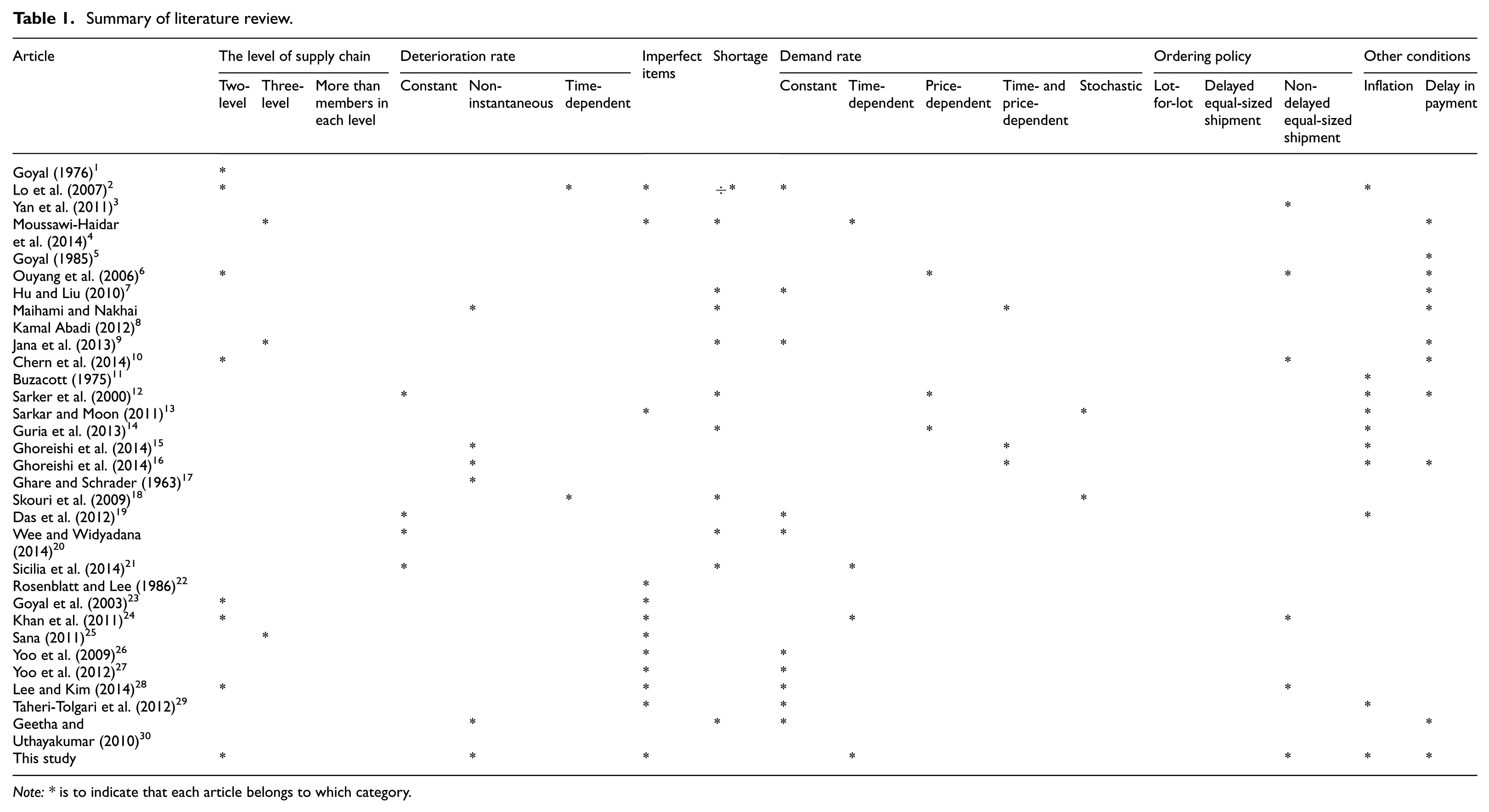
Note: * is to indicate that each article belongs to which category.

In dealing with these shortcomings above, we develop an inventory model for deteriorating items, with imperfect quality, inspection errors and permissible delay in payments in two-level supply chain under inflationary conditions. We assume that demand is time-dependent. Also, we investigated a supply chain with one manufacturer and one retailer, where the production process and inspection process are not perfect. The lot size of Q is produced and inspected at the production rate of p. The production items contain defective items of $α$ percent with a known probability density function (pdf) of $f (α)$ . The inspection errors occur at the first-stage inspection of the manufacturer with proportions of $β$ and $γ$ . According to Taheri-Tolgari et al.,²⁹“the proportions $β = pr$ (items screened as defective–non-defective items) and $γ = pr$ (items non-screened as defective–defective items) ( $0 < β, γ < 1$ ). We assume $β$ and $γ$ are independent of a defect proportion $α$ .” As a result, in the entire lot inspection process during $[0, t_{1}]$ , $(1 - α) β Q_{1 m}$ units among the perfect items of $(1 - α) Q_{1 m}$ are falsely screened out and treated as defective items and $(1 - α) (1 - β) Q_{1 m}$ treated as serviceable items. Also, $α γ Q_{1 m}$ units among the defective items of $α Q_{1 m}$ are falsely treated as serviceable items. So, $α (1 - γ) Q_{1 m}$ are successfully screened out. Therefore, the serviceable items of $α γ + (1 - α) (1 - β)) Q_{1 m}$ can satisfy the retailer demand and $α (1 - γ) + (1 - α) β) Q_{1 m}$ of lot $Q_{1 m}$ in each cycle are removed from the inventory level. Then, in the second-stage inspection of the manufacturer at time $t_{2}$ , it is assumed that there are no inspection errors and only $α$ percent of produced items during $[0, t_{1}]$ is removed from the inventory level and leaving $(1 - α)$ percent of them passed on to the retailer. As soon as the retailer received the order quantity, the 100% inspection process is done in which there are no inspection errors and $α γ q$ of order quantity are removed.

Methodology and model building

The following notations are used throughout the article.

Notations

A ordering cost for the retailer

$a, b > 0$ constant parameters of demand

c production cost per unit

$c_{1}$ purchasing cost per unit for the retailer

D demand rate

$ETC$ expected value of total cost of the whole supply chain

$ET C_{m}$ expected value of total cost of the manufacturer

$ET C_{r}$ expected value of total cost of the retailer

$h_{m}$ inventory holding cost per unit for the manufacturer

$h_{r}$ inventory holding cost per unit for the retailer

H length of planning horizon

$I_{e}$ interest earned per dollar per unit time

$I_{im} (t)$ inventory level i at time t for manufacturer in production period, $i = 1, 2$

$I_{ir} (t)$ inventory level i at time t for the retailer, $i = 1, 2, 3$

$I_{m}^{j} (t)$ inventory level i at time t for manufacturer in non-production period, $j = 1, \dots, n$

$I_{p}$ interest charged per dollar per unit time for the retailer

$I_{s}$ interest rate for calculating manufacturer’s opportunity interest loss due to delay payment

M trade credit period

n number of deliveries for the retailer

N number of cycles during the time horizon H

p production and inspection rate of item for the manufacturer, $p (1 - α γ) > D$

$p_{1}$ selling price per unit for the retailer, where $p > c_{1}$

q order quantity for the retailer

$Q_{m}$ production lot size of the manufacturer at the end of production time

$Q_{m}^{j}$ production lot size of manufacturer at the beginning of the jth non-production period

r constant representing the difference between the discount (cost of capital) and the inflation rate

s unit inspection cost for the retailer

$s_{1}$ unit inspection cost of manufacturer for the first stage

$s_{2}$ unit inspection cost of manufacturer for the second stage

$t_{d}$ length of time in which the product exhibits no deterioration for the retailer

$t_{m} = n t_{2}$ replenishment time of the manufacturer

$t_{1}$ inspection time of the retailer and manufacturer

$t_{2}$ replenishment time of the retailer

T duration of inventory cycle

x setup cost for the manufacturer

$α$ defective proportion, $0 < α < 1$

$β$ proportion of a Type 1 inspection error

$γ$ proportion of a Type 2 inspection error

$θ$ deteriorating rate of the items $0 < θ < 1$

$μ$ inspection rate of item for the retailer, $(1 - α γ) μ > D (t_{1})$

Assumptions

The supply chain consists of one manufacturer and one retailer.

The manufacturer offers a certain credit period M. During the time when the account is not settled, the retailer deposits his or her generated sales revenue in an interest-bearing account with rate $I_{e}$ . At the end of the trade credit period, when the account is settled, paying for the interest charges starts with rate $I_{p}$ . At the time when the account is not settled, the manufacturer deposits the opportunity interest loss with rate $I_{s}$ .

$p_{1} \geq c_{1}, I_{p} \geq I_{e}, c_{1} I_{p} \geq p I_{e}$ .

It is assumed that the deterioration rate for the retailer is non-instantaneous.

Demand rate is time-dependent and linear, $i . e ., D (t) = a + bt; a, b > 0$ .

Shortages are not allowed.

The defective items exist and the percentage defective (α) is a random variable having uniform $pdf$ as $f (α)$ with expected value $E (α) = \int f (α) d α$ .

The inspection errors give their respective proportions of $β = pr$ (items screened as defective–non-defective items) and $γ = pr$ (items non-screened as defective–defective items) ( $0 < β$ , $γ < 1$ ).

It is assumed that the second-stage inspection process of the manufacturer is perfect.

The defective items are treated as a single batch at the end of the first-stage inspection of the manufacturer and removed from inventory.

The defective items are treated as a single batch at the end of the inspection of the retailer’s 100% screening process and removed from inventory.

The planning horizon is finite.

The length of replenishment time of the retailer is larger than the length of inspection time of the retailer and manufacturer, that is, $t_{2} > t_{1}$ .

A constant deterioration rate is a fraction of the on-hand inventory. It deteriorates per unit time and there is no repair or replenishment of the deteriorated inventory during a replenishment cycle.

Production is delivered in n equal size shipments after producing all products.

The planning horizon is divided into N equal cycle of $T (T = (H / N))$ and T is divided into n equal replenishment time of $t_{2} (t_{2} = (T / n))$ .

The length of the production period is larger than or equal to the length of time in which the product exhibits no defective items.

Model description

The manufacturer’s inspection process is done in two stages. The first-stage inspector of the manufacturer generates inspection errors consisting of Type 1 and Type 2. Afterward, the second-stage inspector is done with this assumption that there are no defects after the inspection process. As soon as the retailer receives the order quantity, the 100% inspection process is done in which there are no inspection errors.

Non-integrated policy

Retailer’s model

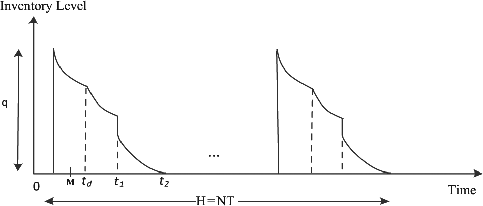
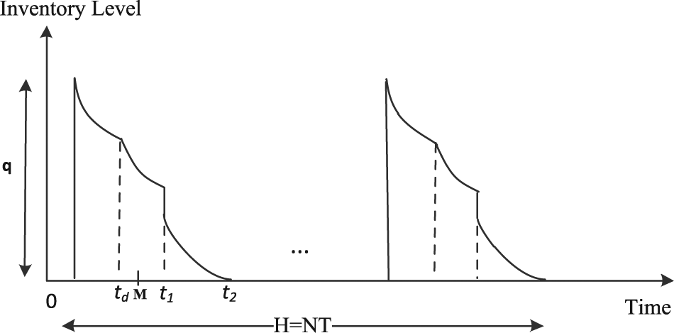
In this model, the items are produced at the beginning of the period which contains defective items of $α$ percent with a known pdf of $f (α)$ . As mentioned above, the first-stage inspection of the manufacturer makes inspection errors. According to the Type 2 inspection error, $α γ Q_{1 m}$ units of produced items during $[0, t_{1}]$ are falsely regarded as serviceable items that the retailer distinguishes them in one-stage inspection process. Here, the retailer model is described as follows. During the time interval [0, $t_{d}$ ], the inventory level decreases due to demand only. At time $t_{d}$ , deterioration starts, and thus, during the interval [ $t_{d}, t_{1}$ ], the inventory level decreases due to the demand and deterioration. Subsequently, the inventory level drops to 0 due to both demand and deterioration during the time interval $[t_{1}, t_{2}]$ (see Figures 1 and 2). The model’s details are given in Appendix 1.

Figure 1.

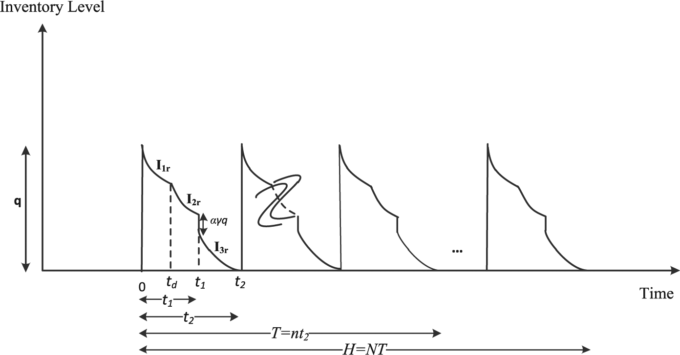
Graphical representation of the retailer’s inventory system.

Figure 2.

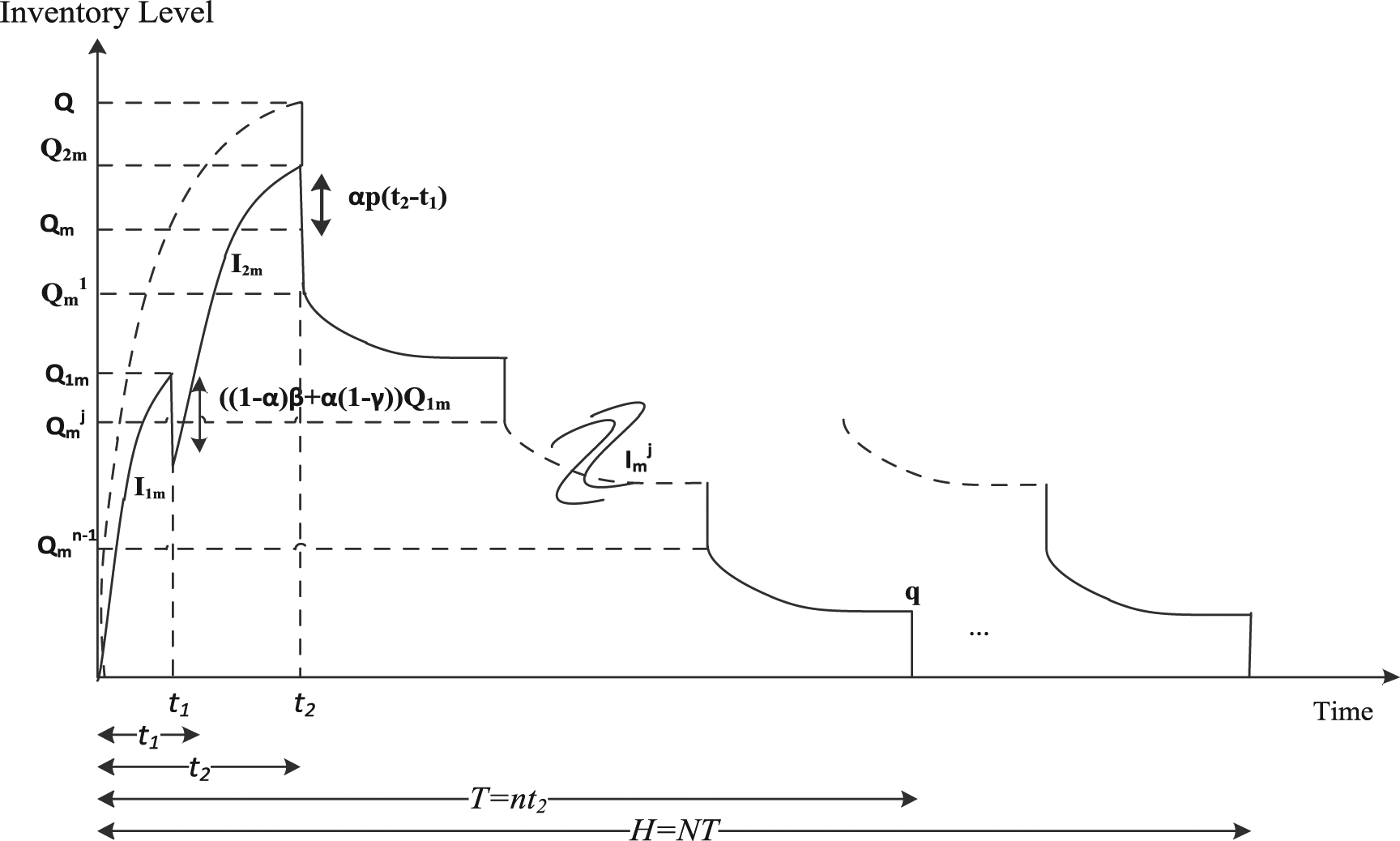
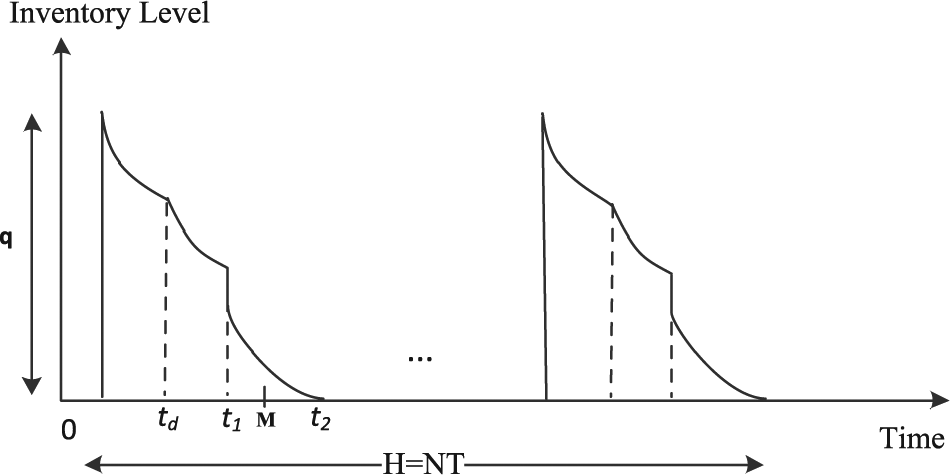
Behavior of the inventory level for the manufacturer.

Now, the presented value of inventory costs can be obtained as follows:

1. The present worth of the ordering cost.

Since the ordering cost in each cycle time is done at the beginning of each cycle T, the present value of ordering cost for the first cycle is k, which is a constant value

OC = k

(1)

2. The present worth of the inspection cost.

The present worth of the inspection cost occurs during the time interval $[0, t_{1}]$ . According to Taheri-Tolgari et al.,²⁹ we assume it is at the middle of $t_{1}$ and can be expressed as

IC = sq \cdot e^{- (\frac{1}{2}) \cdot r \cdot t_{1}}

(2)

3. The present worth of the purchasing cost.

We assume this cost occurs at the beginning of $t_{2}$

PC = c_{1} q

(3)

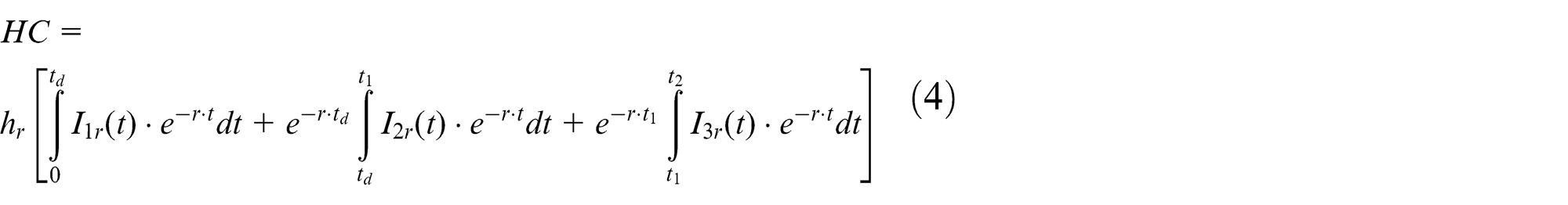
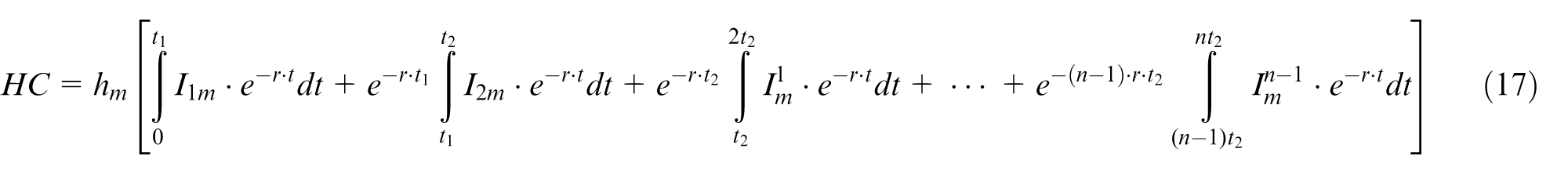
4. The present worth of the holding cost.

The present worth of the holding cost is given as follows

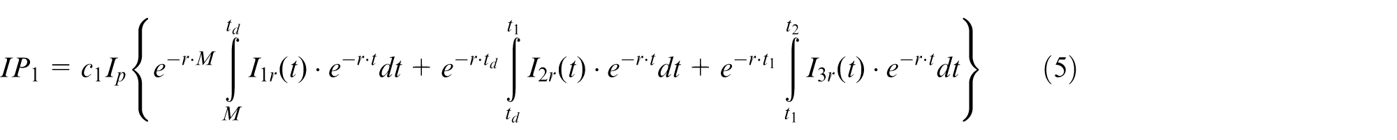
\begin{matrix} HC = \\ h_{r} [\int_{0}^{t_{d}} I_{1 r} (t) \cdot e^{- r \cdot t} dt + e^{- r \cdot t_{d}} \int_{t_{d}}^{t_{1}} I_{2 r} (t) \cdot e^{- r \cdot t} dt + e^{- r \cdot t_{1}} \int_{t_{1}}^{t_{2}} I_{3 r} (t) \cdot e^{- r \cdot t} dt] \end{matrix}

(4)

5. The present value of interest payable.

We consider the cases where the length of the credit period is longer or shorter than $t_{d}$ and $t_{1}$ .

Thus, we calculate the present value of interest payable for the items kept in stock under the following three cases.

Case 1: the delay time of payments occurs before deteriorating time or $0 < M \leq t_{d}$ (see Figure 3).

In this case, payment for the items is settled and the retailer starts paying the interest charged for all unsold items in inventory with rate $I_{p}$ . Thus, the present value of interest payable during [0, t ₂], is given as follows

\begin{matrix} I P_{1} = c_{1} I_{p} {e^{- r \cdot M} \int_{M}^{t_{d}} I_{1 r} (t) \cdot e^{- r \cdot t} dt + e^{- r \cdot t_{d}} \int_{t_{d}}^{t_{1}} I_{2 r} (t) \cdot e^{- r \cdot t} dt + e^{- r \cdot t_{1}} \int_{t_{1}}^{t_{2}} I_{3 r} (t) \cdot e^{- r \cdot t} dt} \end{matrix}

(5)

Case 2: the delay time of payments occurs after deteriorating time and before inspection time, that is, $t_{d} < M \leq t_{1}$ (see Figure 4).

The conditions of this case are similar to those for Case 1. Therefore, the present value of interest payable during [0, t ₂] is given as follows

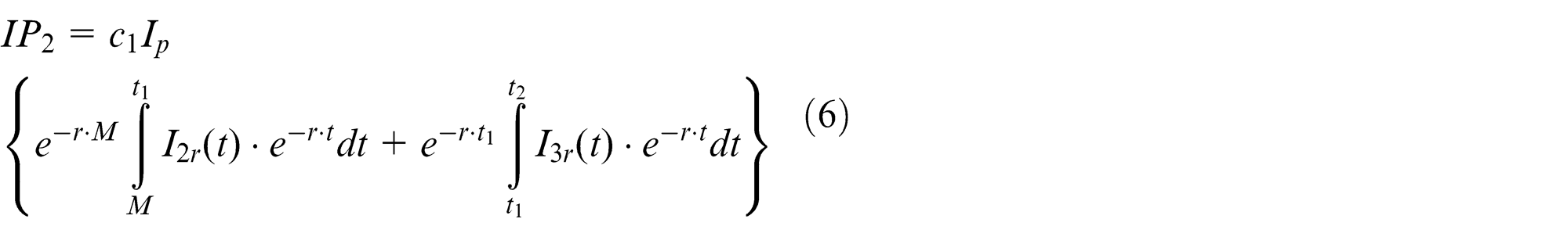
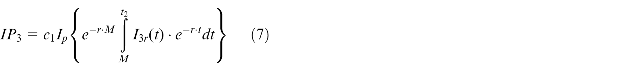
\begin{matrix} I P_{2} = c_{1} I_{p} \\ {e^{- r \cdot M} \int_{M}^{t_{1}} I_{2 r} (t) \cdot e^{- r \cdot t} dt + e^{- r \cdot t_{1}} \int_{t_{1}}^{t_{2}} I_{3 r} (t) \cdot e^{- r \cdot t} dt} \end{matrix}

(6)

Case 3: the delay time of payments occurs after inspection time and before the replenishment time or $t_{1} < M \leq t_{2}$ (see Figure 5).

In this case, the retailer starts paying the interest for the items in stock from time M to $t_{2}$ with rate $I_{p}$ . Hence, the present value of interest payable during [0, t ₂] is as given below

I P_{3} = c_{1} I_{p} {e^{- r \cdot M} \int_{M}^{t_{2}} I_{3 r} (t) \cdot e^{- r \cdot t} dt}

(7)

Figure 3.

Case 1, $0 < M \leq t_{d}$ .

Figure 4.

Case 2, $t_{d} < M \leq t_{1}$ .

Figure 5.

Case 3, $t_{1} < M \leq t_{2}$ .

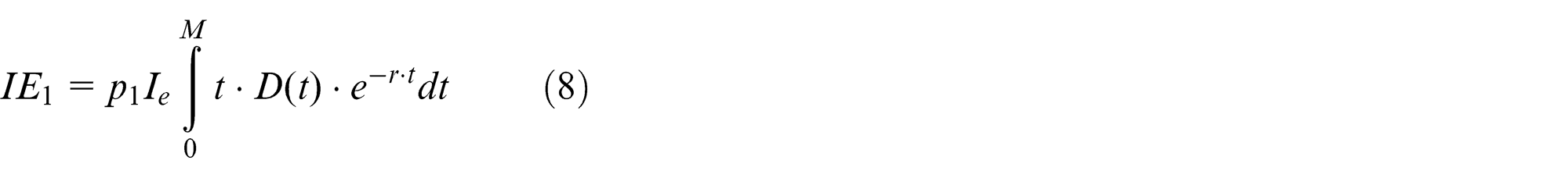
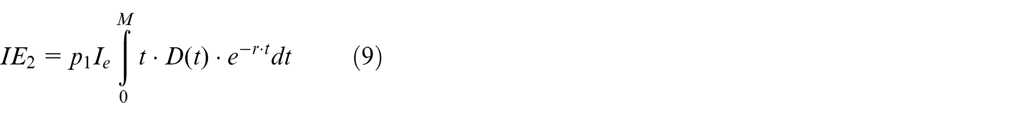
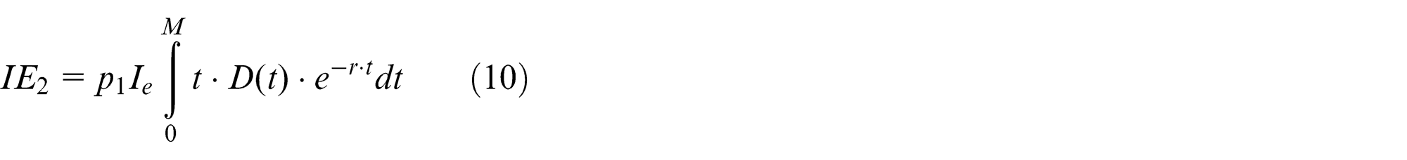
1. The present value of the interest earned.

There are different ways to calculate the interest earned. Here, the approach used by Geetha and Uthayakumar³⁰ is applied. We assume that during the time when the account is not settled, the retailer sells the goods and continues to accumulate sales revenue and earns interest with rate $I_{e}$ . Therefore, the interest earned during each [0, t ₂] is as follows for the three different cases:

Case 1: the delay time of payments occurs before deteriorating time or $0 < M \leq t_{d}$

I E_{1} = p_{1} I_{e} \int_{0}^{M} t \cdot D (t) \cdot e^{- r \cdot t} dt

(8)

Case 2: the delay time of payments occurs after deteriorating time and before production period time, that is, $t_{d} < M \leq t_{1}$

I E_{2} = p_{1} I_{e} \int_{0}^{M} t \cdot D (t) \cdot e^{- r \cdot t} dt

(9)

Case 3: the delay time of payments occurs after production period time and before duration of inventory cycle or $t_{1} < M \leq t_{2}$

I E_{2} = p_{1} I_{e} \int_{0}^{M} t \cdot D (t) \cdot e^{- r \cdot t} dt

(10)

Therefore, the present value of the retailer’s total cost over finite planning horizon, denoted by $T C_{r} (t_{1}, t_{2}, T, N)$ , is given by

\begin{matrix} T C_{r} (t_{1}, t_{2}, T, N) = {\begin{matrix} \sum_{i = 0}^{N} (OC + \sum_{0}^{n} (IC + PC + HC + I P_{1} - I E_{1}) \cdot e^{- r \cdot i \cdot t_{2}}) \cdot e^{- r \cdot i \cdot T} 0 < M \leq t_{d} \\ \sum_{i = 0}^{N} (OC + \sum_{0}^{n} (IC + PC + HC + I P_{2} - I E_{2}) \cdot e^{- r \cdot i \cdot t_{2}}) \cdot e^{- r \cdot i \cdot T} t_{d} < M \leq t_{1} \\ \sum_{i = 0}^{N} (OC + \sum_{0}^{n} (IC + PC + HC + I P_{3} - I E_{3}) \cdot e^{- r \cdot i \cdot t_{2}}) \cdot e^{- r \cdot i \cdot T} t_{1} < M \leq t_{2} \end{matrix} \end{matrix}

(11)

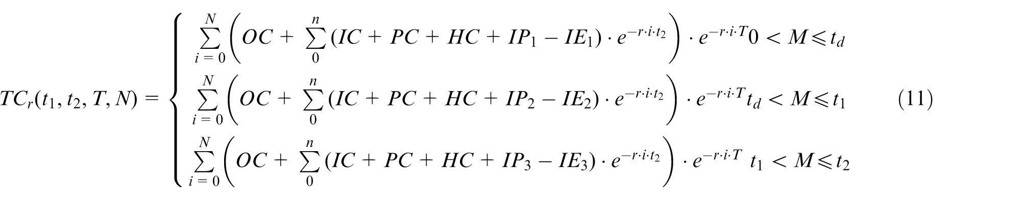
The value of the variables $t_{2}$ and T can be replaced by the equations $T = H / N$ and $t_{2} = T / n$ and we will use the geometric series formula for $\sum_{i = 0}^{n} e^{- r \cdot i \cdot t_{2}} = (1 - e^{- r \cdot n \cdot t_{2}}) / (1 - e^{- r \cdot t_{2}})$ and $\sum_{i = 0}^{N} e^{- r \cdot i \cdot T} = (1 - e^{- r \cdot N \cdot T}) / (1 - e^{- r \cdot T})$ . Therefore, the objective of this article is to find the variables of $t_{1}$ and N that minimize $T C_{r} (t_{1}, N)$ subject to $0 \leq t_{1} \leq t_{2}$ . Since $α$ , $β$ and $γ$ are the random variables with known $pdf$ of $f (α)$ , $f (β)$ and $f (γ)$ , the expressed value of $T C_{r}$ , that is, $ET C_{r}$ , becomes

MinET C_{r} (t_{1}, N) st : 0 \leq t_{1} \leq t_{2}

(12)

Manufacturer’s model

The manufacturer uses the delay equal-sized shipment policy. The inspection of the manufacturer consists of two stages in which the first stage contains inspection errors. After the inspection process, the items are dispatched to the retailer in n equal size shipments that contain $α γ$ percent of defective items. During the production cycle, the change in the inventory level of each finished item is influenced by production and deterioration and is given in Appendix 2.

In the non-production cycle, the change in the inventory level is affected by deterioration and is given in Appendix 3.

The present worth of the individual costs during first cycle of $[0, T]$ is given as follows:

1. The present worth of the setup cost.

Since setup cost in each cycle time is done at the beginning of each cycle, the present value of that is x for each cycle T, which is a constant value

SC = x .

(13)

2. The present worth of the producing cost.

We assume this cost occurs at the beginning of $t_{2}$

PC = cQ .

(14)

3. The present worth of the inspection cost.

The present worth of the first inspection stage cost occurs during the time interval [0, t ₁]. According to Taheri-Tolgari et al.,²⁹ we assume it is at the middle of $t_{1}$ and can be expressed as

IC 1 = s_{1} Q_{1} \cdot e^{- (\frac{1}{2}) \cdot r \cdot t_{1}}

(15)

For the second stage

IC 2 = s_{2} p (t_{2} - t_{1}) \cdot e^{- (\frac{1}{2}) \cdot r \cdot t_{2}}

(16)

4. The present worth of the holding cost

\begin{matrix} HC = h_{m} [\int_{0}^{t_{1}} I_{1 m} \cdot e^{- r \cdot t} dt + e^{- r \cdot t_{1}} \int_{t_{1}}^{t_{2}} I_{2 m} \cdot e^{- r \cdot t} dt + e^{- r \cdot t_{2}} \int_{t_{2}}^{2 t_{2}} I_{m}^{1} \cdot e^{- r \cdot t} dt + \dots + e^{- (n - 1) \cdot r \cdot t_{2}} \int_{(n - 1) t_{2}}^{n t_{2}} I_{m}^{n - 1} \cdot e^{- r \cdot t} dt] \end{matrix}

(17)

5. The present worth of the opportunity interest loss

The present worth of the manufacturer’s opportunity interest loss is given by

IL = \sum_{i = 0}^{n} c_{1} I_{s} q \cdot e^{- r \cdot M} \cdot e^{- r \cdot i \cdot t_{2}}

(18)

6. The present worth of the inspection error cost.

It includes the lost profit of the items that are falsely screened as defective items and removed from the inventory level. It is assumed that the inspection error cost occurs at the end of $t_{1}$ and it can be derived as

EC = (1 - α) β Q_{1} c_{1} \cdot e^{- r \cdot t_{1}}

(19)

It is assumed that all these costs occur once in each cycle. Thus, the present worth of the total cost includes setup cost $(SC)$ , producing cost $(PC)$ , screening cost $(IC 1 + IC 2)$ , holding cost $(HC)$ , opportunity interest loss $(IL)$ and inspection error cost $(EC)$ . Also, delivery to the retailer starts from the duration $[t_{2}, 2 t_{2}]$ , and as a result, the manufacturer does not deposit the opportunity interest loss for duration [0, t ₂]. Therefore, the present value of the manufacturer’s total cost over finite planning horizon, denoted by $T C_{r} (t_{1}, t_{2}, T, N)$ , is as follows

\begin{matrix} T C_{m} (t_{1}, t_{2}, T, N) = \\ \sum_{i = 0}^{N} (SC + PC + I C_{1} + I C_{2} + HC + IL + EC) \cdot \\ e^{- r \cdot i \cdot T} - c_{1} I_{s} q \cdot e^{- r \cdot M} \end{matrix}

(20)

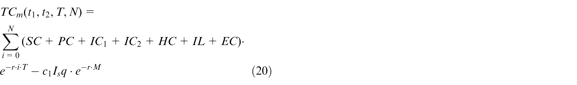
We want to minimize $T C_{m}$ subject to the following constraints

0 \leq t_{1} \leq t_{2} and N \in N

Equation (42) is composed of $t_{1}$ , $t_{2}$ , T and N variables with a high complexity. We can reduce the number of variables by relations of $T = H / N$ and $t_{2} = T / n$ and also the geometric series formula for $\sum_{i = 0}^{N} e^{- riT} (1 - e^{- rNT}) / (1 - e^{- rT})$ . Thus, the objective function consists of two variables, $t_{1}$ and N. Since $α$ , $β$ and $γ$ are the random variables with known $pdf$ of $f (α)$ , $f (β)$ and $f (γ)$ , the expressed value of $T c_{m}$ , that is, $ET C_{m}$ , becomes

MinET C_{m} (t_{1}, N) st : 0 \leq t_{1} \leq t_{2}

(21)

Integrated policy

For the integrated policy, it is assumed that the business information between the retailer and the manufacturer can be shared. First, the sum of the cost of the manufacturer and the retailer is derived, then, based on this obtained cost, the optimal solution can be calculated

ETC (t_{1}, N) = ET C_{r} (t_{1}, N) + ET C_{m} (t_{1}, N)

(22)

To find the optimal number of cycles, we calculate the objective function for several N. Also, in order to determine the optimal value of $t_{1}$ , we calculate the derivative of objective function by variable $t_{1}$ and let it equal to 0

\frac{\partial ETC}{\partial t_{1}} = 0

(23)

Optimal solution procedure

We have used the following algorithm to obtain the optimal amount of N and $t_{1}$ for Case 1, $0 < M \leq t_{d}$ .

Step 1. Let $N = 1$ .

Step 2. Take the partial derivatives of $ETC (t_{1}, N)$ with respect to $t_{1}$ and equate the results to 0. Then calculate the $ETC$ .

Step 3. Add one unit to N and repeat Step 2 for new N. If there is no decrease in the new $ETC$ , then show the previous one which has the minimum value.

The necessary condition for minimizing $ETC (t_{1}, N)$ for a given positive integer of N is

\frac{\partial ETC}{\partial t_{1}} = 0

(24)

The sufficient condition below can satisfy the concavity of objective function

\frac{\partial^{2} ETC}{\partial^{2} t_{1}} > 0

(25)

Since ETC is a very complicated function due to high-power expression of the exponential function, we can assess it numerically in the following illustrative example. The flow chart of the solution procedure is shown in Figure 6.

Figure 6.

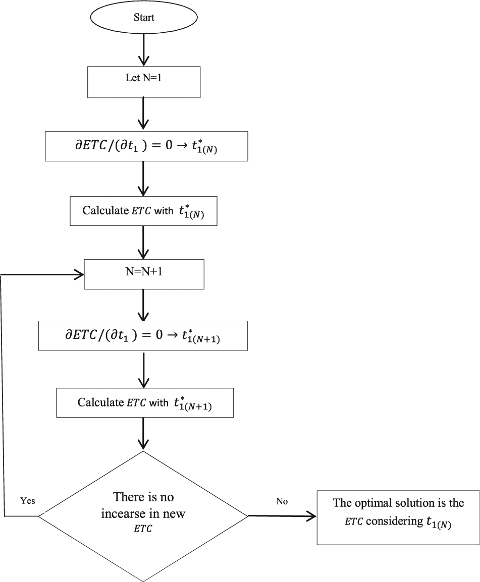
Flow chart of the solution procedure.

Numerical example

The preceding algorithm can be illustrated using the numerical example. The results can be found by applying the Maple 16. The parameters of the numerical example are as follows

D (t) = a + bt = 100 + 60 t

$θ = 0.18$

$c_{1} = $ 60 / per unit / per unit time$

c = $20/per unit/per unit time

$h_{r} = $ 4 / per unit / per unit time$

p = 100 units/per unit time

A = $300/per order

$α ~ u (0, 0.04)$

$β ~ u (0.03, 0.05)$

$γ ~ u (0.04, 0.06)$

µ = 337 units/per unit time

s = $1/per unit/per unit time

s ₁ = 0.5/per unit/per unit time

s ₂ = 0.5/per unit/per unit time

X = $500/per production cycle

$h_{m} = $ 9 / per unit / per unit time$

r = 0.04

H = 10 unit time

n = 4 delivery number/per order

$p_{1} = 70$

$I_{p} = 0.06$

$I_{e} = 0.03$

$I_{s} = 0.03$

$M = 0.1$

$t_{d} = 0.2$

f (α) = {\begin{matrix} 25, 0 \leq α \leq 0.04 \\ 0, otherwise \end{matrix}

f (β) = {\begin{matrix} 50, 0.03 \leq β \leq 0.05 \\ 0, otherwise \end{matrix}

f (γ) = {\begin{matrix} 50, 0.04 \leq γ \leq 0.06 \\ 0, otherwise \end{matrix}

From Table 2, if all the conditions and constraints are satisfied, the optimal solution can be derived. In this example, the minimum present value of total cost of supply chain is found in the third cycle. Therefore, the optimal solution is as follows: $t_{1}^{*} = 0.5242$ , $N^{*} = 3$ , $t_{2}^{*} = 0.84$ , $Q_{2 m}^{*} = 30.911$ and $Q_{m}^{*} = 30.911$ .

Table 2.

Optimal solution of the numerical example.

N	ETC	$ET C_{r}$	$ET C_{m}$	Q	$Q_{2 m}$	$Q_{m}$	$t_{1}$	$t_{2}$
2	185535.315	107320.279	78215.035	199.718	108.851	62.291	0.6271	1.25
3^a	182903.064^a	114579.116^a	68323.947^a	115.633^a	74.631^a	30.911^a	0.5242^a	0.84^a
4	194464.643	127622.291	66842.353	80.591	56.547	15.238	0.4726	0.625

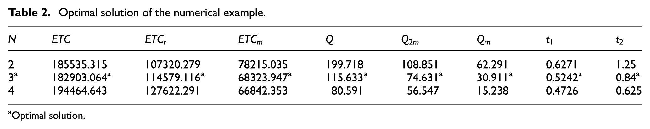
Optimal solution.

By substituting the optimal values of $N^{*}$ and $t_{1}^{*}$ in Equation (25), it will be shown that ETC is strictly concave

\frac{\partial^{2} ETC}{\partial^{2} t_{1}} = 130328.6801

If parameter A reduces, the optimal $N^{*}$ increases. It causes more total cost. We consider the change in parameter A in the next section.

Sensitivity analysis

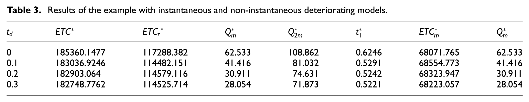
Now, we investigate the impact of parameters on the optimal solution of the model. First, we discuss the effect of instantaneous and non-instantaneous deteriorating items on the optimal solution. With the instantaneous deteriorating rate, the expected value of the total cost of the whole supply chain increases. It means that if the situation of stock improved, the whole cost of the system is decreased (see Table 3).

Table 3.

Results of the example with instantaneous and non-instantaneous deteriorating models.

$t_{d}$	$ET C^{*}$	$ET {C_{r}}^{*}$	$Q_{m}^{*}$	$Q_{2 m}^{*}$	$t_{1}^{*}$	${ETC}_{m}^{*}$	$Q_{m}^{*}$
0	185360.1477	117288.382	62.533	108.862	0.6246	68071.765	62.533
0.1	183036.9246	114482.151	41.416	81.032	0.5291	68554.773	41.416
0.2	182903.064	114579.116	30.911	74.631	0.5242	68323.947	30.911
0.3	182748.7762	114525.714	28.054	71.873	0.5221	68223.057	28.054

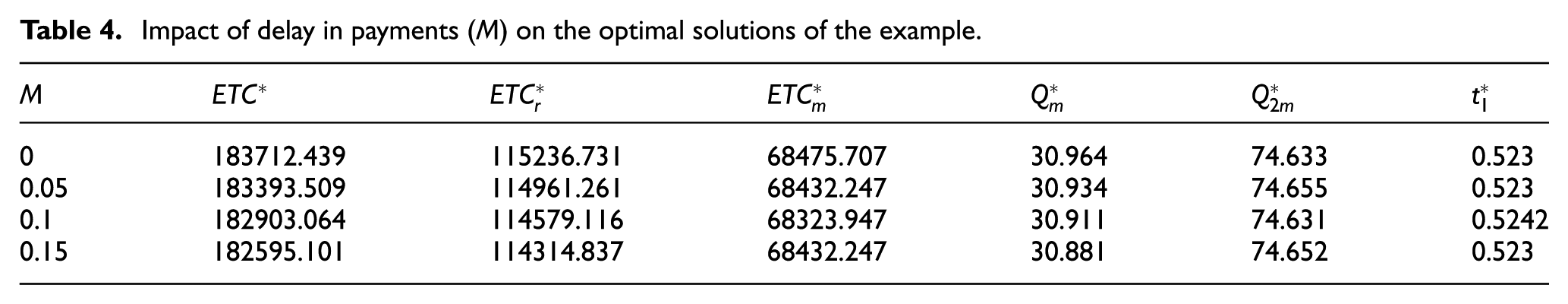
If the manufacturer does not consider the delay in payments (M = 0), the expected value of the total cost of the whole supply chain increases. As a result, if the retailers wish to increase their profit, they should try to get credit periods for their payments (see Table 4).

Table 4.

Impact of delay in payments (M) on the optimal solutions of the example.

M	$ET C^{*}$	${ETC}_{r}^{*}$	${ETC}_{m}^{*}$	$Q_{m}^{*}$	$Q_{2 m}^{*}$	$t_{1}^{*}$
0	183712.439	115236.731	68475.707	30.964	74.633	0.523
0.05	183393.509	114961.261	68432.247	30.934	74.655	0.523
0.1	182903.064	114579.116	68323.947	30.911	74.631	0.5242
0.15	182595.101	114314.837	68432.247	30.881	74.652	0.523

The numerical results of Tables 3 and 4 are summarized in Figures 7 and 8, respectively.

Figure 7.

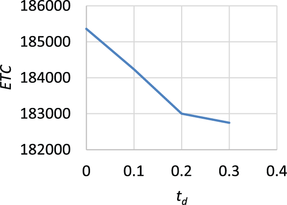
Numerical results of Table 3 which include the impact of instantaneous and non-instantaneous deteriorating models on ETC.

Figure 8.

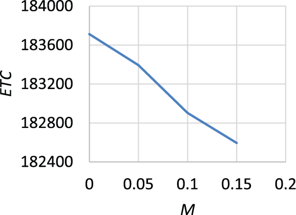
Numerical results of Table 4 which include the impact of delay in payments (M) on ETC.

Third, we investigate the effect of the changes in the value of a, b, $I_{p}$ , $I_{s}$ , r, $α$ , $β$ , $γ$ , $h_{r}$ , $h_{m}$ on the $ETC$ , $ET C_{r}$ , $ET C_{m}$ , $t_{1}$ and q (Table 5).

Table 5.

Sensitivity analysis results.

Parameter	% Change in parameter	$ET C^{*}$	${ETC}_{r}^{*}$	${ETC}_{m}^{*}$	$t_{1}^{*}$	$q^{*}$	$Q_{2 m}^{*}$	$Q_{m}^{*}$	$N^{*}$
A	−50	213518.072	88841.653	35461.432	0.526	60.221	74.763	50.261	7
	−25	187639.0921	732912.001	54761.442	0.633	94.612	75.8743	25.764	5
	25	139832.075	451973.023	64291.327	0.7825	148.04	76.173	43.452	3
	50	116452.916	231894.874	89211.543	0.8910	274.52	110.519	89.642	2
a	−50	120560.947	67100.726	53460.221	0.793	69.611	73.112	3.991	3
	−25	150761.828	89815.286	60946.541	0.633	92.622	74.023	19.991	3
	25	216133.998	140504.491	75629.507	0.448	138.64	75.045	38.497	3
	50	247937.061	151646.476	96290.585	0.503	271.61	109.485	74.644	2
b	−50	159222.076	98791.64943	60430.427	0.434	171.75	109.836	81.586	2
	−25	171935.483	102623.676	69311.806	0.537	185.73	109.313	71.258	2
	25	194507.180	118139.691	76367.491	0.607	121.53	74.169	22.599	3
	50	206952.068	122610.227	84341.841	0.678	127.42	73.769	15.477	3
$I_{p}$	−50	181825.709	113666.729	68158.979	0.520	115.63	74.676	31.326	3
	−25	182408.321	114149.271	68259.049	0.522	115.63	74.665	31.114	3
	25	183575.233	115124.414	68450.819	0.526	115.63	74.643	30.706	3
	50	184159.399	115616.657	68542.742	0.528	115.63	74.632	30.509	3
$I_{s}$	−50	165333.863	128239.798	37094.065	0.194	115.63	76.402	63.895	3
	−25	172801.575	120356.888	52444.687	0.396	115.63	75.344	43.699	3
	25	194651.148	110360.497	84290.651	0.612	115.63	74.168	22.091	3
	50	207192.585	107065.457	100127.128	0.676	115.63	73.809	15.645	3
r	−50	199302.461	125321.474	73980.987	0.518	115.63	74.664	31.531	3
	−25	190844.393	119778.197	71066.196	0.521	115.63	74.647	31.215	3
	25	175442.726	109700.129	65742.597	0.527	115.63	74.614	30.616	3
	50	168430.245	105118.891	63311.355	0.530	115.63	74.598	30.332	3
$α$	−50	182821.1248	114522.757	68298.367	0.524	114.27	75.061	30.912	3
	−25	182862.064	114550.911	68311.153	0.524	114.94	74.845	30.911	3
	25	182944.079	114607.329	68336.751	0.524	116.32	74.415	30.909	3
	50	182985.122	114635.561	68349.561	0.524	117.02	74.199	30.908	3
$β$	−50	182757.903	114679.849	68078.054	0.522	115.63	75.565	31.125	3
	−25	182830.407	114629.501	68200.907	0.523	115.63	75.099	31.018	3
	25	182975.869	114528.693	68447.175	0.525	115.63	74.159	30.803	3
	50	183048.854	114478.263	68570.591	0.526	115.63	73.687	30.695	3
$γ$	−50	182814.754	114523.118	68291.635	0.524	115.63	74.607	30.913	3
	−25	182858.888	114551.101	68307.787	0.524	115.63	74.618	30.912	3
	25	182947.276	114607.161	68340.115	0.524	115.63	74.642	30.909	3
	50	182991.474	114635.182	68356.291	0.524	115.63	74.654	30.908	3
$h_{r}$	−50	181350.415	113154.293	68196.122	0.521	115.63	74.672	74.672	3
	−25	182170.751	113893.298	68277.452	0.522	115.63	74.663	31.075	3
	25	183812.560	115379.811	68432.751	0.525	115.63	74.645	30.745	3
	50	184633.968	116127.036	68506.932	0.527	115.63	74.636	30.586	3
$h_{m}$	−50	173526.984	105503.241	68023.743	0.673	199.71	108.638	57.681	2
	−25	178413.977	113914.548	64499.428	0.539	115.63	74.571	29.381	3
	25	187599.048	115340.674	72258.374	0.509	115.63	74.736	32.419	3
	50	192236.319	116031.427	76204.892	0.494	115.63	74.817	33.915	3

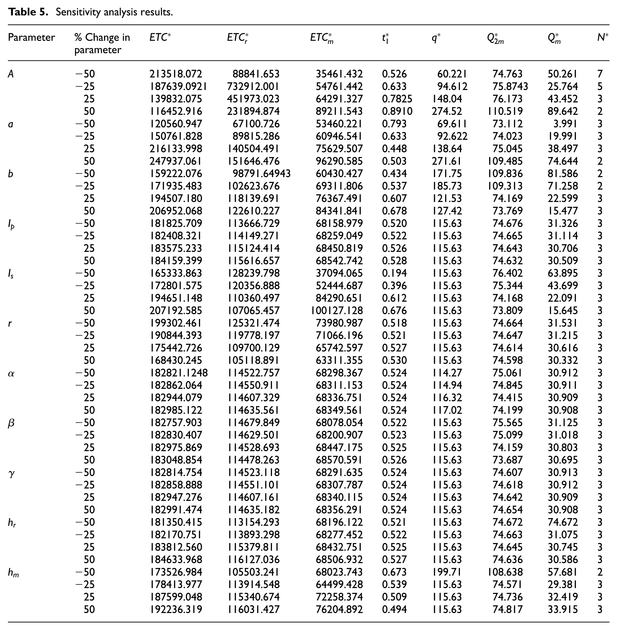
We investigate the effects of the changes in the value of parameters $a, b, I_{p}, I_{s}, r, α$ , $β$ , $γ$ , $h_{r}$ and $h_{m}$ on the $ET C^{*}, {ETC}_{r}^{*}$ , ${ETC}_{m}^{*}$ , $t_{1}^{*}$ , $q^{*}$ , $Q_{2 m}^{*}$ , $Q_{m}^{*}$ and $N^{*}$ based on the example. The sensitive analysis is performed by changing each value of the parameters by +50%, +25%, −25% and −50%, taking one parameter at a time end keeping the remaining parameter values changed. The computational results are shown in Table 3. The sensitive analysis shown in Table 3 indicates the following observations:

When the value of parameters a, b, $I_{p}$ , $I_{s}$ , $α$ , $γ$ , $h_{r}$ and $h_{m}$ increase (decrease), the value of $ETC$ will increase (decrease).

When the value of parameters M, r and $β$ increase (decrease), the value of $ETC$ will decrease (increase).

Conclusion

In this study, an integrated supply chain model for deteriorating items with permissible delay in payments, inflation, imperfect production process and inspection errors is considered. The demand is time-dependent. Also, it is assumed that the deterioration rate for the retailer is non-instantaneous. To the best of our knowledge, this is the first model in integrated supply chain policy models that considers delay in payments, inflation, deteriorating items, imperfect production process and inspection errors. We believe that the proposed model can provide more realistic and general results. The manufacturer has two stages of inspection. The first stage of the manufacturer’s inspection process contains two types of errors, one is that a defective item may be classified to be non-defective, while the other is that a non-defective item may be classified to be defective. The second stage is done at the end of the production period without inspection errors. As soon as the retailer receives the lot, a 100% inspection process of the lot is conducted, and the inspection process and demand proceed simultaneously. The proportion of defective items and the proportion of Type 1 and Type 2 inspection errors are assumed to be random variables.

The expected total cost of the manufacturer, the retailer and the integrated supply chain is derived and a solution procedure, free of using the convexity, is provided to find the optimal solution that minimizes the expected total integrated cost. A numerical example and sensitivity analyses are conducted to illustrate this procedure. Finally, this inventory model can further be extended by taking some features such as price-dependent demand rate, variable deterioration rate, shortages with full or partial backlogging, quantity discounts, multiple products, partial credit trade policy and two warehouses. Also, multi-vendors and multi-buyers’ supply chains and effect of the repair or replenishment of the deteriorated and imperfect items can be directed in future studies.

Footnotes

Appendix 1

The inventory level is affected by the demand during the time interval [0, t_d ]. Therefore, the differential equation, $I_{1 r} (t)$ is

(26)

\frac{d I_{1 r} (t)}{dt} = - D = - (a + bt) (0 \leq t \leq t_{d})

With the condition $I_{1 r} (0) = q$ , solving equation (26) yields

(27)

I_{1 r} (t) = - \frac{1}{2} {bt}_{d}^{2} - a t_{d} + q (0 \leq t \leq t_{d})

The inventory level is affected by the deterioration and demand during the time interval $[t_{d}, t_{1}]$ . Hence, the inventory status is as follows

(28)

\frac{d I_{2 r} (t)}{dt} + θ I_{2 r} (t) = - D = - (a + bt) (t_{d} \leq t \leq t_{1})

With the condition $I_{2 r} (t_{d}) = I_{1 r} (t_{d})$ , solving equation (28) yields

(29)

\begin{matrix} I_{2 r} (t) = - \frac{a}{θ} + \frac{b}{θ^{2}} - \frac{bt}{θ} \\ - \frac{e^{- θ t} (\frac{1}{2} {bt}_{d}^{2} + a t_{d} - q - \frac{a}{θ} + \frac{b}{θ^{2}} - \frac{b t_{d}}{θ})}{e^{- θ t_{d}}} (t_{d} \leq t \leq t_{1}) \end{matrix}

Thus, the differential equation below represents the inventory status during the time interval $[t_{1}, t_{2}]$

(30)

\frac{d I_{3 r} (t)}{dt} + θ I_{3 r} (t) = - D = - (a + bt) (t_{1} \leq t \leq t_{2})

With the condition $I_{3 r} (t_{1}) = I_{2 r} (t_{1}) - α γ q$ , solving equation (30) yields

(31)

\begin{matrix} I_{3 r} (t) = \frac{1}{2} \frac{1}{θ^{2} e^{- θ t_{d}} e^{- θ t_{1}}} \\ ((((- {bt}_{d}^{2} - 2 a t_{d} + 2 q) θ^{2} + (2 b t_{d} + 2 a) θ - 2 b) e^{- θ t} \\ - 2 ((a + bt) θ - b) e^{- θ t_{d}}) e^{- θ t_{1}} - 2 e^{- θ t} α γ q θ^{2} e^{- θ t_{d}} \end{matrix}) (t_{1} \leq t \leq t_{2})

At $t = t_{2}$ , $I_{3 r} (t) = 0$ , equation (31) gives order quantity as follows

(32)

\begin{matrix} q = \frac{1}{θ^{2} e^{- θ t} (e^{- θ t_{1}} - α γ e^{- θ t_{d}})} \end{matrix} (((t_{d} (\frac{1}{2} b t_{d} + a) θ^{2} + (- b t_{d} - a) θ + b) e^{- θ t} + e^{- θ t_{d}} ((a + bt) θ - b)) e^{- θ t_{1}})

Appendix 2

During the production cycle, the change in inventory level of each finished item is influenced by production and deterioration

(33)

\frac{d I_{1 m} (t)}{dt} + θ I_{1 m} (t) = p (0 \leq t \leq t_{1})

(34)

\frac{d I_{2 m} (t)}{dt} + θ I_{2 m} (t) = p (0 \leq t \leq t_{1})

With the condition $I_{1 m} (0) = 0$ , solving equation (33) yields

(35)

I_{1 m} (t) = \frac{p}{θ} (1 - e^{- θ \cdot t}) (0, \leq t \leq t_{1})

If we put t = t ₁ into I _1m(t), the production lot size of manufacturer at the end of the first inspection stage (Q _1m) will be obtained as follows

(36)

Q_{1 m} = \frac{p}{θ} (1 - e^{- θ \cdot t_{1}})

And the solution of the differential equation (34) along with the boundary condition, $t = t_{1}$ , $I (t) = I_{1 m} (t_{1}) - ((1 - α) β + α (1 - γ)) Q_{1 m}$ , is

(37)

\begin{matrix} I_{2 m} (t) = \frac{p}{θ} \\ - \frac{e^{- θ \cdot t} (\frac{- p + p \cdot e^{- θ \cdot t_{1}} + Q_{1 m} θ β - Q_{1 m} θ β α + Q_{1} θ α - Q_{1 m} θ α γ}{θ} + \frac{p}{θ})}{e^{- θ \cdot t_{1}}} \\ (t_{1} \leq t \leq t_{2}) \end{matrix}

If we put t = t ₂ into I _2m(t), the production lot size of manufacturer at the end of production cycle (Q _2m) will be obtained as follows

(38)

\begin{matrix} Q_{2 m} = \frac{p}{θ} \\ - \frac{e^{- θ \cdot t_{2}} (\frac{- p + p \cdot e^{- θ \cdot t_{1}} + Q_{1} θ β - Q_{1} θ β α + Q_{1} θ α - Q_{1} θ α γ}{θ} + \frac{p}{θ})}{e^{- θ \cdot t_{1}}} \end{matrix}

In addition, Q is the production size of the manufacturer without inspection processes and can be expressed as

(39)

Q = \frac{p}{θ} (1 - e^{- θ \cdot t_{2}})

The relationship between $Q_{m}^{1}$ , production lot size of the manufacturer at the beginning of non-production cycle, and $Q_{m}$ , production lot size of manufacturer at the end of production time after removing imperfect items in the second stage of inspection, is

(40)

Q_{m} = Q_{2 m} - p (t_{2} - t_{1}) α

Q_{m}^{1} = Q_{m} - q

Appendix 3

In the non-production cycle, the change in inventory level is affected by deterioration

(41)

\frac{{dI}_{m}^{j} (t)}{dt} + θ I_{m}^{j} (t) = 0 (t_{2} \leq t \leq n t_{2})

With boundary condition of $I_{m}^{j} (0) = Q_{m}^{j}$ , the inventory level is

(42)

I_{m}^{j} (t) = Q_{m}^{j} \cdot e^{- θ \cdot t} (t_{2} \leq t \leq n t_{2})

According to Figure 2

(43)

I_{m}^{j} (t_{2}) = Q_{m}^{n - 1} \cdot e^{- θ \cdot t_{2}} = q

(44)

Q_{m}^{n - 1} = q \cdot e^{θ \cdot t_{2}}

Also, the lot size at the beginning of cycle of n is 0

(45)

\begin{matrix} I_{m}^{n - 2} (0) = Q_{m}^{n - 2} = (q + Q_{m}^{n - 1}) \cdot e^{- θ \cdot t_{2}} \\ = q (e^{θ \cdot t_{2}} + {(e^{θ \cdot t_{2}})}^{2}) \end{matrix}

(46)

\begin{matrix} I_{m}^{j} (0) = Q_{m}^{j} = q (e^{θ \cdot t_{2}} + \dots + {(e^{θ \cdot t_{2}})}^{j}) \\ = q \cdot e^{θ \cdot t_{2}} (\frac{1 - {(e^{θ \cdot t_{2}})}^{n - j}}{1 - e^{θ \cdot t_{2}}}) \end{matrix}

Declaration of conflicting interests

The author(s) declared no potential conflicts of interest with respect to the research, authorship and/or publication of this article.

Funding

The author(s) received no financial support for the research, authorship and/or publication of this article.

References

Goyal

. An integrated inventory model for a single supplier-single customer problem. Int J Prod Res 1976; 15: 107–111.

Wee

Huang

. An integrated production-inventory model with imperfect production processes and Weibull distribution deterioration under inflation. Int J Prod Econ 2007; 106: 248–260.

Yan

Banerjee

Yang

. An integrated production–distribution model for a deteriorating inventory item. Int J Prod Econ 2011; 133: 228–232.

Moussawi-Haidar

Dbouk

Jaber

et al . Coordinating a three-level supply chain with delay in payments and a discounted interest rate. Comput Ind Eng 2014; 69: 29–42.

Goyal

. Economic order quantity under conditions of permissible delay in payments. J Oper Res Soci 1985; 36: 335–338.

Ouyang

Ynag

. A study on an inventory model for non-instantaneous deteriorating items with permissible delay in payments. Comput Ind Eng 2006; 51(4): 637–651.

Liu

. Optimal replenishment policy for the EPQ model with permissible delay in payments and allowable shortages. Appl Math Model 2010; 34: 3108–3117.

Maihami

Nakhai Kamal Abadi

. Joint control of inventory and its pricing for non-instantaneously deteriorating items under permissible delay in payments and partial backlogging. Math Comput Model 2012; 55: 1722–1733.

Jana

Maity

Roy

. A three-layer supply chain integrated production-inventory model under permissible delay in payments in uncertain environments. J Uncertain Anal Appl 2013; 1: 6.

10.

Chern

Chan

Teng

et al . Nash equilibrium solution in a vendor–buyer supply chain model with permissible delay in payments. Comput Ind Eng 2014; 70: 116–123.

11.

Buzacott

. Economic order quantity with inflation. Oper Res Quart 1975; 26: 553–558.

12.

Sarker

Jamal

AMM

Wang

. Supply chain models for perishable products under inflation and permissible delay in payment. Comput Oper Res 2000; 27: 59–75.

13.

Sarkar

Moon

. An EPQ model with inflation in an imperfect production system. Appl Math Comput 2011; 217: 6159–6167.

14.

Guria

Das

Mondal

et al . Inventory policy for an item with inflation induced purchasing price, selling price and demand with immediate part payment. Appl Math Model 2013; 37: 240–257.

15.

Ghoreishi

Mirzazadeh

Weber

. Optimal pricing and ordering policy for non-instantaneous deteriorating items under inflation and customer returns. Optimization. Epub ahead of print 18 November 2014. DOI: 10.1080/02331934.2013.853059.

16.

Ghoreishi

Mirzazadeh

Nakhai-Kamalabadi

. Optimal pricing and lot-sizing policies for an economic production quantity model with non-instantaneous deteriorating items, permissible delay in payments, customer returns, and inflation. Proc IMechE, Part B: J Engineering Manufacture. Epub ahead of print 29 April 2014. DOI: 10.1177/0954405414522215.

17.

Ghare

Schrader

. A model for exponentially decaying inventory. J Ind Eng 1963; 14: 238–243.

18.

Skouri

Konstantaras

Papachristos

et al . Inventory models with ramp type demand rate, partial backlogging and Weibull deterioration rate. Eur J Oper Res 2009; 192: 79–92.

19.

Das

Kar

Roy

et al . Two-warehouse production model for deteriorating inventory items with stock-dependent demand under inflation over a random planning horizon. Cent Europ J Oper Re 2012; 20(2): 251–280.

20.

Wee

Widyadana

. A production model for deteriorating items with stochastic preventive maintenance time and rework process with FIFO rule. Omega 2014; 41: 941–954.

21.

Sicilia

Rosa

MGDL

Acosta

et al . An inventory model for deteriorating items with shortages and time-varying demand. Int J Prod Econ. Epub ahead of print 8 April 2014. DOI: 10.1016/j.ijpe.2014.01.024.

22.

Rosenblatt

Lee

. Economic production cycles with imperfect production processes. IIE Trans 1986; 18: 48–55.

23.

Goyal

Huang

Chen

. A simple integrated production policy of an imperfect item for vendor and buyer. Prod Plan Control 2003; 14(7): 596–602.

24.

Khan

Jaber

Bonney

. An economic order quantity (EOQ) for items with imperfect quality and inspection errors. Int J Prod Econ 2011; 133: 113–118.

25.

Sana

. A production-inventory model of imperfect quality products in a three-layer supply chain. Decis Support Syst 2011; 50(2): 539–547.

26.

Yoo

Kim

Park

. Economic production quantity model with imperfect-quality items, two-way imperfect inspection and sales return. Int J Prod Econ 2009; 121: 255–265.

27.

Yoo

Kim

Park

. Inventory models for imperfect production and inspection processes with various inspection options under one-time and continuous improvement investment. Comp Oper Res 2012; 39(9): 2001–2015.

28.

Lee

Kim

. An optimal policy for a single-vendor single-buyer integrated production–distribution model with both deteriorating and defective items. Int J Prod Econ 2014; 147: 161–170.

29.

Taheri-Tolgari

Mirzazadeh

Jolai

. An inventory model for imperfect items under inflationary conditions with considering inspection errors. Comput Math Appl 2012; 63: 1007–1019.

30.

Geetha

Uthayakumar

. Economic design of an inventory policy for non-instantaneous deteriorating items under permissible delay in payments. J Comput Appl Math 2010; 233: 2492–2505.

An integrated supply chain model for deteriorating items considering delay in payments,imperfect quality and inspection errors under inflationary conditions

Abstract

Keywords

Introduction

Literature review

Methodology and model building

Notations

Assumptions

Model description

Non-integrated policy

Retailer’s model

Manufacturer’s model

Integrated policy

Optimal solution procedure

Numerical example

Sensitivity analysis

Conclusion

Footnotes

Appendix 1

Appendix 2

Appendix 3

Declaration of conflicting interests

Funding

References