An integrated systematic investigation of the process variables on surface generation in abrasive flow machining of titanium alloy 6Al4V

Abstract

This article presents an integrated and systematic investigation into the interaction and effects of the abrasive flow machining factors, through its three major process variables of the media velocity, temperature and quantity, which play an essential role in interfacing the ‘machine’ with ‘workpiece’ and ‘media’ corners of the abrasive flow machining triangle. The article also presents predictive models, main effects and industrially useful rule-of-thumb tools. Collectively, these variables offer machine operators the ability to manipulate the process behaviour when the opportunity to modify geometry and media levels is unavailable. In the media and geometry corners of the triangle, capital expenditure is required to adjust levels, making them economically and temporally limiting. The machine adjustments are physically limited by the hardware in use; however, this research finds that the range of response magnitude can vary significantly among the three process outcomes studied, that is, surface roughness, material removal and peak height reduction. Using a standard media and testpiece set-up, data are collected using a 3³ full factorial experiment design and translated into a response surface design (Box–Behnken) for predictive model development. Application to oil and gas industry parts is shown whereby data are utilised to aid in the abrasive flow machining of production parts.

Introduction

Modern high-value manufacturing (HVM) can be characterised by prolific use of high-performance materials, <5 µm tolerances, costly machine–tool combinations and geometrical complexity of components and products. In many industries, in particular the oil and gas and automotive sectors, primary manufacturing methods (turning, drilling and milling) are frequently insufficient to manufacture geometry and complexity to customer specifications. These requirements stem from miniaturisation (increasing the feature set a product can offer) and design freedom offered by the capability of nontraditional material removal (MR) methods (additive layer manufacturing (ALM), electro-discharge machining (EDM), electrochemical machining (ECM) and laser-based methods).^1–4 The additional capability awarded by nontraditional methods brings their own inherent issues, the most predominant of which is feature inaccessibility, followed by difficult- or impossible-to-inspect features and third, by availability of sufficiently capable part-finishing techniques (i.e. where grinding and manual deburring may be inappropriate).^4,5

In this light, we present abrasive flow machining (AFM) – the reciprocal pumping of an abrasive-laden slurry (∼50–1200 Pa/s at ∼10–200 bar) throughout an engineering component for the purpose of surface finishing, edge rounding, honing and removal of recast layer. The process is widely considered a ‘black art’ and while generally accepted by high-profile large enterprise (LE) manufacturers with high part volumes, establishing a presence within the high-value low-quantity world of Small to Medium Enterprise (SME) high added-value (HAV) manufacturing has proven difficult. Key reasons for this include high capital costs through machinery, consumables (media) and fixturing costs and battling currently accepted attitudes towards the process. ⁴ The overwhelming factor in process uptake is process knowledge – with no fixed axes and a ‘liquid cutting tool’, potential users assume that operating an AFM machine can be as simple as pumping media through their workpiece. The truth is far more complex, as illustrated in Figure 1, the triangle concept illustrated describes the three corners of the process and aims to identify each element within the corner.

Figure 1.

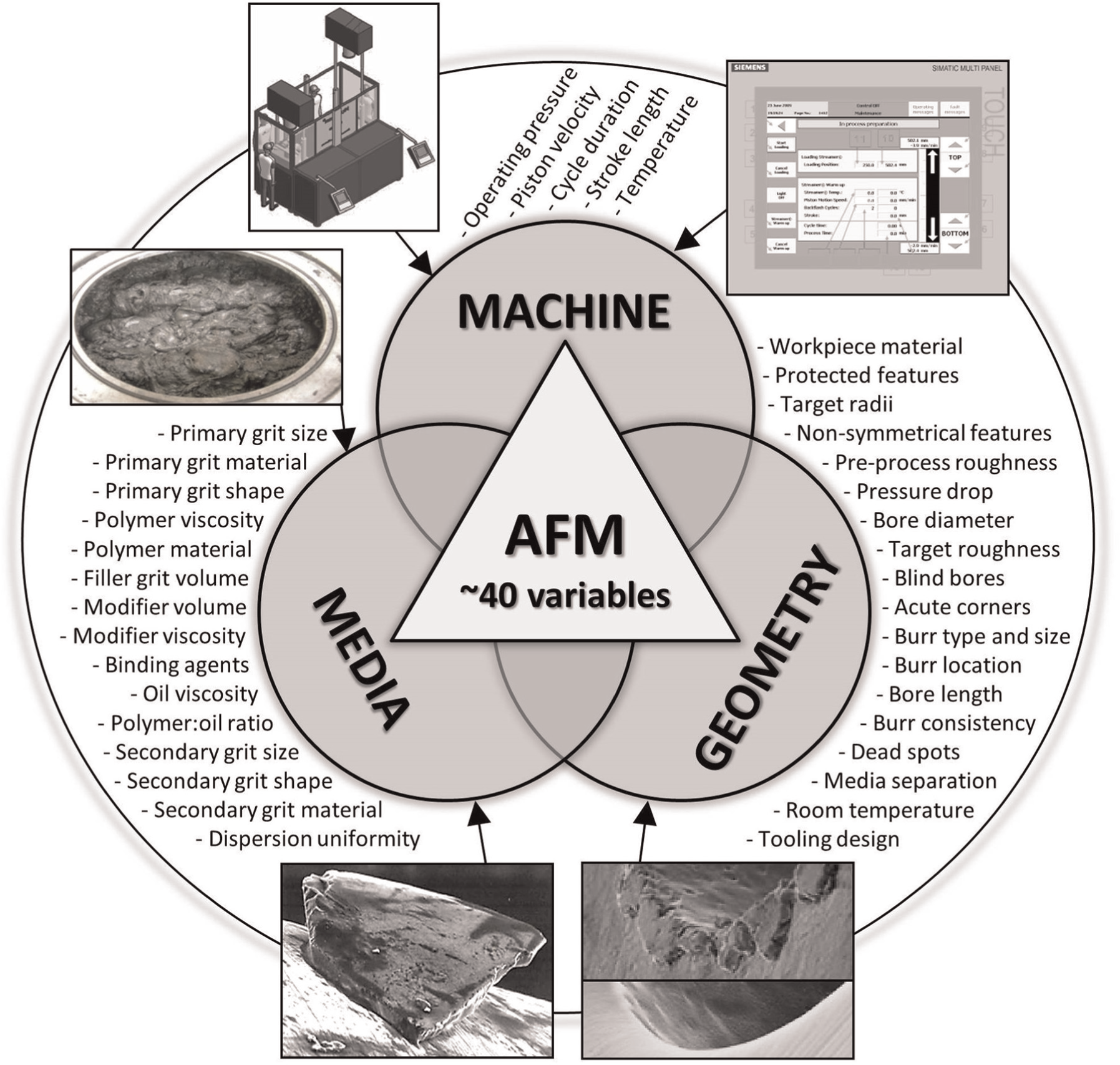
Identification of process variables and their intrinsic relationships in AFM.

Multivariate processes are often difficult to understand and characterise ⁶ – they can be rife with systematic error and results can be misleading to a user or researcher. AFM is typical of this type of system – a level change in any of the identified variables of Figure 1 can affect multiple other factors and void any accurate process prediction. In order to provide confidence in the process, we must combine variables into more manageable units, comprising multiple fixed levels. Combining variables and fixing others implies an intrinsic relationship between those joined factors, and consideration of the effects of joining two previously independent factors must be made.

In order to progress the AFM process and improve its accessibility to lay users, the issues associated with the multiple variables must be minimised. Main technical challenges include the following: (1) determination of effect on surface for a given combination of machine–media–geometry (MMG), (2) transferral of experimental results to an untested geometry and (3) catering to arbitrary part condition ⁷ (burr size, surface finish) as caused by (numerous) preceding operations. This study focuses on the machine corner of the ‘AFM triangle’, consisting of variables such as pressure, velocity, duration, length and temperature. These factors allow the user to manipulate the final result within the limitations of the geometry and media. Previous works^7,8–12 attempting to develop prediction models contain process factors from different corners of the AFM triangle, making it difficult to separate their findings and reapply them to other MMG combinations. Critically, the data collected in this research are to be reapplied as a benchmark in a computational fluid dynamics (CFD) simulation environment – while hand calculations and experience can often provide a user or researcher with an estimated process model, the geometry of the production components can vary in complexity – if a well-designed experiment can accurately interpolate missing values between and outside experimental levels, then we can be sure of the data quality and correlate experimental response values with simulated response values. This technique has not been previously applied and promises to lead to a full AFM simulation, providing value and viability in an industrial environment by removing costly trial-and-error steps in development of process models.

Common to all experimental investigations described above is the tendency to study groups of factors from different corners of the AFM triangle, which prevents us from isolating corners of the triangle in a simulation environment. Without knowing the effects of a complete set of machine (or media or geometry) factors, we are unable to verify experimental results against simulated results, and thus are liable to accredit changes in response variables to the incorrect factors.

Therefore, it is essential and much needed to undertake an integrated systematic investigation on the AFM process and thus develop an industrial-feasible scientific approach to render the process operating in a truly predictable, producible and highly productive manner. The research presented in this article attempts an integrated systematic investigation of the AFM system through investigating the collective effects of process variables on surface generation in AFM of titanium alloy 6Al4V.

CFD simulation-based analysis on the machine effects

As a scientific and viable production technique, readily available CFD software can be used to analyse the flow of media in an arbitrary geometry. While the rheological behaviour of the media will vary depending on its chemical makeup and grain fraction, there will always be the opportunity to determine its behaviour through simple assessment of viscosity versus shear rate, collected with a rheometer. What is unavailable, however, is the facility in software to simulate the size, shape, hardness, dispersion and general grit surface contact interaction model that the process desperately needs. Also unavailable, yet critical, is the processed length. The method presented here is the holistic embodiment of the CFD simulation-based approach as proposed by Howard and Cheng’s, ¹³ which is an effective and industrial-feasible‘workaround’, comprehensively integrated approach as illustrated in Figure 2.

Figure 2.

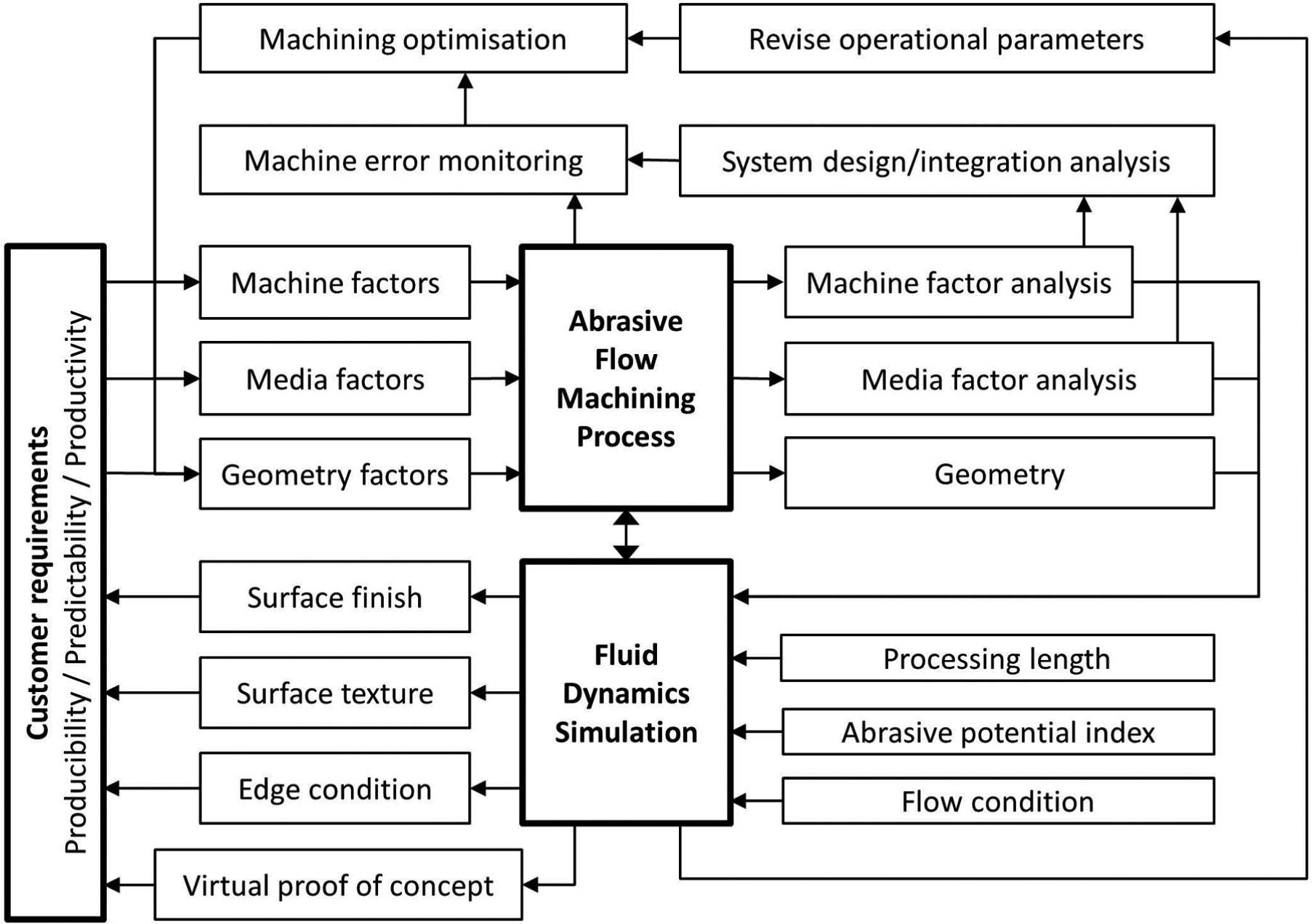
Map of CFD integration with AFM.

An accurate representation of flow condition at the point of interest (POI) (in the testpiece geometry) is simulated using CFD-based simulations and checked for sensible results against measured results (collected through experimentation in entire machine process space). We then re-employ the simulation in more complex geometry, checking the flow condition at the POI. The results remain valid, assuming we are using the same media – in turn, we also retain the ability to simulate with differing machine factor values; the simulation software will display a different flow condition, and therefore we predict a reasonable result based on testpiece results and extrapolations. Geometry can also be altered infinitely at this point.

The final consideration is the integration of the grit within the media and the workpiece material. This interaction requires the addition of values that are unable to be simulated – the three factors are length, workpiece material and the abrasive potential of the media (determined by its volume and size of grit) which is an as-yet unknown quantity pending further research.

Experimental set-up and validation

Defining process behaviour through experimental investigation of all factors in Figure 1 is needlessly complex and economically costly. Instead, we identify which variables may be condensed and revise our experimental factors and levels accordingly. In the case of this research, we are looking at pressure, velocity, temperature, stroke length and number of cycles.

Procedure, design of experiments and parameterisation

In order to isolate the effects of changing machine levels, we must fix the other two corners of the triangle – the control variables. The experiment uses a media supplied by Micro Technica^® Technologies GmbH, MF10-24B(60)-40B(60)-400B(40) – the naming convention of which implies an unknown (approximately 100 Pa/s) polydimethylsiloxane (PDMS) carrier and three grit sizes of Federation of European Producers of Abrasives (FEPA) mesh sizes F24, F40 and F400 (710, 425 and 17 µm). Weighting is 35% grain fraction − 65% carrier. Within the grit, there is 25% by weight of F400 as filler grit, while the larger (75%) particles provide the MR ability the media is designed to achieve.

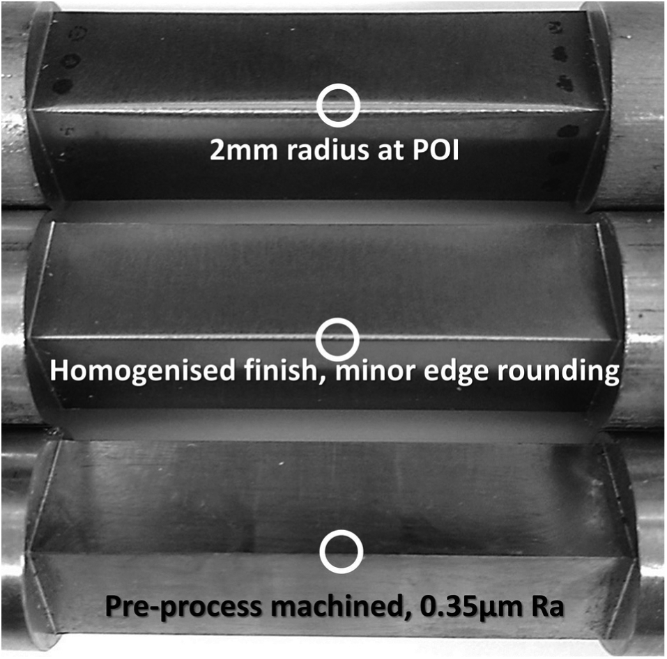
We also control our geometry as shown in Figure 3; the media is funnelled through a series of reducing rings into the main testpiece support. This is a 40-mm tube formed of a steel body and replaceable nylon liner, with a bore crossing through halfway allowing the insertion and orientation of the testpiece. Non-Newtonian media flow through the tube causes the media at the outer walls to travel at reduced velocity, hence the wear pattern in the upper sample in Figure 4. Data are only collected from the centre line, to be assured that the user-set velocity is in full effect.

Figure 3.

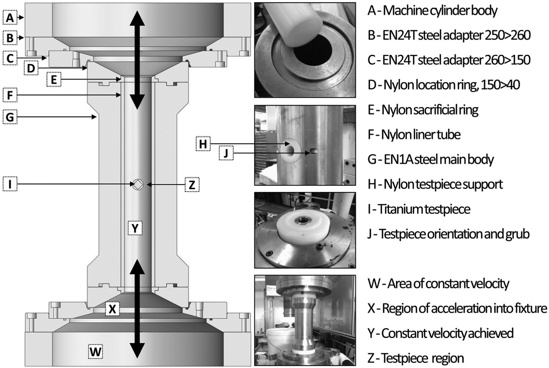
Experimental set-up in section view.

Figure 4.

Titanium testpiece form; all samples contain a centre section of 10 × 10 × 40 mm.

Variables are reduced from five to three; the stroke rate and number of cycles are compounded into a derived unit of quantity of processing (m), whereas pressure is discounted as the machinery requires a user-set velocity – pressure is delivered to reach the required level. Experimental factors are therefore set to velocity, temperature and quantity.

Prior works have shown a three-level experimental strategy to be a wise choice^10,12,14 as effects are known to be nonlinear. The minimum 3³ requirement allows the use of response surface methodology (in the form of the Box–Behnken design), known for ease of modelling quadratic functions, functioning most reliably when levels are moderate (representative of practical process values) and greater efficiency than the Central Composite Design (CCD) when studying under four factors. Table 1 shows the selected process factors and levels.

Table 1.

Process factors and levels’ selection.

Factors	Levels	Derived	M/C value
Velocity	+1	325 mm/s	280 mm/min
	0	230 mm/s	195 mm/min
	−1	100 mm/s	85 mm/min
Temperature	+1	45°	45°
	0	35°	35°
	−1	25°	25°
Quantity	+1	250 m	Stroke 150 mm, cycles 42
	0	145 m	Stroke 146 mm, cycles 25
	−1	40 m	Stroke 144 mm, cycles 7

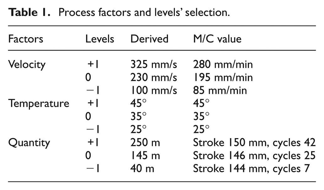
The structure collects 12 datapoints from the edges of the process space and multiple centre points. The researchers deemed it necessary to include off-line repetitions before integrating values of higher accuracy into the process model. Level’s selection was achieved by determining the least (V−, T+) and most (V+, T−) demanding to pump by trial and error. The Hagen–Poiseuille equation was used initially to help design fixture geometry using media viscosity calculated through machine back-pressure requirements – the equation only applies to laminar flow and we have exceptionally stable laminar flow of Re = 0.043.

Velocity drives the delivery of the media – we are limited to 300 mm/min (0.005 m/s) in terms of machine maximum capability; an upper level was set at 280 mm/min (0.0046 m/s) after testing with the lower level for temperature. Our fixture geometry combined with media viscosity drives a linear acceleration based on cross-sectional area (CSA) whereby the piston diameter of  ∅250 mm (CSA 0.049 m²) can be compared to the two ‘half-rounds’ left by the flow passage on either side of the workpiece edge of CSA (0.000696 m²), creating a ratio of 1:70 between machine and workpiece POI. Our upper level of 0.0046 m/s is now known to be travelling at 0.322 m/s at the POI. This extends to levels 0 and −1.

Media temperature is controlled by a closed-loop system whereby a probe constantly monitors for changes, activating a refrigeration loop or deactivating to allow the permanently installed and functioning heating mats to raise the temperature. Through experience, media is known to undergo viscous heating, where operation at high pressures causes internal friction between shear planes to heat beyond the capacity of the refrigeration system. The occurrence is minimised by operating the machine within tolerable limits.

Similar to velocity, we must retain transferability in quantity, that is, our input levels must be related to the POI. Since the volume of media in the machine cylinder (0.00736 m³ (150 mm stroke)) is greater than the volume in the fixture (0.000373 m³), we can establish that the ratio of volume is 1:19.73. Therefore, cylinder travel drives media contact with the sample surface by this ratio, equating to a −1 level of 150 mm stroke (1 cycle = 2 strokes) at seven cycles (total of 2 m machine travel). A total of 2 m of machine travel is equal to ∼40 m of processing within all surfaces in the fixture. The testpiece is processed with 40, 145 and 250 m.

Analysis of effects on surface features and process capability

Responses are recorded for three dependent variables: average surface roughness (Ra, µm), MR (mm²) and peak height reduction (PHR, mm). These units are selected based on industrial requirements for geometry specification. Surface roughness is typically a ‘no-more-than’ specification, so improvement upon customer values (or preprocess experimentally derived predictions) is acceptable. In the case of MR and PHR, edge rounding requirements in customer specifications typically specify a tangential radius between two other features where the radius value is toleranced by a range throughout which it may fall ‘non-tangentially’.

Radii tolerances are based on feature function; Mollart Engineering Ltd frequently deals with components where intersecting features are responsible for carrying wires or hydraulic fluids. These functions require features that are simply rounded to an extent that insulation may not strip from wire, or that flashing and debris may not enter a stream of hydraulic fluid. MR as a response is implemented in this research for the purpose of comparing a simulated flow regime to physical MR – we evaluate the X–Y plane of the testpiece at the point of greatest velocity for greatest accuracy. PHR is an unconventional unit derived in this research for the purpose of differentiating between area reduction (catered for by MR) where the MR value may not describe the erosion of a peak – that is, MR has occurred, but the location of MR (while still high) has left a functionally undesirable edge. PHR describes the erosion level perpendicular to the flow path.

Measurement of these responses is achieved with two instruments; roughness is measured with a non-contact solution – a white light interferometer (WLI) (ZYGO NewView^™ 5000). MR and PHR are measured with a Mitutoyo’s CV3100 Formtracer series.

Figure 5 illustrates the mind-mapping process of collecting data from the component samples, conversions and resultant numerical outputs by using preprocess engineering analysis, shop-floor metrological measurement and post-process data processing and result’s formulation.

Figure 5.

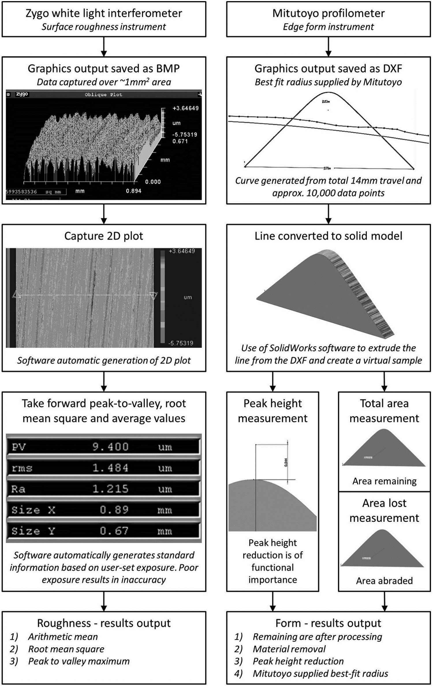
Process of collecting data from samples, conversions and resultant numerical outputs.

Average surface roughness (Ra)

Samples started with a consistent 0.35 µm surface roughness milled finish, resembling a reflective polished finish. Grey, non-reflective finishes were seen on all processed components, even those with improved surface finish – this points to a ploughing mode of MR, whereby the sheared surface of a milled finish promotes a mirror finish and AFM shows a dull finish (with this grit size) based on the random dispersion, size and orientation of the grains. Finish was, however, homogenous – having removed any sign of milling tool path, which has key importance in applications of cosmetic value.

Average roughness responses are collected in the range 0.239 and 1.252 µm, while standard deviation (SD) between repetitions is<0.08 µm. Datapoints have been plotted in a run order versus response scatterplot, whereby results are spread throughout the process space, showing a low likelihood of machine bias. Figure 6 displays three WLI images, from roughest to smoothest – despite the application of F24 grit (mean size 686 µm), we are able to alter the surface condition within this range, in this geometry condition. The far left interaction plot shows that (with average quantity) roughness will linearly increase with velocity when processed at 35 °C. Velocity has little to no effect on surface roughness when operating beneath ∼200 mm/s at extreme ends of the temperature scale – this can be explained by matrix and reinforcement principles; at low temperature, the matrix is stiffer, preventing free grit orientation and thus improving the shearing mode of MR – the carrier’s dilatant (shear thickening) behaviour increases under increased velocity. The centre interaction plot is useful for an operator; it shows increased quantity of processing to steadily increase roughness, irrespective of velocity. The Q = 250 m line shows a tapering off, indicating an effect similar to that of using different grades of sandpaper – eventually, the grain size in media will reach a terminal roughness value, where neither quantity, temperature nor velocity had any impact. The right-hand plot shows how temperature dominates as a single factor – consisting of 30% of total effect on the surface, increasing temperature results in improved surface finish – contrary to the left plot, we may simply be placing the grits into different modes of MR; for the same grit size, a stiff matrix will provide an optically reflective surface through shearing, while a weak matrix will provide a non-reflective surface through ploughing. Both surface finishes will be the same. Temperature, velocity–temperature interaction and quantity are found to be the three most significant terms (in that order) in ability to affect surface roughness.

Figure 6.

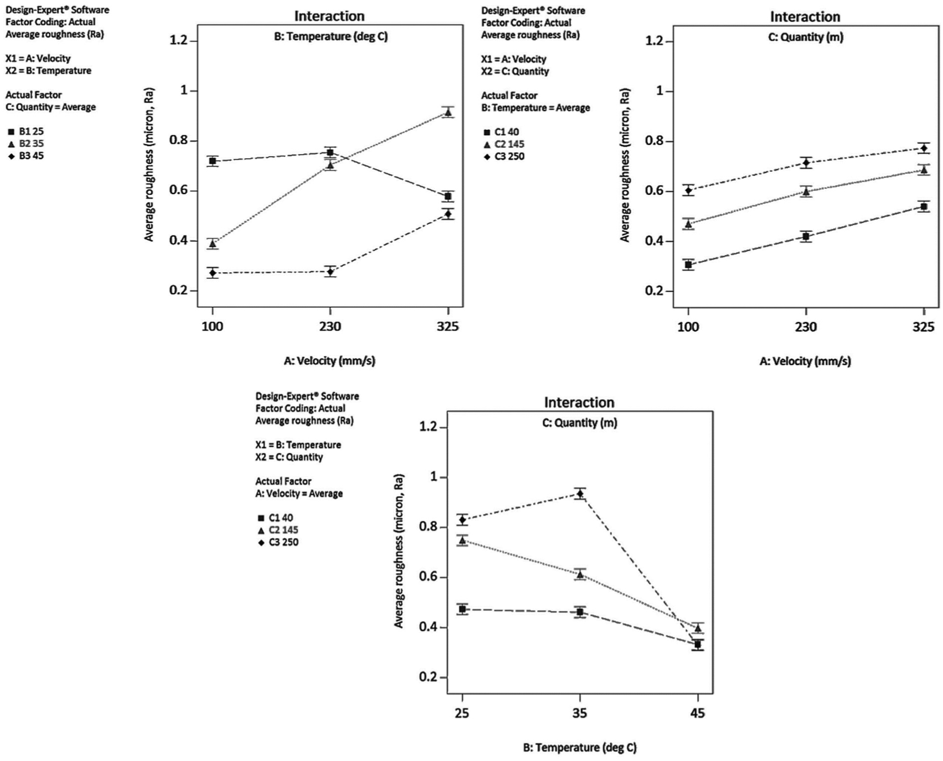
Three plots from a WLI and three interaction plots between velocity, temperature and quantity.

Material removal (MR)

Starting with a 90° edge positioned at 45° to the flow field, edge geometry is consistent between all samples, where error is limited to the milling machine rotary table accuracy of 5 arc-seconds, used to position the four faces of the square section. Using the Formtracer instrument output, we know that radii (where tangentially formed) range from 0.04 to 1.2 mm. Visually, it can be seen that edge rounding is not consistent along the sample length (see Figure 4), showing evidence of the non-Newtonian flow field in effect. We know that the machine’s greatest influence is exerted upon the centre line of the flow field, which dictates the measurement location.

Experimental levels have provided a range of values, from 0.07 to 1.03 mm²– SD between repetitions is <0.059 mm². An increased magnitude of variation was found when processing parts for longer duration and greater velocity, while empirical evidence suggests the machinery fails to retain standards of repeatability when the machine is forced to work harder and longer.

Figure 7 shows three plots of interaction: VT, VQ and TQ. Lower left considers a constant quantity of media and shows that with increasing velocity, temperature drives MR, increasing with velocity, apart from one exception at 25 °C where MR initially increases then reduces – increased viscosity at lower temperature provides greater support for abrasive grit, although if the media travels too quickly, edge conformity is reduced and MR is limited. This is reinforced by considering the same VT plot in Figure 8. The half-normal plot shows that VT is responsible for 20% of total MR effect. The centre VQ plot shows that rate of change of MR increases linearly with velocity, but quantity increases roughness by 0.2 µm for every 100 m of travel. Naturally, these values are only relevant to this media and geometry, but the effect would scale accordingly elsewhere. The right-hand interaction is between temperature and quantity; TQ is responsible for over 37% of total MR effect and shows that a higher quantity of processing will remove more material, but combined with temperature change of ∼20 °C, we can more than double the effect. Approaching 45 °C, MR is poor irrespective of processing quantity. Irregularity between line gradients at different processing quantities suggests another physical phenomenon is manifested, as we expect the gradients to travel in a similar direction when treated with scaling variables. In this instance, we are likely seeing the effect of media viscosity and edge conformity.

Figure 7.

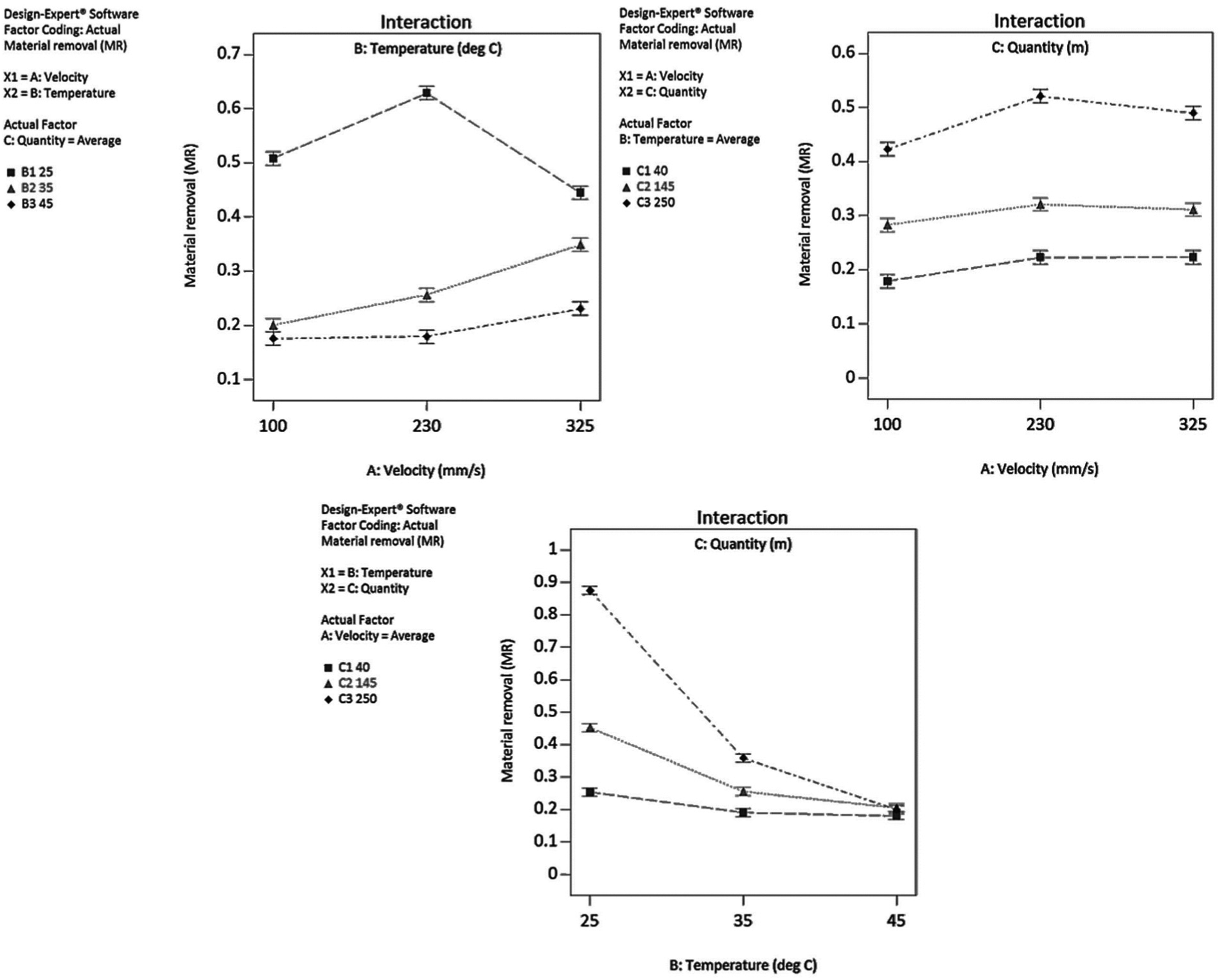
Three plots derived from Formtracer output and three interaction plots.

Figure 8.

Three plots derived from Formtracer, solid modeller output and three interaction plots.

Peak height reduction (PHR)

Dimensions of the sample in processing orientation are known, where the preprocess peak condition can be overlaid on the Formtracer output – this allows a single numerical value to be measured between the previous and current peak height, which differentiates itself from MR by referring specifically to the reduction of the functionally important edge. The measurement is collected normal to the flow field, from the same data as the MR output, and therefore only in the centre of the flow field.

In contrast to the other responses, PHR offers the greatest spread of points across the process space and a maximum SD of 0.057 mm. A similar phenomenon is noted as with MR – deviation between repetitions is greater in trials of high velocity and quantity. Error is well distributed about mean values, as evidenced by bars in Figure 8.

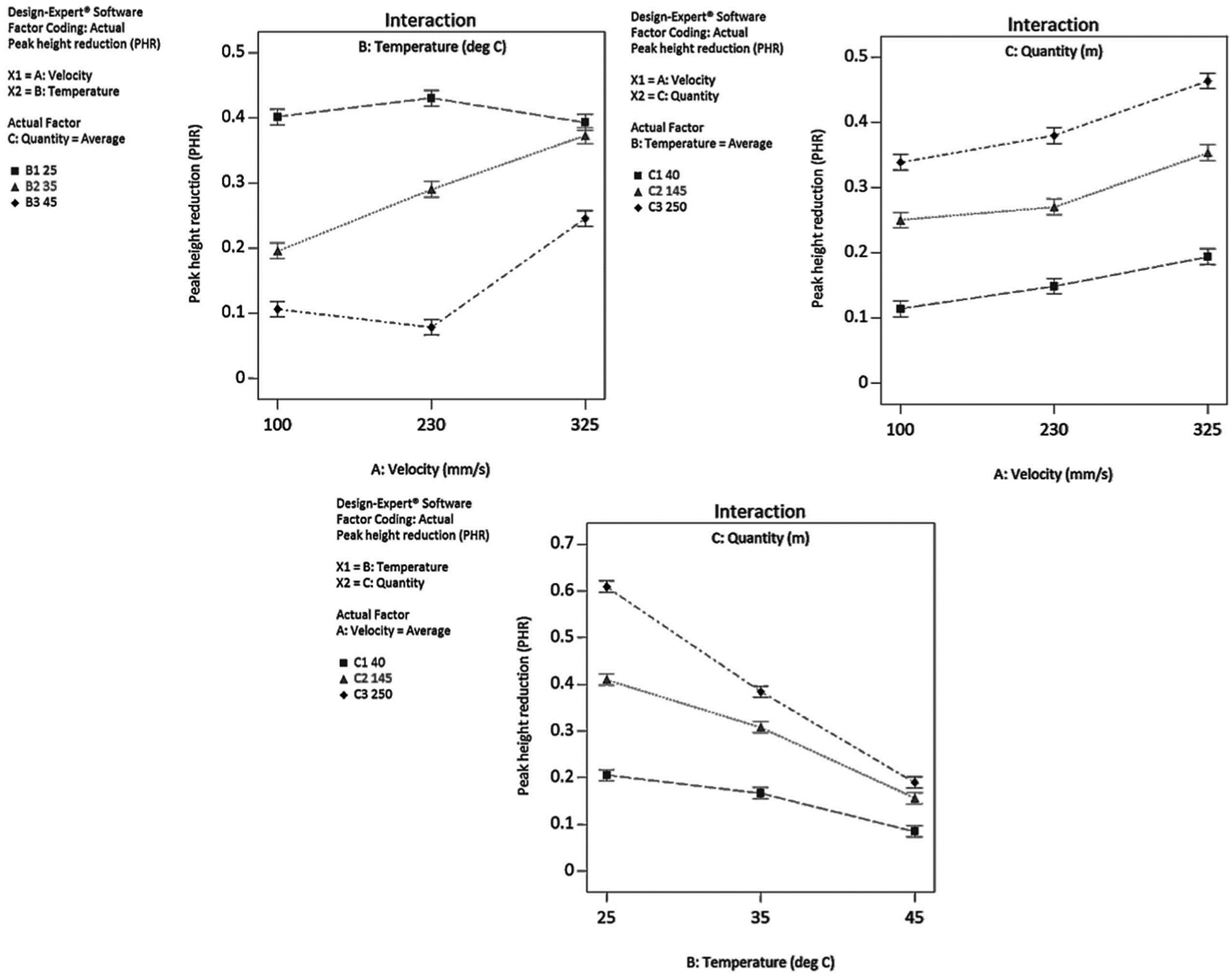
This dataset offers a range of responses from 0.05 to 0.667 mm, allowing a significant degree of control over the edges in production parts, equating to a 1.5 mm radius. The interaction plots in Figure 8 highlight the differences in PHR to MR; PHR is driven by quantity. A total of 35% of PHR effect can be attributed to this factor. Second, the temperature–quantity interaction makes up the next 18% of the effect.

The leftmost interaction plot in Figure 8 shows that increasing velocity will generally increase PHR, and response magnitude is strongest at higher temperature, likely due to increased shear thickening behaviour under increased pressure. Looking closer at 25 °C and 35 °C highlights the same viscosity to geometry-conformity flow problem, where at 35 °C a linear improvement in PHR is achieved, but a negative response at 25 °C questions previous assumptions of ‘the more viscous the media, the greater the edge rounding’. Given geometrical complexities in production parts, this is a significant finding, as it can be argued that an optimum flow field condition is necessary, one which is controlled by velocity and temperature.

The centre interaction plot identifies quantity to be insignificant to process outcome when manipulated with velocity – PHR levels are offset by varied quantity by a uniform 0.1 mm PHR/100 m quantity. Increasing velocity has no effect on gradient of response. This is useful in a production environment when a user needs to predictably gear up or gear down a response value.

The leftmost plot shows the TQ interaction, whereby PHR levels are significantly altered when low temperatures are combined with high quantities. Processing quantity can be limited by high temperatures, much as with MR; at 25 °C, 0.2 mm PHR is achieved per 100 m processing; however, that value reduces to 0.1 mm PHR per 100 m processing at 35 °C and ∼0.03 mm per 100 m at 45 °C.

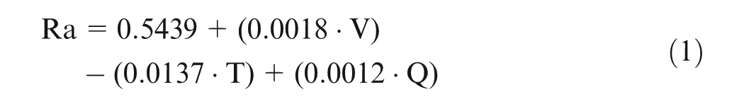
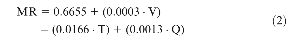
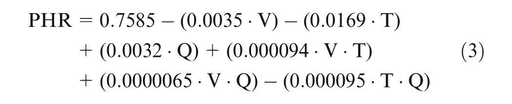
Predictive model

Data collection activities have provided the ability to produce type III analysis of variance (ANOVA) tables, which are re-employed with software to create predictive equations based on data best fit estimates – each of the three responses from a 3³ full factorial design is converted into datapoints required for the response surface methodology (RSM) Box–Behnken design. Surface roughness and MR data are calculated to fit best to a linear model, while PHR fits a two-factor interaction (2FI) model

$$\begin{array}{c}\multicolumn{1}{c}{\text{Ra}=0.5439+(0.0018·\text{V})}\\ -(0.0137·\text{T})+(0.0012·\text{Q})\hfill \end{array}$$

(1)

$$\begin{array}{c}\multicolumn{1}{c}{\text{MR}=0.6655+(0.0003·\text{V})}\\ -(0.0166·\text{T})+(0.0013·\text{Q})\hfill \end{array}$$

(2)

$$\begin{array}{c}\text{PHR}=0.7585-(0.0035·\text{V})-(0.0169·\text{T})\hfill \\ +(0.0032·\text{Q})+(0.000094·\text{V}·\text{T})\hfill \\ +(0.0000065·\text{V}·\text{Q})-(0.000095·\text{T}·\text{Q})\hfill \end{array}$$

(3)

Naturally, these findings are only applicable to this combination of media and geometry, but critically the results are able to extend the findings of the study for the purposes of dataset extrapolation – increasing the verification possibilities where simulation of results is concerned (within limits of model error). Figure 9 displays the results of model application by plotting values of the collected datapoints with respect to the model’s predicted positions – additional verification points were sourced by adopting the missing experimental configurations of the Box–Behnken from the 3³ factorial design. Figure 9 also contains verification points, that is, points captured at arbitrary locations within the process space – these are marked on the plots; there are three unique combinations, plotted on each of the three response variable plots.

Figure 9.

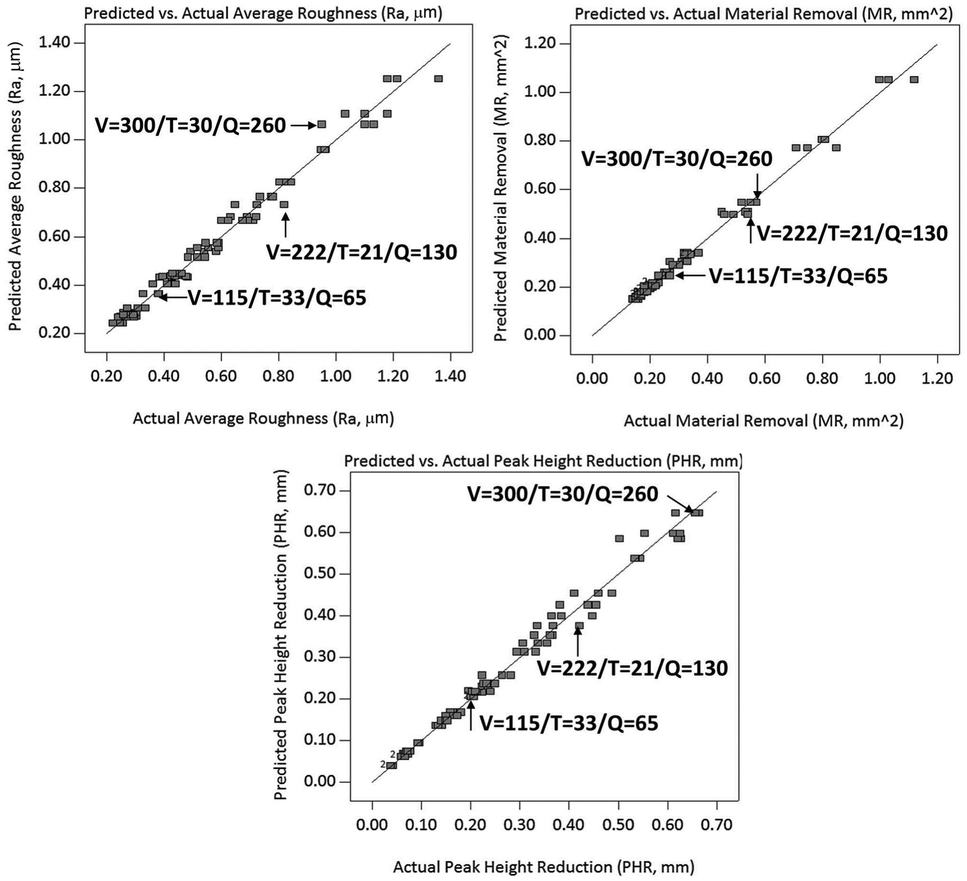
Plots of best fit for actual values against predicted values for responses.

An industrial case study on an oil and gas industry component

An industrial case study is carried out by immediate transferral of the AFM approach and its industrial implementation perspectives to AFM processing of a complex oil and gas industrial exploration component. The findings discussed in section ‘Analysis of effects on surface features and process capability’ can be considered relevant when considering the POI in the component contains a 90° edge where flow travels at 45°, a velocity over the POI is calculable using a CSA conversion and processing volume is converted by dividing volumes. Figure 10 shows the results of 325 mm/s, 35 °C and 370 m of AFM processing of the component as required by the industrial company. Empirical evidence and prior research ¹⁵ suggest that a VQ interaction controls the differential in edge rounding between the radii of the slots and the long side – quantity discrepancies occur between the centre of the slot and the edge where a less restrictive path is found through the centre. Excessive velocity prevents the top edge of the slot from obtaining sufficient processing due to geometry-determined flow path – this can be improved by reducing velocity to allow a more uniform distribution of pressure around the inside of the port. Visualisation of this effect will be presented in further work.

Figure 10.

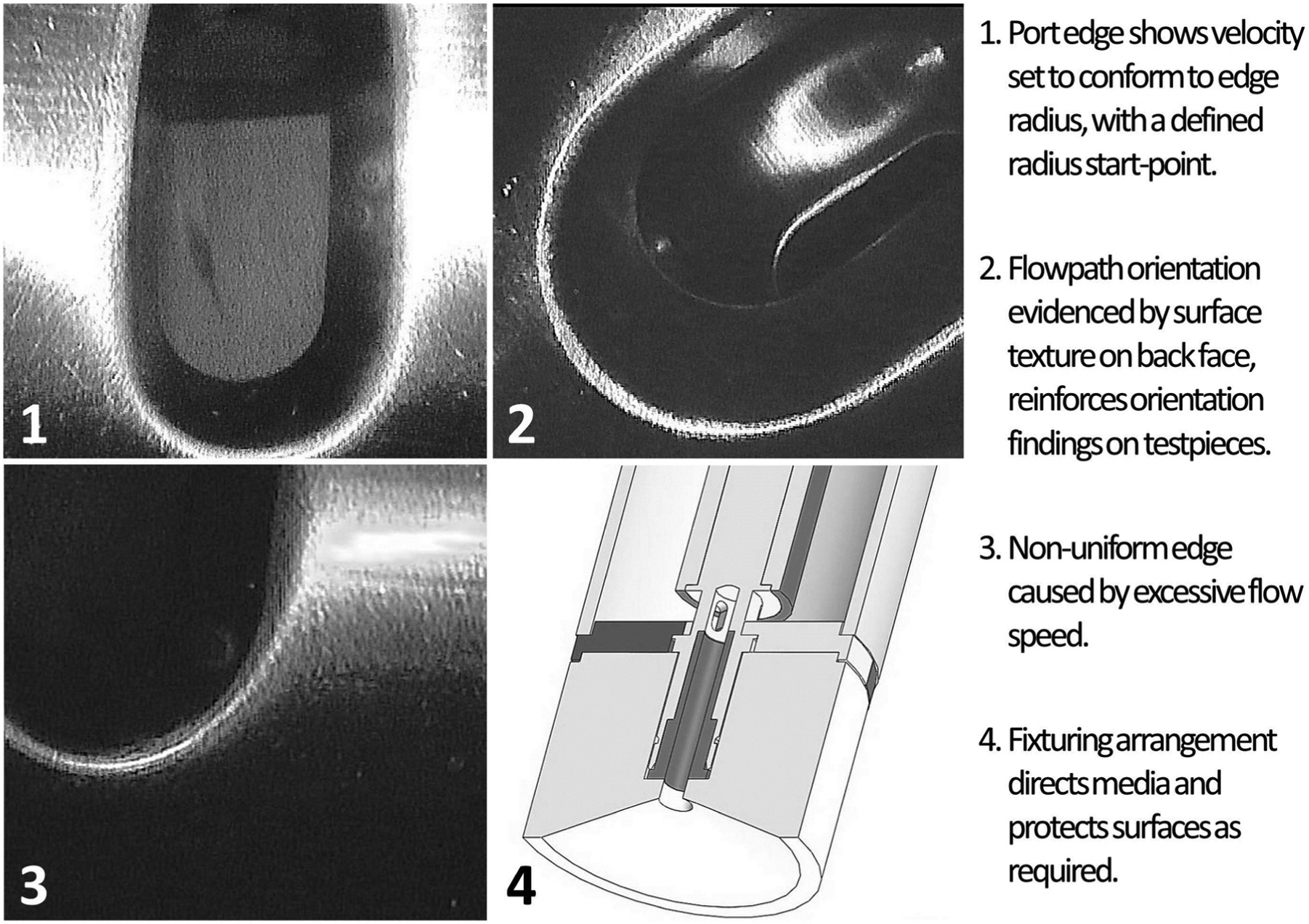
Areas of component inspected with ∅4 mm CCD camera on articulated head.

Future applications of the process include surface finishing of medical-grade titanium alloy implants, produced by ALM, specifically through the direct metal laser sintering (DMLS) process. Comparatively, the material is more ductile and fracture-resistant than common grade 5 for bone-contact applications, which theoretically demands more from the AFM process. These materials are able to be produced in the geometry used in the testpiece environment of the study presented in this article – by adopting the same test methodology, erosion achieved is known, test shear conditions are known (as the simulation does not alter) and correlation between input and output is derived – in little more than 13 samples (minimally populated Box–Behnken RSM design), it is possible to characterise AFM’s capability with a new material. To enhance the level of control, an experiment has been completed to deliver equivalent data from a 3³ RSM design studying carrier viscosity, concentration of abrasive and grit size.

Conclusion

In this article, an integrated systematic investigation is presented by focusing on the collective effects of the process variables on surface generation in AFM of titanium alloy 6Al4V. The integrated systematic approach aims to render the AFM process in a predictable, producible and highly productive scientific manner. The key variables in the machine corner of the AFM triangle are identified and studied. Each of the response variables studied scales in relative proportion with one another, proving that increased MR and PHR will result in poorer surface roughness values, for a constant media and geometry. The following conclusions are further drawn up:

• Optically non-reflective surfaces will be common in edge rounding operations without consideration to a secondary ‘fine grit’ stage to mimic the lapping process.

• The process is useful for cosmetic purposes to eradicate a mixture of machined surface finishes by ‘overwriting’ the finish with its own.

• For the majority of samples, roughness results exceeded the preprocess condition, calling into question the applicability of AFM for surface finishing – grit sizes and grain fractions will be studied in consequent work as prior literature shows improvements with finer mesh grit.

• Edge rounding of titanium alloy 6Al4V with media of primary grit size ∼700 µm can be achieved up to ∼1.5 mm, dependent upon carrier behaviour.

• Material is removed through the mechanism of ploughing and rubbing in the direction of flow as shown by the WLI images.

• Feature alteration is driven by temperature and quantity. These factors are therefore considered more critical for a production environment.

• Temperature drives surface finish in this experiment, and we know the response of viscosity to temperature to be linear, reducing with increased heat – the interaction of viscosity and grit size is therefore important to understand clearly in future work.

Furthermore, considering the importance of temperature to all responses variables, it must be concluded that rheological state of the carrier is of significant influence to process outcome. Two further research interests are identified with industrial significance, that is, a study of media factors, isolated in the media corner (as in this experiment) and a study to correlate response variable values with a simulated value to prove viscosity-edge conformance assumptions.