Adaptive simulations in T-shape tube hydroforming with different outlet diameters

Abstract

A successful tube hydroforming process depends largely on the loading paths for controlling the relationship between the internal pressure, axial feeding and the counter punch. The objective of this article is to propose an adaptive control algorithm to determine appropriate loading paths in T-shaped protrusion hydroforming with different outlet diameters. The finite element analysis is used to simulate the flow pattern of the tube during tube hydroforming process. The analytical flow line net configuration of the tube is utilized to determine the speed ratio of the counter punch to the axial feeding at the protrusion stage. Appropriate loading paths for different outlet diameters are determined using the proposed adaptive control algorithm. Different pressurization profiles are used in the tube hydroforming experiments. Experimental results show that a sound product is obtained using the pressurization profile determined by the proposed adaptive simulation algorithm. From the comparisons of the product shape and flow line net configurations between the analytical and experimental values, the validity of the proposed control algorithms is verified.

Introduction

Tubes with different diameters in their outlets are widely applied to pipe fitting, automobiles, bicycles, and shipbuilding industries. Tube hydroforming (THF) is an innovative manufacturing process widely applied to manufacturing tubular parts in various fields due to the increasing demands for lightweight parts. ^1,2

If the pressure and axial feeding are not appropriately applied to the hydroforming process, wrinkling at the guiding zone and bursting or overthinning at the branch part will probably occur. A few studies have been published to discuss the loading paths for obtaining a better profile and thickness distribution of the formed product. For example, Jain et al. ³ used LS-DYNA to simulate a dual hydroforming process and discussed the effects of counter pressure upon excessive thinning and premature wrinkling. However, the linear loading path was obtained by trial and error. Strano et al. ⁴ proposed a geometrical wrinkle indicator to evaluate the occurrence of wrinkle and used the finite element (FE) software to simulate THF processes. Aue-U-Lan et al. ⁵ used the maximum thinning as a fracture criterion during their adaptive simulations of loading paths. Ray and MacDonald ⁶ proposed a fuzzy control algorithm combined with FE simulations to determine the optimal loading paths for THF process. Manabe et al. ⁷ used the fuzzy theorem to obtain an adequate loading path for T-shaped hydroforming processes. Ngaile and Yang ^8,9 have published a series of studies involving analytical models for the characterization of various tube-shaped tribotests in THF processes. Hwang and Lin ¹⁰ presented a FE model to simulate the T-shaped hydroforming processes with internal pressure and axial feeding. The friction coefficients between the tube and die for different lubricants were also discussed. ¹¹

Weight reduction is an important issue. Applications of the THF technique and magnesium alloys offer feasible approaches for lightweight products in various areas. However, due to the hexagonal close-packed structure, magnesium alloys exhibit poor formability at room temperature. As a result, magnesium alloy parts are usually manufactured at elevated temperatures. Neugebauer et al. ¹² developed a warm hydroforming machine for T-shaped tubes and carried out experiments of magnesium alloy tubes. Okamoto et al. ¹³ discussed the optimal conditions of metal mold shape and the effects of surface roughness on process formability during T-shaped protrusion of magnesium alloy tubes at elevated temperatures.

Lorenzo et al. ¹⁴ implemented an artificial intelligence system based on fuzzy logic for THF process design to achieve a defect-free and desired final shape of the component. Mohammadi et al. ¹⁵ proposed an optimization approach for the loading path of THF of an aluminum T joint with the finite element method (FEM) using a commercial code. The objective function is the clamping force, and the constraints of wrinkling, minimum thickness, and calibration should be achieved. The objective and constraint functions are obtained by training a neural network and the objective function is minimized using several optimization methods including hill-climbing search, simulated annealing, and complex method. Seyedkashi et al. ¹⁶ developed an optimization method for the warm THF process using the simulated annealing algorithm with a novel adaptive annealing schedule. The optimal pressure loading paths are obtained for AA6061 aluminum alloy tubes with different wall thicknesses and corner fillets. Ngaile and Welch ¹⁷ presented a methodology of decomposing the pressure–displacement loading path as a time variable to obtain pressure–time and displacement–time variants that are optimal for the THF machine system. The THF experiments for double T-shaped parts are carried out to demonstrate that using different pressure–time and displacement–time variants can result in a significant increase in the maximum power required by the THF machine actuators.

So far, process loading paths during T-shaped hydroforming with different outlet diameters have not been discussed thoroughly in the literature. The present authors have developed a bulge test apparatus for bulge forming of magnesium tubes at elevated temperatures. ¹⁸ In this article, an adaptive simulation algorithm in T-shaped protrusion hydroforming with different outlet diameters is proposed. Loading paths for T-shaped hydroforming with different outlet diameters are determined using the proposed control algorithm.

Analytical model

Forming parameters

A tube with an initial length L₀ and an outer diameter D₀ can be compressed by two axial punches at its two ends and pressurized inside the tube simultaneously to form a T-shaped product with a branch diameter D_p. A schematic diagram of the T-shaped hydroforming process with different outlet diameters is shown in Figure 1. The left and right half portions illustrate the geometric configurations of the die and tube before and after hydroforming, respectively. The surface at the die fillet can be designed as an elliptical curve with axes R_a and R_b. The internal hydraulic media is input through an entrance hole to generate a high pressure P_i to bulge the tube simultaneously with the action of two pushing punches. A counter punch (CP) moving backward is applied at the late stage of the forming process.

Figure 1.

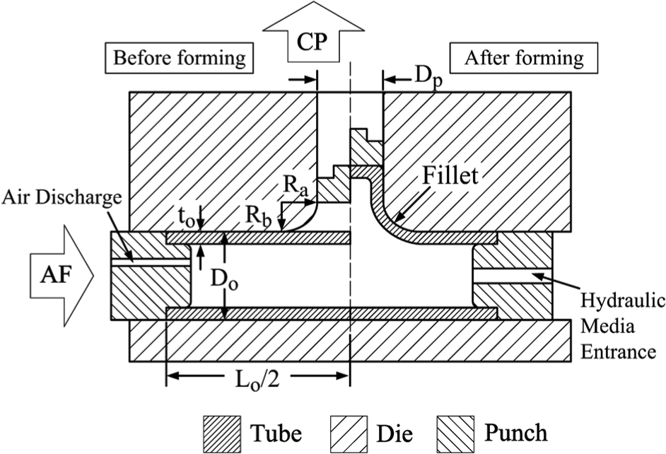
Schematic representation of a T-shaped hydroforming process with different outlet diameters.

A die shape called “pentagon die” is designed as shown in Figure 2, in which one quarter of the die surface at the transition zone is enclosed by five curves or straight lines, where B₁ and B₃ are two circular arcs on the surface of the branch and tube parts, respectively; B₂ is an arc along the die fillet; B₄ is a straight line at the tube side wall; and B₅ is a smooth curve that has zero gradients on the symmetric plane at the two end points. A Bezier curve with a third-order equation and four control points is adopted in this article. For the details, please refer to the study by Hwang et al. ¹⁹

Figure 2.

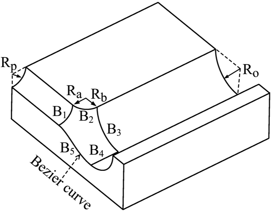
Schematic representation of geometrical configuration for a pentagon die.

FE simulations

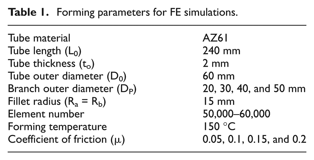
At first, the geometries of the objects were constructed using a commercial software SolidWorks. Then, a FE code DEFORM 3D was used to implement the simulation of T-shaped hydroforming processes. The die, axial feeding, and CP were regarded as rigid bodies and the tube was regarded as rigid plastic. The flow stresses of magnesium alloy AZ61 tubes for different temperatures and different strain rates obtained by compression tests are shown in Figure 3. The tube was divided into about 50,000 tetrahedron elements. There are four layers of elements in the thickness direction and the shape of the die is not so complicated; thus, reliable simulation results are obtained and justified by comparisons with experimental results. Other forming parameters are given in Table 1.

Figure 3.

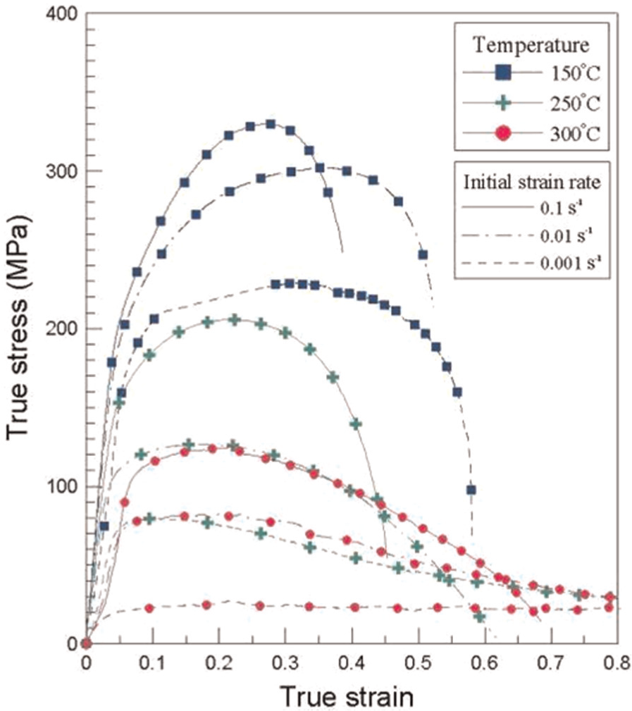
Flow stresses of magnesium alloy AZ61.

Table 1.

Forming parameters for FE simulations.

Tube material	AZ61
Tube length (L0)	240 mm
Tube thickness (to)	2 mm
Tube outer diameter (D0)	60 mm
Branch outer diameter (DP)	20, 30, 40, and 50 mm
Fillet radius (Ra = Rb)	15 mm
Element number	50,000–60,000
Forming temperature	150 °C
Coefficient of friction (µ)	0.05, 0.1, 0.15, and 0.2

Adaptive control algorithm

The forming process is divided into two phases: bulge stage and branch protrusion stage. At the bulge stage, the internal pressure is increased and the axial feeding is moved forward. But, the CP is kept still. An initial pressure of P_i = 4σ_yt_o/(D₀ − t_o is set. At the early bulge stage, the internal pressure is continuously changed according to an equation of P_i = 2σ_yt_o/R, where R is the radius of the free bulge region inside the branch cavity. A flow chart for the bulge stage during T-shaped protrusion forming is shown in Figure 4. At first, the parameters, such as the material properties, die geometry, internal pressure increment (ΔP_i), and axial feeding increment (ΔF_a,), are input. At the early bulge stage, as shown in Figure 5(a), the thickness ratio t/t_o at the top position P is checked. If it is smaller than 90%, the internal pressure is decreased, the axial feeding moves forward by one step, and then the simulation procedure is repeated. After P is in contact with the CP, the process proceeds to the late bulge stage, as shown in Figure 5(b), and separation at the die fillet and wrinkling at the guiding zone are checked. If the result is yes, the internal pressure is increased, the axial feeding moves forward by one step, and then the simulation procedure is repeated. After the contact length ratio L_cp/D_p reaches 80%, the simulation goes to the branch protrusion stage.

Figure 4.

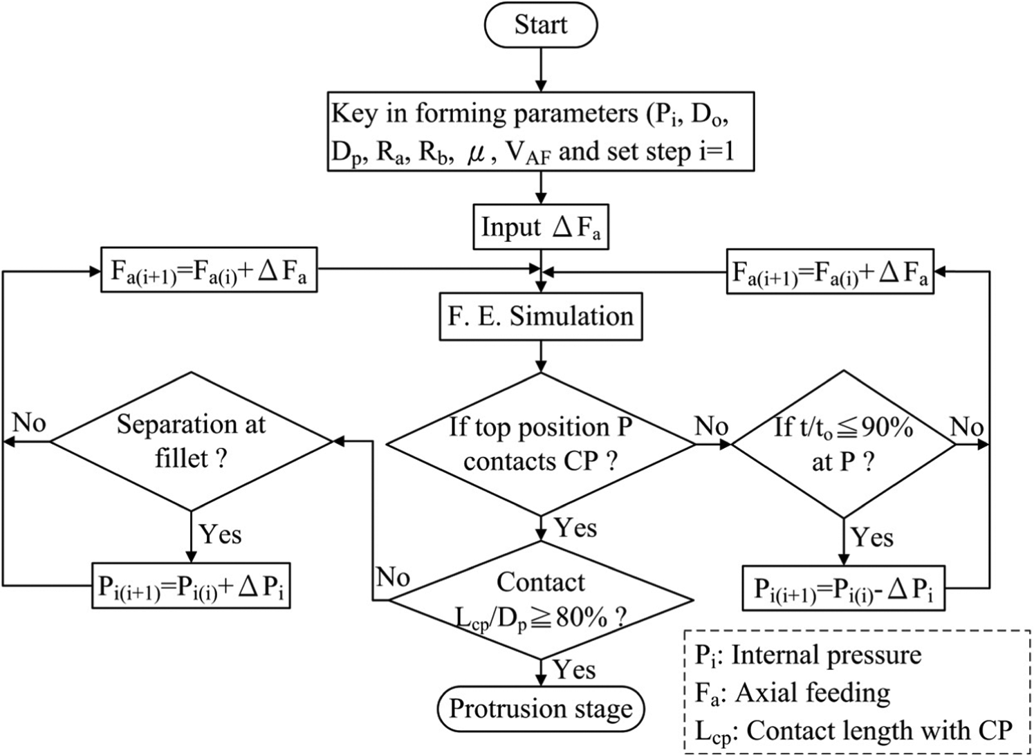
Flow chart for adaptive simulation at bulge stage of T-shaped hydroforming.

Figure 5.

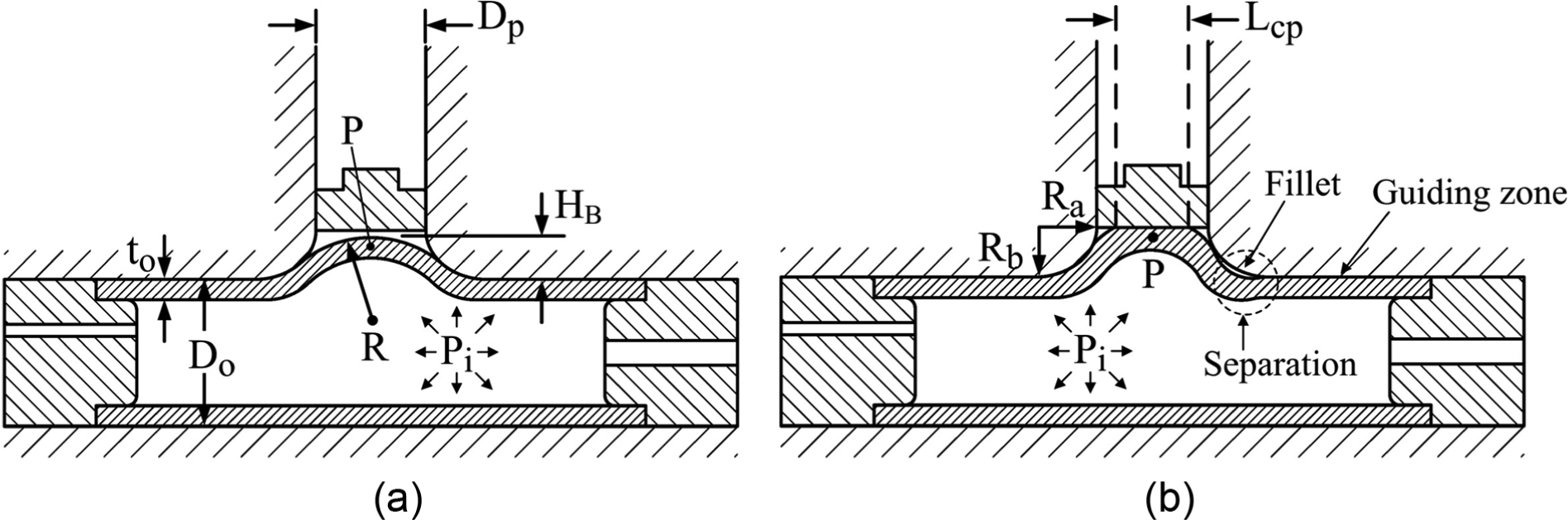
Schematic representation of geometrical configuration at bulge stage: (a) early bulge stage and (b) late bulge stage.

In industrial applications, a subroutine is usually written and linked with the FE source code to control the simulation procedure to obtain desired simulation results. In this article, the adaptive control algorithm was implemented manually, that is, the simulation procedure was monitored or checked for every 10 simulation steps, so that the loading paths could be adjusted according to the adaptive control algorithm.

The simulation step size or the displacement increment is usually set as one-third of the minimal element length. In Figure 4, the step size for adaptive simulation is set as 10 simulation increments for saving the adaptive simulation iteration number. The increment size for the internal pressure is set as 2 MPa, approximately 5% of the maximum forming pressure. The axial feeding increment is 0.06 mm, the same as the simulation step size.

After the adaptive control in the bulge stage, the following three requirements would be achieved: (1) the thickness ratio at the branch top part is not less than 90%; (2) there are no separation at the die fillet and no wrinkling at the guiding zone; and (3) the contact length ratio L_cp/D_p reaches 80%.

At the protrusion stage, the axial feeding keeps moving forward with a constant speed. The internal pressure generally increases by an increment ΔP_i for each step to keep the contact length ratio L_cp/D_p equal to 80%. Sometimes, the pressure is kept constant if thinning at the branch top part occurs. In this stage, the CP starts to move backward at a constant speed. The speed ratio with respect to the axial feeding is determined from the volume ratio of the material flowing into the branch cavity to the whole tube material. The gap between any two flow lines is set as ΔS, as shown in Figure 6. After protrusion, the flow lines at the central part probably moved laterally by a distance denoted by Δy. The flow lines with Δy > ΔS are regarded as those flowing into the branch cavity. The speed ratio of the CP to the axial feeding is determined from the volume ratio (or flow line number ratio) of the material flowing into the branch cavity to the whole tube material.

Figure 6.

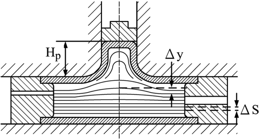
Schematic representation of geometrical configuration at protrusion stage.

In industrial applications, the minimal thickness ratio is 87.5%. Accordingly, the value of 90% for the thickness ratio at the top portion of the branch is decided in the adaptive control algorithm. For a larger contact length ratio at the top portion of the branch, a thinner tube is more likely obtained. Also the tube material is more difficult to flow into the branch cavity and separation is more likely to occur at the fillet part. Inversely, a smaller contact length ratio can get a thicker tube at the free bulge region. However, the top portion with a dome shape has to be cut off after hydroforming. A compromised value of 80% for the contact length ratio is determined from a series of simulation results.

Figure 7 shows the relationship between the axial feeding and internal pressures for different branch diameters. The tube diameter is fixed at D₀ = 60, whereas various branch diameters are chosen. Clearly, the internal pressure needed increases as the protrusion branch diameter D_p decreases. The instant for the beginning of the protrusion stage becomes earlier as D_p increases, because the material is easier to flow into the cavity for a larger protrusion branch diameter D_p.

Figure 7.

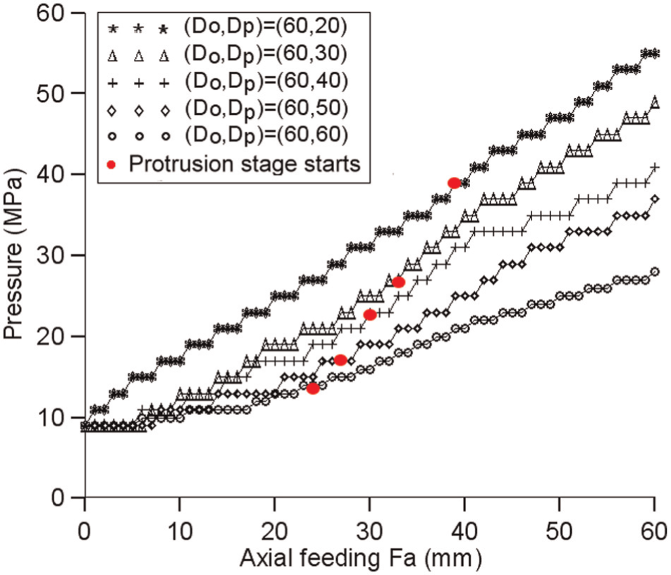
Relationship between axial feeding and internal pressures for different branch diameters.

Flow line net configurations during hydroforming without constraint at the branch top for different friction coefficients are shown in Figure 8. The outlet diameter ratio D_p/D_o is 30/60. The flow lines above symbol “o” are regarded as those flowing into the branch cavity, and those under symbol “x” are regarded as outside the branch cavity. The flow line net configurations show that the flow line number inside the branch cavity decreases with the increase in the friction coefficient. There are about 25% of the flow lines flowing into the branch cavity for µ = 0.2. The volume ratio from both sides into the branch cavity is twice the flow line number ratio. In order to prevent the tube material from accumulating at the entrance of the die fillet, one-half (50%) of the axial feeding speed has to be set as the CP speed for µ = 0.2. There are about 31%, 38%, and 45% of the flow lines flowing into the branch cavity for µ=0.15, 0.1, and 0.05, respectively. The volume ratio flowing into the branch cavity is a function of the coefficient of friction µ and the outlet diameter ratio D_p/D_o.

Figure 8.

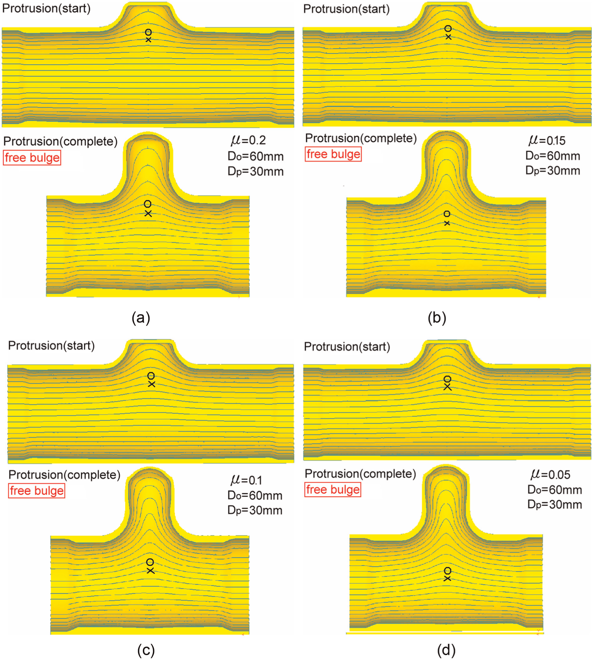
Flow line net configurations for different coefficients of friction. (a) µ = 0.2, (b) µ = 0.15, (c) µ = 0.1, and (d) µ = 0.05.

The speed ratio of the CP to the axial feeding is determined according to the ratio of the material volume flowing to the branch cavity to the whole tube volume, which varies with the branch diameter. An empirical relationship between the speed ratio, V_CP/V_AF, and the diameter ratio, D_p/D_o, can be obtained and expressed with a linear equation of V_CP/V_AF = 0.3 + 0.4(D_p/D_o).

Numerical results and discussion

The loading paths determined by the adaptive control algorithm using a pentagon die with different branch diameters are shown in Figure 9. The tube diameter is 60 mm. A friction coefficient of µ = 0.2 is set. The die fillet radius is set as 15 mm. The loading paths are divided into bulge and protrusion stages. The axial feeding speed is set as 0.06 mm/s, whereas the CP speed is set as 0.03, 0.034, and 0.038 mm/s for D_p = 30, 40, and 50 mm, respectively. Because more material volume is pushed into the die cavity for a larger branch diameter, accordingly, a faster CP speed has to be chosen.

Figure 9.

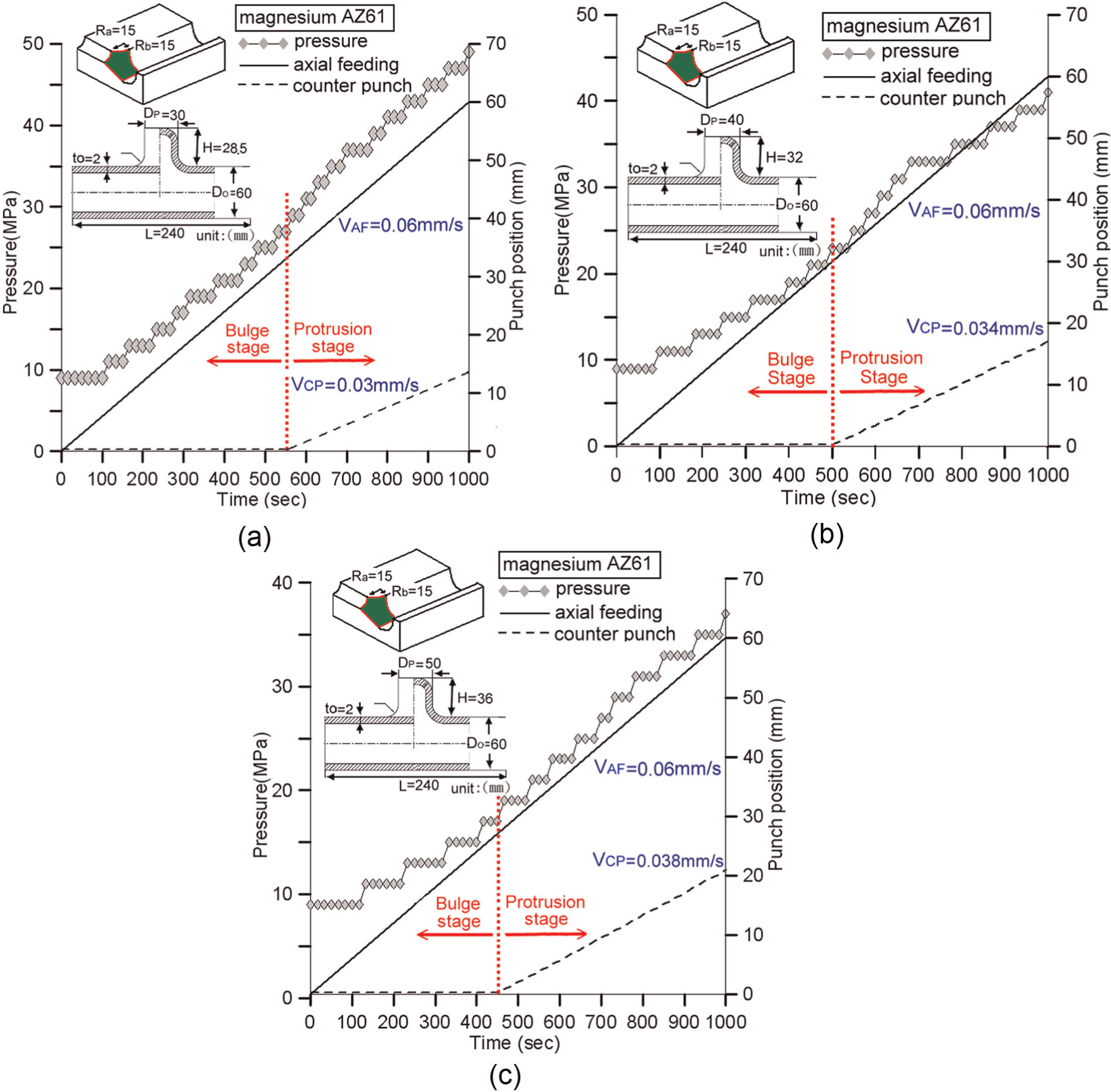
Loading paths obtained by adaptive control algorithm for different branch diameters. (a) D_p/D₀ = 30/60, (b) D_p/D₀ = 40/60, and (c) D_p/D₀ = 50/60.

The appearances of the hydroformed products for different branch diameters are shown in Figure 10. Clearly, sound products without any defects are obtained for all cases.

Figure 10.

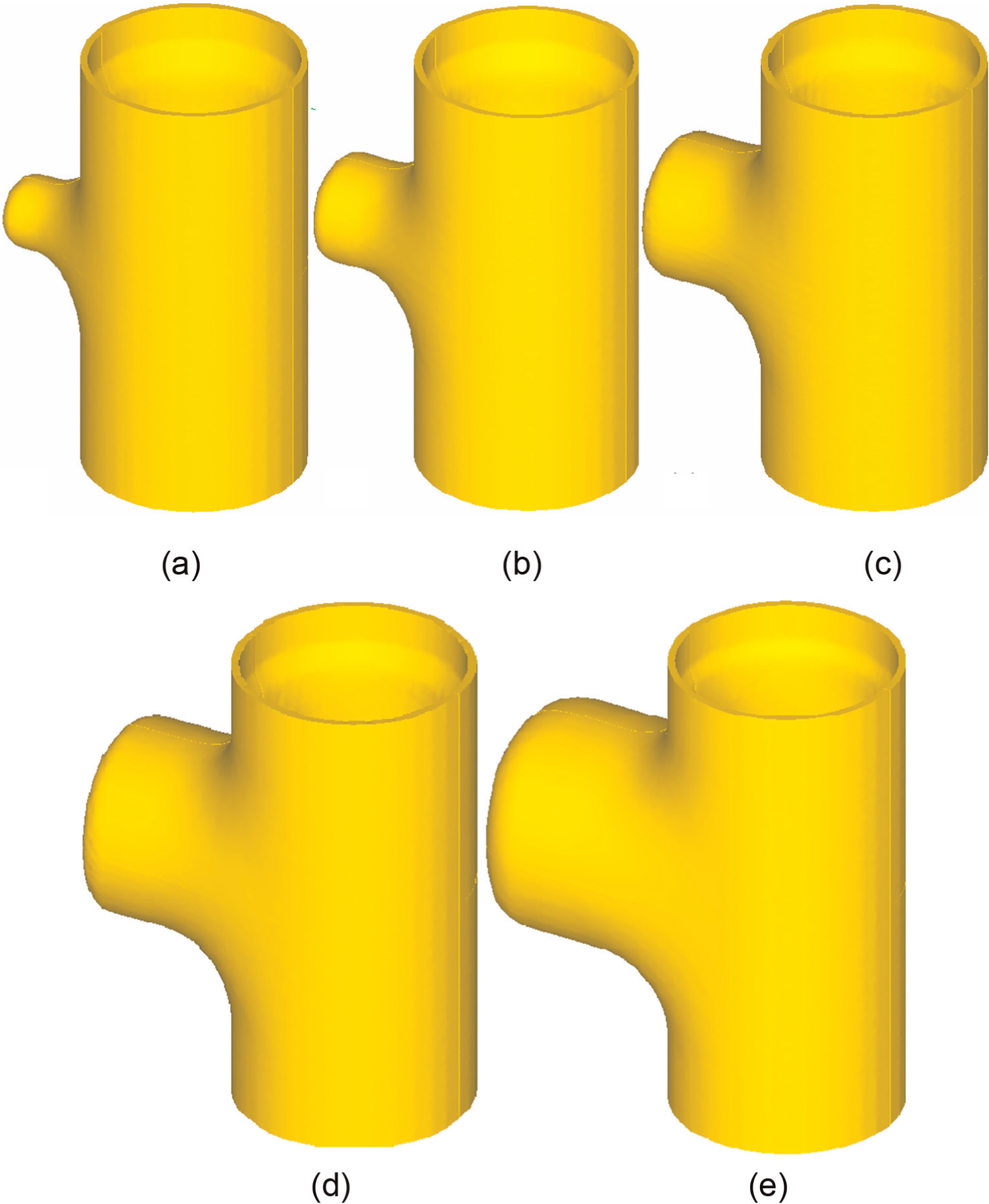
Appearance of hydroformed products for different branch diameters. (a) D_p/D₀ = 20/60, (b) D_p/D₀ = 30/60, (c) D_p/D₀ = 40/60, (d) D_p/D₀ = 50/60, and (e) D_p/D₀ = 60/60.

The thickness distributions at the upper part of the product for D_p/D_o=30/60 and D_p/D_o = 60/60 are shown in Figures 11 and 12, respectively. Figures 11(a) and (b) and 12(a) and (b) show the thickness distributions of the products just after the bulge and protrusion stages, respectively. The thickest parts occurred at the entrance of the die fillet. A 10-mm-long portion at both ends of the tube is used as oil sealing. Thus, the thickness remained the same after forming. The thinnest parts occurred at the top of the branch part. After the bulge stage, the thickness ratio t/t_o is about 90% for D_p/D_o = 30/60, and t/t_o is larger than 90% for D_p/D_o = 60/60. In this adaptive simulation algorithm, the thickness ratio at the branch top part being not smaller than 90% after the bulge stage is required. From Figures 11(b) and 12(b), it is known that after protrusion, the thickest parts occurred at around the entrance of the die fillet.

Figure 11.

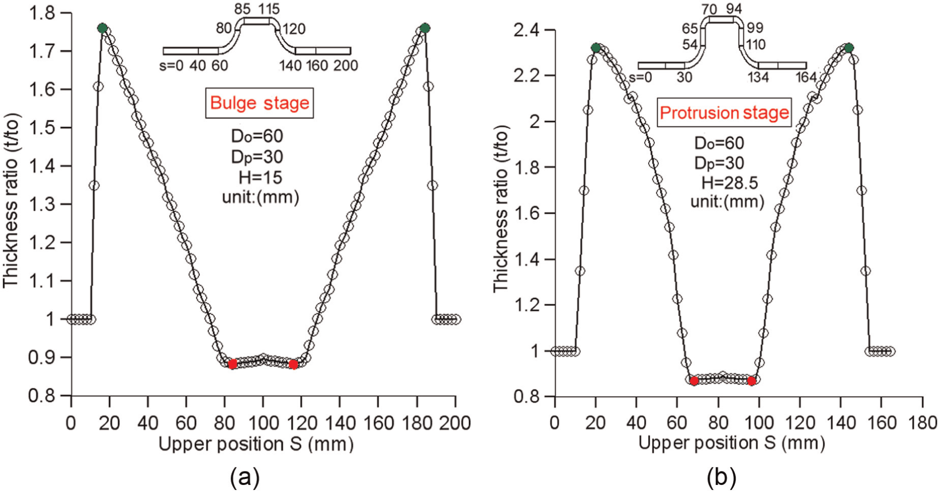
Thickness distributions at the upper part for D_p/D₀ = 30/60: (a) after bulge stage and (b) after protrusion stage.

Figure 12.

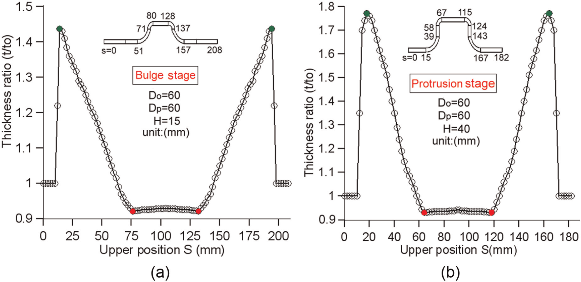
Thickness distributions at the upper part for D_p/D₀ = 60/60: (a) after bulge stage and (b) after protrusion stage.

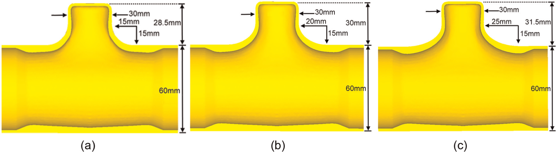
The longitudinal sections of the formed products with different fillet radii for D_p/D₀ = 30/60 are shown in Figure 13. In Figure 13(a), the die fillet surface is regarded as a circular arc of R_a = R_b = 15 mm. In Figure 13(b) and (c), the fillet surface is regarded as an elliptical arc of R_a/R_b = 20/15 and 25/15, respectively. Generally, there is no big difference in the product profiles with circular and elliptical arcs. However, the formable protrusion height with an elliptical arc is larger than that with a circular arc.

Figure 13.

Longitudinal sections of the formed product with different fillet radii: (a) R_a/R_b = 15/15, (b) R_a/R_b = 20/15, and (c) R_a/R_b = 25/15.

The thickness distributions at the upper part of the formed product with different fillet radii are shown in Figure 14. The thickest parts occurred at around the entrance of the die fillet. The thickness at the both ends of the tube did not change because these parts are used as oil sealing. The thinnest part occurred at the top of the branch. The total length at the upper part with an elliptical arc is larger than that with a circular arc, because a larger protrusion height is obtained with an elliptical arc.

Figure 14.

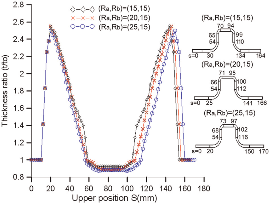
Thickness distribution at the upper part for different fillet radii.

Experiments of T-shaped hydroforming processes

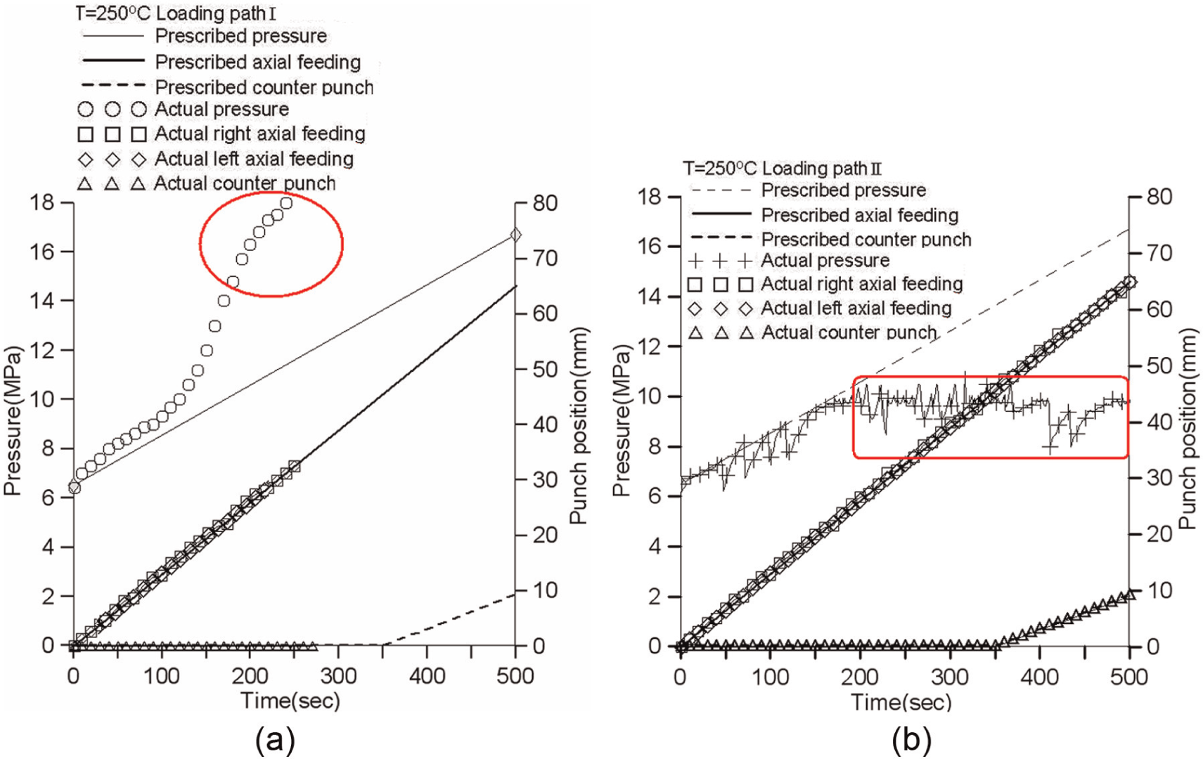
Experiments of T-shaped hydroforming processes were conducted using a self-designed hydroforming machine. ¹⁸ The forming temperature is 250 °C. One kind of silver grade anti-seize grease containing graphite and calcium oxide was used for lubrication at the interface between the tube and die. A pentagon die was designed for a tube of 53.4 mm in diameter, 280 mm long, and 2.08 mm thick. The branch diameter is 26.7 mm. Three kinds of loading paths were used in the experiments. The first two are shown in Figure 15(a) and (b). The prescribed loading path is obtained by the adaptive control algorithm. From Figures 15(a) and (b), it is known that the actual movement of the axial feeding and CP faithfully followed the prescribed positions. However, the actual input internal pressure profile was higher than the prescribed pressurization curve in loading path I and was lower than the prescribed one in loading path II.

Figure 15.

Analytical and experimental loading paths: (a) loading path I and (b) loading path II.

The warm forming temperatures for magnesium alloys range approximately from 150 °C to 300 °C. At lower temperatures, magnesium tube material can deform with a higher rigidity, less tube material accumulates at the guiding zone, and accordingly, a better thickness distribution can be obtained. The demerit for forming at a lower temperature is that a larger internal pressure is required. Considering the capacity of the hydroforming test machine used in the experiments, a higher temperature of 250 °C was selected in the THF experiments.

A constant friction coefficient of 0.2 is adopted in the FE simulation to correspond to the warm forming conditions with the lubricant of one kind of silver grade anti-seize grease. The friction coefficient at the tube–die interface is a function of forming pressure, forming temperature, forming speed, lubricant, and so on. From the friction tests at elevated temperatures, ²⁰ the variation of the friction coefficient is about 0.1–0.2. For simplicity, a constant friction coefficient of µ = 0.2 is assumed in the FE simulation.

The appearance of the formed product using loading paths I and II is shown in Figure 16(a) and (b), respectively. For loading path I, because of an excessively large pressurization, bursting occurred at the branch part, as shown in Figure 16(a). For loading path II, because of an excessively small pressurization, the contact length ratio L_cp/D_p was less than 80% and the tube could not fill up the corner of the branch.

Figure 16.

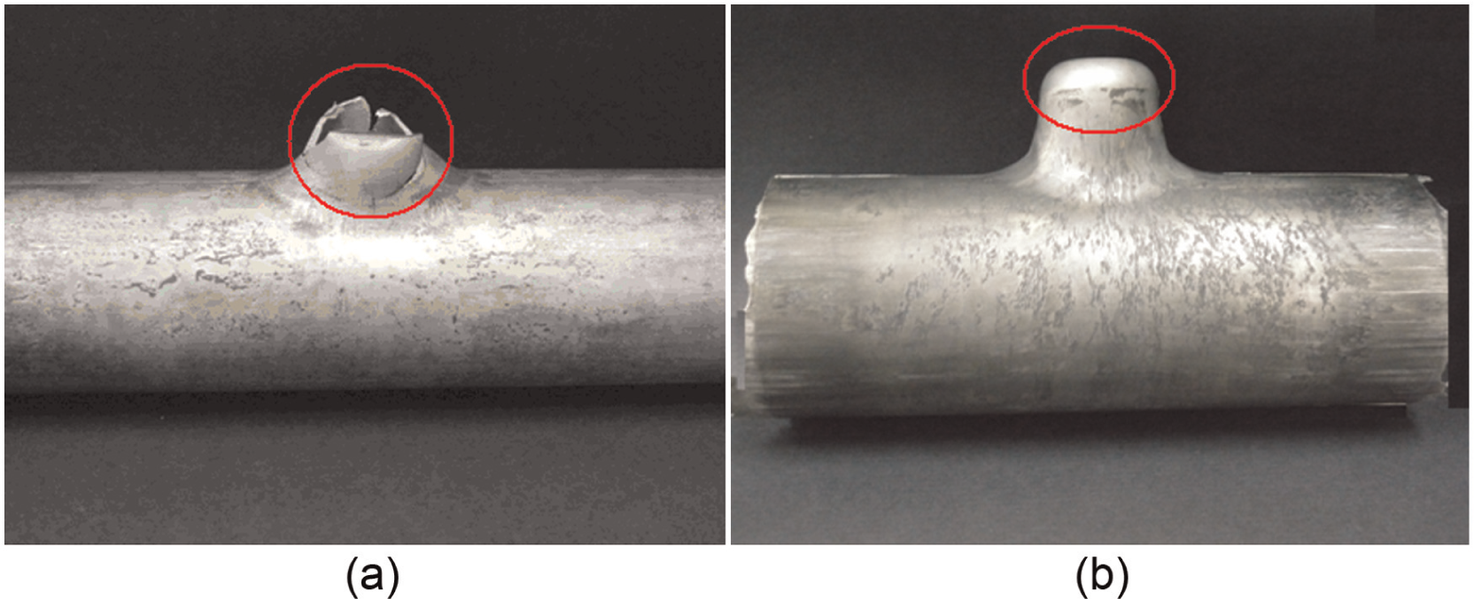
Appearance of formed product using different loading paths: (a) loading path I and (b) loading path II.

During the first time of the experiments, the electromagnetic relief valve that used to release the forming pressure did not work properly, the internal pressure became larger than the prescribed pressurization profile, and, eventually, it resulted in bursting at the branch part. During the second time of the experiments, the pressure intensifier used to increase the forming pressure did not work properly, the internal pressure became smaller than the prescribed pressurization profile, and, eventually, the tube material failed to fill up the corner of the branch.

Figure 17(a) and (b) shows loading path III and the longitudinal section of the obtained product, respectively. Because the internal pressure was controlled manually, fluctuation in the pressurization curve was observed. The average of the experimental pressurization curve was slightly smaller than the prescribed one, because the response of the intensifier pump became slower at higher pressures. Nevertheless, the pressurization is quite close to the prescribed one. Accordingly, a sound product with L_cp/D_p larger than 80% and the thickness ratio t/t_o at the top position larger than 90% was obtained. Generally, the analytical flow line configuration is quite similar to the actual one.

Figure 17.

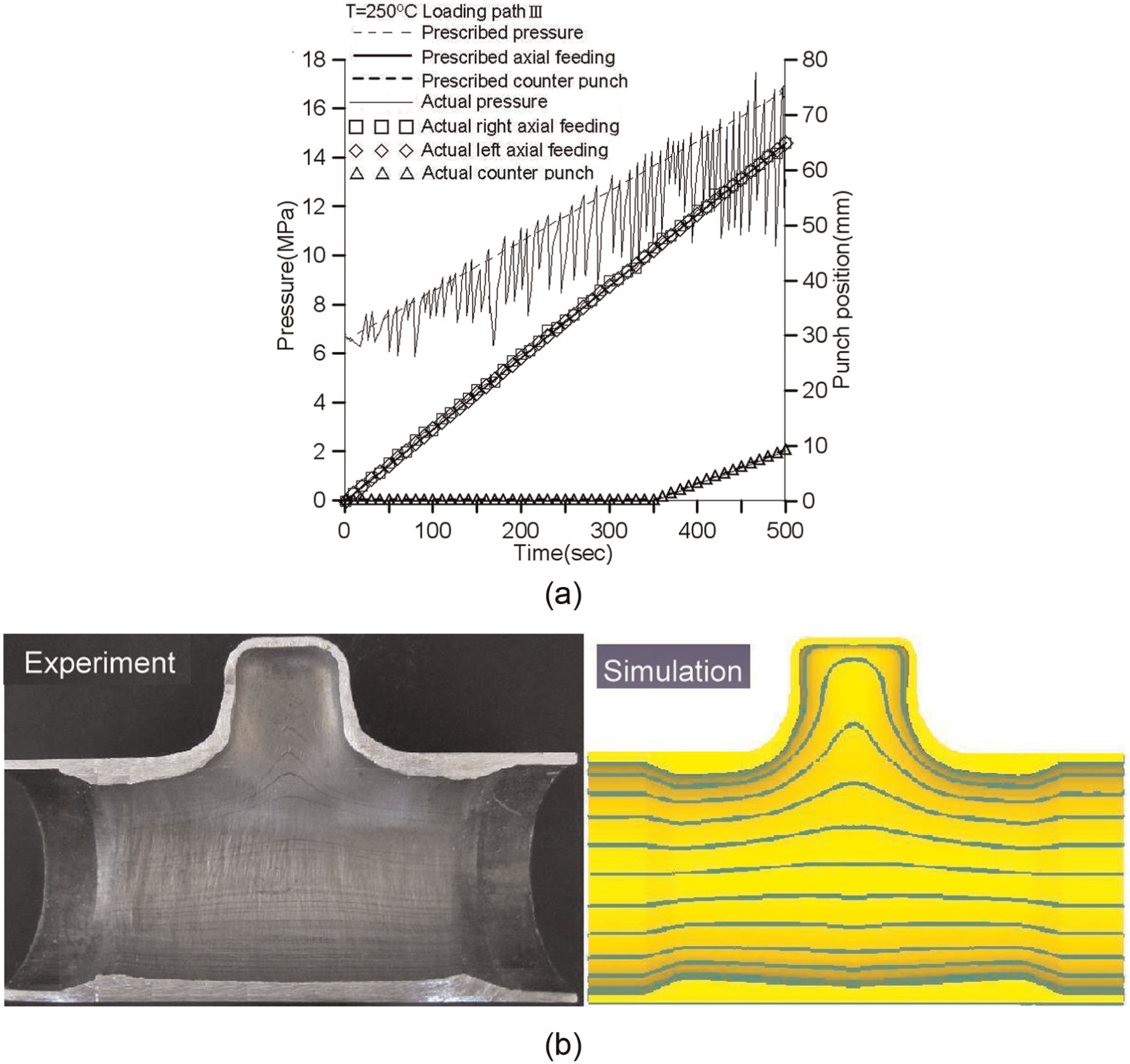
Experimental results with loading path III: (a) loading path III and (b) longitudinal section of formed product.

Conclusion

In this study, an adaptive simulation algorithm for the loading paths of T-shaped hydroforming was proposed to determine the internal pressurization and the axial and CP speeds during THF with different outlet diameters. The FE analysis was used to simulate the flow pattern of the tube during the THF process. The analytical flow line net configurations of the tube were utilized to determine the speed ratio of the CP to the axial feeding in the protrusion stage. Appropriate loading paths for different outlet diameters were determined using the proposed adaptive control algorithm and sound products without any defects were obtained. The protrusion heights and thickness distributions of the formed product with circular and elliptical arcs at the die fillet were compared. Experiments of T-shaped warm hydroforming of magnesium alloy AZ61 tubes with a 1/2 outlet diameter ratio were conducted. Sound products with a branch height of 25 mm and a minimum thickness of 90% of the initial thickness were obtained. From the comparisons of the product shape and the flow line net configurations between the analytical and experimental values, the validity of the analytical models was verified.