Process capability indices have been widely used in the manufacturing industry to provide numerical measures for process potential and process performance. However, from the perspective of improving process quality, there is a significant amount of process information that cannot be conveyed with a single index. Therefore, a single index does not have the ability to represent distinct problems in process performance or to provide the production department with sufficient information to make improvements. Thus, we applied an accuracy index and a precision index capable of reflecting the degree of deviation from target values and the degree of variance and incorporated the quality-level concept of the six-sigma model to develop a process quality-level analysis chart capable of analyzing the process capabilities of multiple quality characteristics. In addition to being able to directly identify the quality levels for various quality characteristics, the process quality-level analysis chart also provides recommendations for improvement of all quality-level regions to serve as a reference for production departments. Mathematical programming was used to develop a statistical hypothesis testing model to assist production departments in confirming the effectiveness of implemented improvements. This was achieved through derivation of a joint confidence interval for and from Boole’s inequality. From this, we obtained the upper and lower limits of the for and . Finally, we also applied the proposed approach to a case study of a five-way pipe process.
Manufacturing processes are subject to the influences of multiple factors, all of which increase the difficulty of the process quality evaluation. In recent years, many novel evaluation methods have been introduced to enhance process analysis and problem solving through definition of an effective production capability index. A considerable amount of research has focused on process capability indices (PCIs) as convenient and effective tools for measuring process performance to assist in quality assurance and purchasing decisions.1–6 Using PCIs, production departments can trace and improve quality characteristics. Consequently, these indices have been widely applied in the automated manufacturing, semiconductor, and packaging industries.
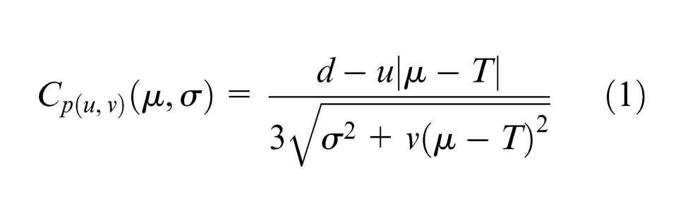
In the last two decades, numerous statisticians and quality engineers have investigated PCIs with the aim of improving the assessment of both process potential and performance.7–18 These indices, including the basic forms , , , and , are appropriate measures for processes with two-sided specifications and have become popular unitless measures for determining whether a process is capable of reproducing items that meet the quality requirements preset by the product designer. The rule for the general form is larger the better. In view of this, Vännman and Kotz19 proposed a class of capability indices depending on two nonnegative parameters, and , defined as follows
where is the process mean, is standard deviation (overall process variability), is the half-length of the specification interval, is the target value, and . Thus, the above-mentioned four basic indices can be considered as special cases of equation (1). It is easy to verify that , , , and .
Some of the desirability of these indices originates from their unitless nature. In terms of management and marketing, this characteristic of PCIs provides production departments with a simple and convenient basis for determining process performance. As a result, they can serve as a common language among management departments, sales departments, and customers, thereby facilitating product sales and the receipt of orders. However, there is a significant amount of process information that cannot be conveyed with a single index. When requirements specified by customers have not been met, a single index does not have the capacity to represent distinct influences on process performance or to provide the production department with a sufficient reference to make improvements.
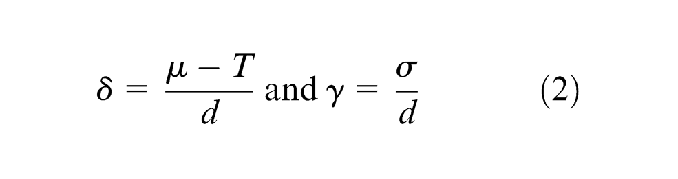
This same point was made by Deleryd and Vännman,20 who stressed that PCIs, such as that depicted in equation (1), which combine information about closeness to a target (accuracy) and process spread (precision) into representation by a single number, pose major drawbacks. For instance, if the process is found noncapable, quality engineers must know whether this noncapability is caused by an inaccurate process mean, too much deviation, or a combination of these two factors. Thus, considering as the accuracy index, which measures the degree of process centering, and as the precision index, which measures the degree of process deviation, we define the process as follows
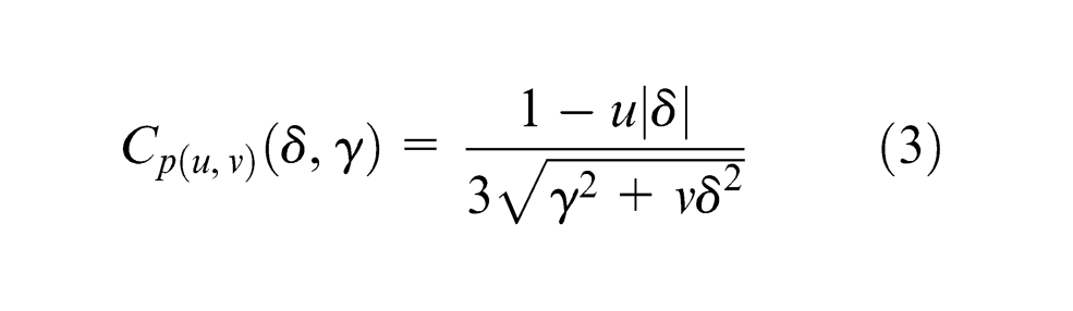
Based on the suggestions of Deleryd and Vännman,20 a number of researchers have converted PCIs into functions of the parameters and to measure and evaluate process capability.21–26 Their objective was to assist production departments in quickly analyzing the process yield of various quality characteristics, the degree to which they deviated from target values, and their degree of variance, so that personnel could effectively impose improvement measures. To this end, equation (1) can be redefined and rewritten as
Similarly, the basic indices , , , and can be considered as special cases of the index in equation (3) by letting or 1, and or 1. In recent years, the six-sigma quality management model has effectively reduced the defect rates of product manufacturing. At a six-sigma quality level, the number of defective products reduces to only 3.4 in every million products. For this reason, the model has been widely applied in the manufacturing industry as a method of cost reduction. Previous studies27–30 employed different capability indices to derive the relationship between process capability and six-sigma quality levels to assess and determine process performance. However, when the values of different PCIs are equal, the process capabilities and quality levels that they imply for the quality characteristics differ, which can inconvenience product departments during application.
In summary, accuracy and precision indices have an advantage over conventional PCIs in the evaluation of process levels. Therefore, we applied the concept of quality levels in the six-sigma model to develop a process quality-level analysis chart (PQLAC) based on precision index and accuracy index . The proposed approach enables plotting several nominal-the-best quality characteristics on a single analysis graph. This graphic representation clearly shows the extent to which the quality characteristics have deviated from their target values (accuracy) and the degree of variance in the quality characteristics (precision). In addition to creating a chart to enable direct evaluation of the process quality levels of different quality characteristics, we collected reference material from expert personnel to assist in the improvement of the process capabilities. Finally, we developed a pre- and post-improvement hypothesis testing model with which production departments can assess the effectiveness of their improvement efforts.
Relationship among quality level, δ, γ, and process yield
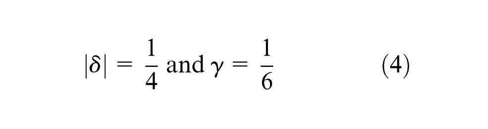
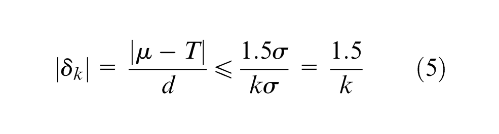
As mentioned above, the accuracy index primarily measures the extent to which the process mean has deviated from target value T. closer to 0 indicates a smaller deviation in the process mean and a higher degree of accuracy. The precision index represents the degree of variance in the process; a smaller value indicates a lower degree of standard deviation and a higher degree of precision. Definitions of the two indices are presented in equation (2). Pearn and Chen31 and Chen et al.32 stated that to achieve a six-sigma quality level, the process must present a mean deviation of from the target value and a standard deviation of . It is apparent that when the quality level of the process reaches six sigma and if the process mean displays a left offset of from the target value and , then . Thus, equation (2) can be expressed as
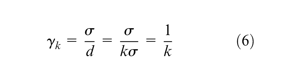
For the sake of generality, let denote the process accuracy when the quality level reaches sigma and let represent the process precision when the quality level reaches sigma. Therefore, when the quality level of the process reaches sigma, and can be expressed as follows
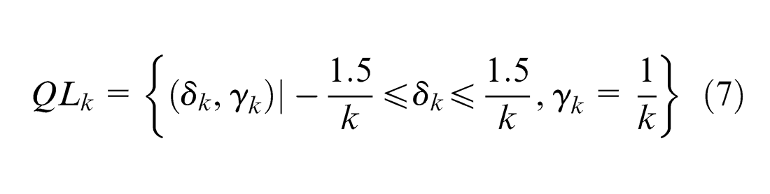
Thus, in addition to using equations (5) and (6) to evaluate accuracy and precision of the process for quality characteristics, we can also determine whether the process attains the sigma quality-level set by the production department. The constraint for the quality-level measurement region is therefore
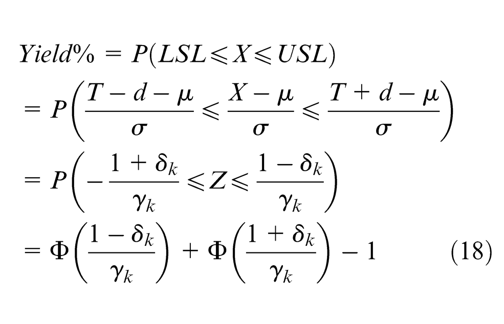
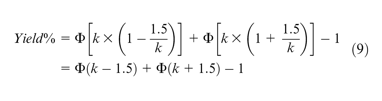
For processes with two-sided specification limits, the process yield can be calculated as , where is the cumulative distribution function of the quality characteristic , is the upper specification limit, and is the lower specification limit. On the assumption of normality, process yield can be expressed as follows
By substituting equations (5) and (6) into equation (8), we can derive the relationship between process yield and quality levels
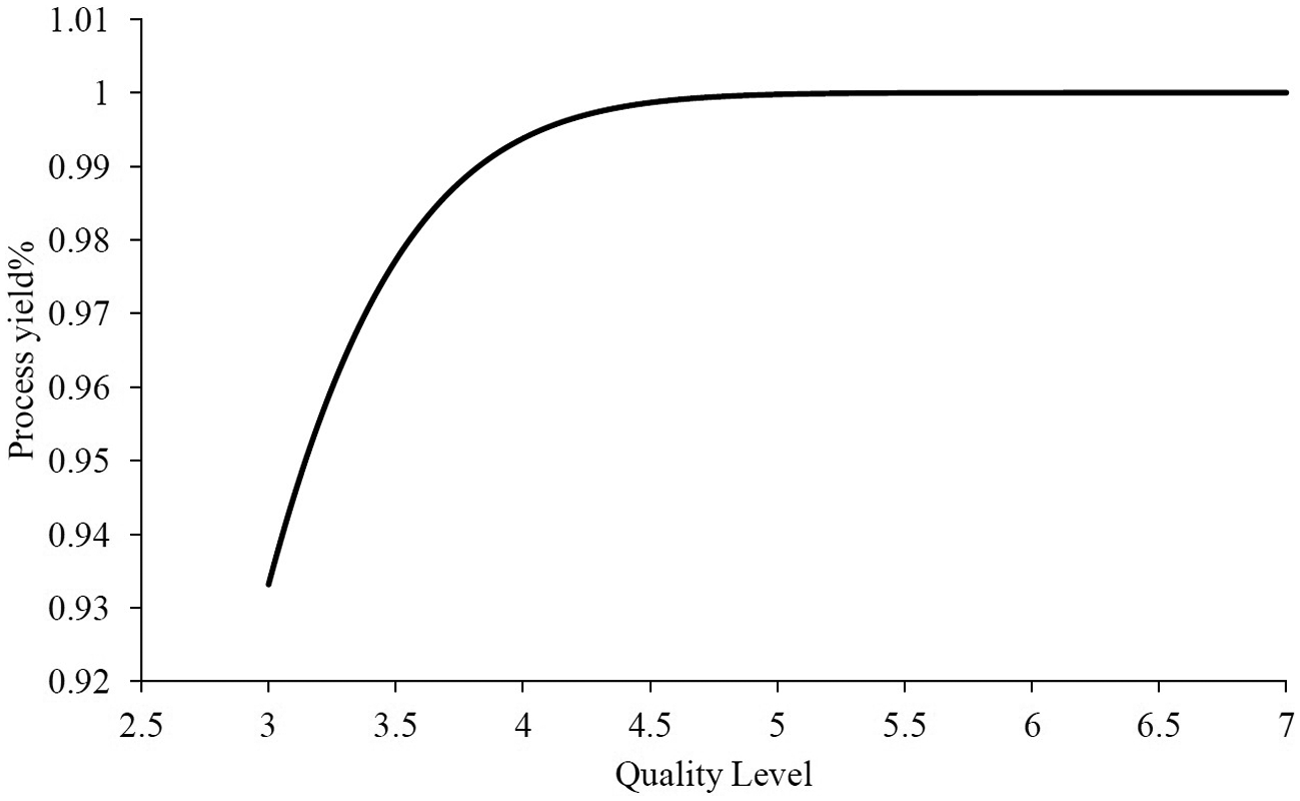
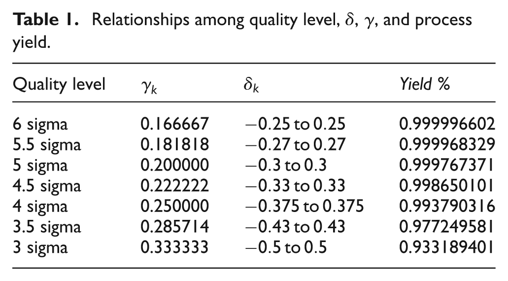
A comprehensive view of the content above shows that when production departments set a stronger regulation of quality levels, process yield increases (as shown in Figure 1), and accuracy and precision are greater. Table 1 presents the relationships among quality level, , , and process yield %.
Relationship between quality level and process yield.
Relationships among quality level, , , and process yield.
Quality level
Yield %
6 sigma
0.166667
0.999996602
5.5 sigma
0.181818
0.999968329
5 sigma
0.200000
0.999767371
4.5 sigma
0.222222
0.998650101
4 sigma
0.250000
0.993790316
3.5 sigma
0.285714
0.977249581
3 sigma
0.333333
0.933189401
PQLAC
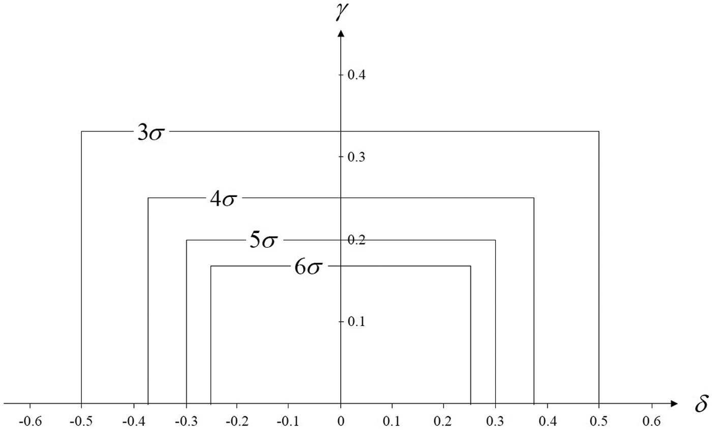
As discussed above, the accuracy index and the precision index can effectively present the extent to which process quality characteristics have deviated from target values and their degree of variance. Smaller values in both indices indicate that the process yield and quality levels of the quality characteristic are better. To simultaneously evaluate the process performance and quality levels of multiple nominal-the-best quality characteristics, we developed a PQLAC with the accuracy index on the horizontal axis and the precision index on the vertical axis, as shown in Figure 2. The PQLAC can be used to determine the process performance of various quality characteristics and allows production departments to track and improve quality characteristics with poor process capabilities, thereby allowing the enhancement of overall production quality to meet customer needs.
Process quality-level analysis chart (PQLAC).
In this section, we detail the application of the PQLAC. We first assume that the process performance of a given quality characteristic has already achieved the three-sigma quality level, but it does not exceed the four-sigma quality level. Obviously, at present, the process yield of the quality characteristic is greater than 0.933189 and smaller than 0.993790 (i.e. ). When the factory produces 1 million products every time, the number of the defective products ranged between 6210 and 66810 based on the above equation. Hence, the production costs and materials of these defective products not only incur considerable losses but also increase rework costs for enterprises, further undermine the market competitiveness of the company. For this reason, the production department must actively analyze and identify the causes of this poor process performance and then adopt relevant improvement measures to enhance the process level so that the quality characteristic can be increased to the ideal six-sigma quality level, as shown in Figure 3, allowing for the reduction of the defect rate and consequent costs. Following analysis and identification, improvements in each quality-level region are carried out according to the reference provided by expert personnel. These recommendations are displayed in Table 2.
When a quality characteristic falls within the quality-level regions of A or B, the process displays sufficient process precision but insufficient accuracy. Clearly, the process mean of the quality characteristic has significantly deviated from the target value (too small or too large); the possible causes of the poor process performance include improper operation, undue processing, and incorrect parameter settings. Therefore, the production department should review operation procedures and adjust parameter settings to increase the accuracy of the process and improve the quality level to within the six-sigma control region.
When a quality characteristic falls within the quality-level region C, the process displays sufficient process accuracy but insufficient precision. There is a high degree of variance in the quality characteristic, and the possible causes include poor quality of raw materials, unstable processing quality, and old processing machines. As a result, to move the quality level to within the six-sigma control region, the production department should perform stricter inspections, impose greater control measures on materials, and improve or replace processing machines. Relatively speaking, enhancing the precision of the process increases costs.
When a quality characteristic falls within the quality-level regions of E or F, both the precision and accuracy of the process are insufficient. Therefore, the deviation of the process mean and the degree of variance in the quality characteristic are too large, and the possible causes for this include the causes identified in the two previous points. In-depth investigation is required as well as corresponding improvement measures to enhance the precision and accuracy of the process and satisfy the ideal six-sigma quality level.
Application and analysis of PQLAC.
Database of expert advice
Quality area
State of performance
Possible cause
Recommended improvement
Improvement cost
A and B
Sufficient process precision but insufficient accuracy
Improper operation
Review operation procedures and establish standard operating procedures (SOPs)
Low
Undue processing
Intensify personnel training and selection procedures and establish a reward and penalty system
Incorrect machine parameter settings
Adjust machine parameters and institute regular checks
C
Sufficient process accuracy but insufficient precision
Poor quality of raw materials
Enhance inspection and control of raw materials and select suppliers with quality guarantees
High
Unstable processing quality
Regularly inspect processing tools and confirm their processing performance and lifespan
Old processing machines
Regularly replace old machines
E and F
Both accuracy and precision insufficient
See defects in A, B, and C
See recommendations for A, B, and C
Bigger than A and B
Hypothesis testing model for process improvement effectiveness
The PQLAC can assist the production department in the identification of critical-to-quality characteristics with poor process capabilities. Based on the accuracy index and the precision index , factors influencing the performance of the process can be systematically analyzed, thereby enabling the improvement of quality levels. However, once corresponding improvement mechanisms have been implemented, the production department must confirm whether the improvements were as effective as anticipated and the target quality levels demanded by customers have been reached. We developed the hypothesis testing method used in the field of statistics through the derivation of a joint confidence interval for and based on Boole’s inequality. The joint confidence interval for and can be expressed as
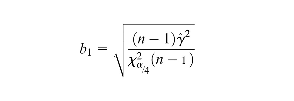
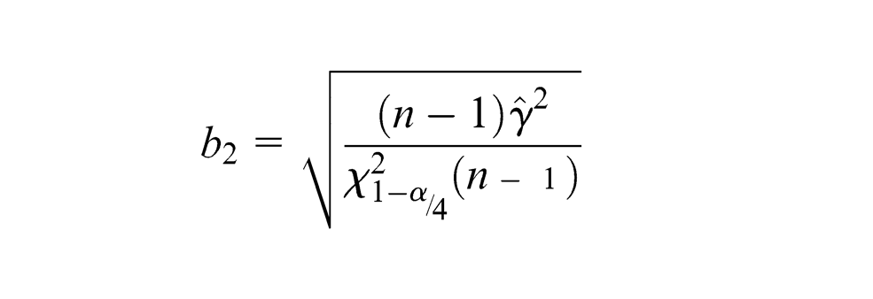
When , we can obtain the Cartesian product from the inequality above, which defines set region as
where
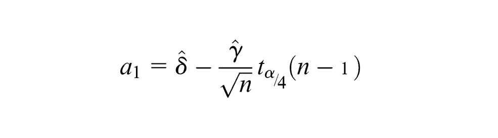
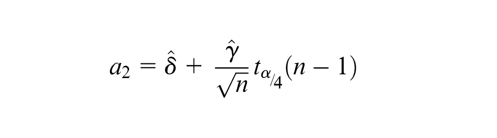
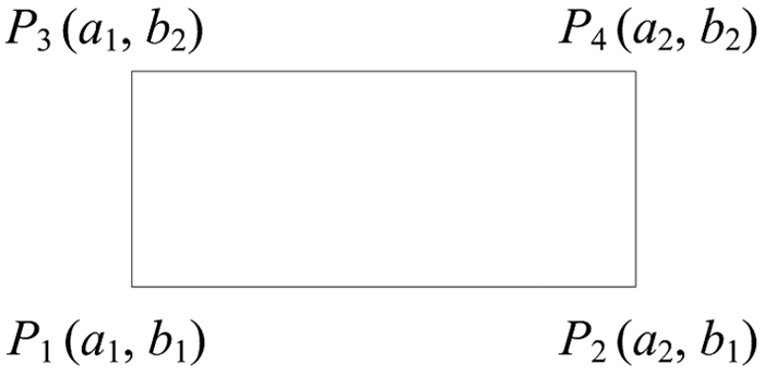
Using the four values above, we construct the joint confidence region for and , that is, set region . The schematic diagram is shown in Figure 4.
Schematic diagram of set region .
In terms of practical application, the of each quality characteristic has a probability of falling within the joint confidence region. In fact, the distance between and the origin represents the quality level of the quality characteristic. Therefore, the closer and are to 0, the smaller is and the higher the precision and accuracy of the process. This also implies that the quality level of the quality characteristic in the process is higher. In contrast, the further and are from 0, the lower the quality levels. For the sake of generality, we set the six-sigma quality level as the measurement standard for improvement effectiveness. Using mathematical programming, we obtained the upper and lower limits of a confidence interval for and to develop a statistical hypothesis testing model to determine the effectiveness of improvement measures.
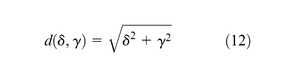
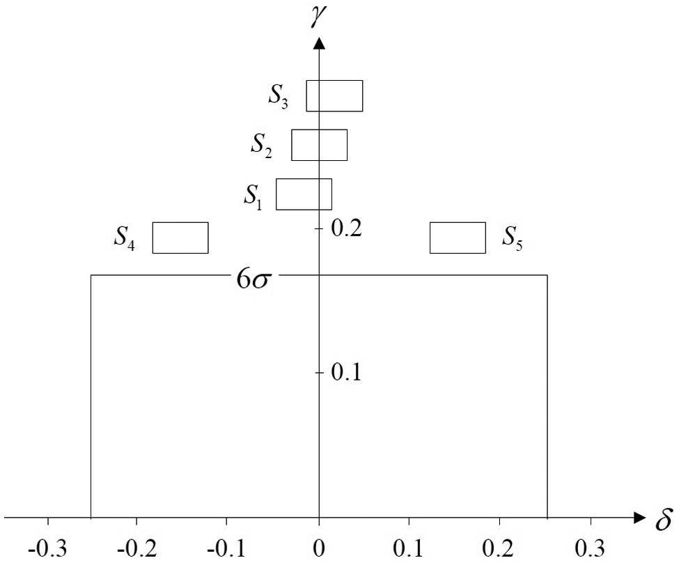
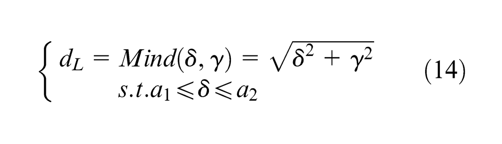
We employed the distance between and the origin as the target function, as shown in equation (12), and the set region as the region of feasible solutions to derive the maximum and minimum values and thus the upper and lower limits of the confidence interval, as shown in Figure 5.
Schematic diagram to solve upper and lower limits of the confidence interval for and .
Lower confidence limit
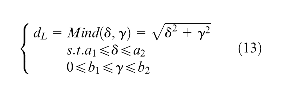
As established previously, the mathematical programming model for the lower limit of the confidence interval for and can be written as
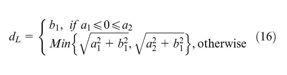
However, as we used the distance between and the origin as the target function, it is clear that the distance between the origin and the in the feasible region closest to the origin is the lower confidence limit. Figure 5 shows that the line segment in the feasible region is the closest to the six-sigma quality-level region. The lower limit of the confidence interval for and must therefore be above line segment . As a result, we need not discuss the entire feasible region for the lower limit of the confidence interval for and . This lower limit can be rewritten as
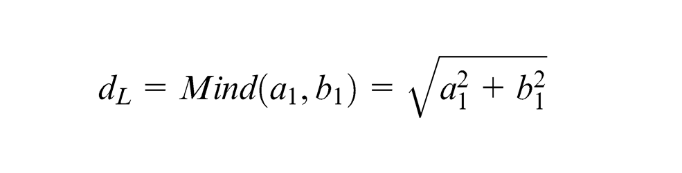
When , or for the cases , , and in Figure 5, the minimum value of the target function can be obtained at ; thus, the lower confidence limit is
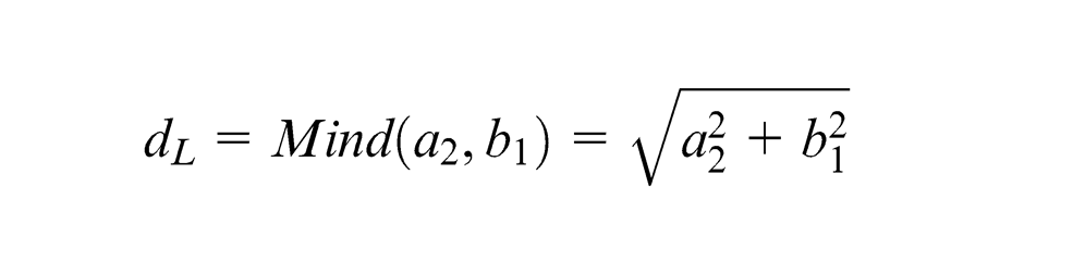
When , then case in Figure 5 occurs, indicating that the minimum value of the target function can be obtained at ; thus, the lower confidence limit is
When , then case in Figure 5 occurs, indicating that the minimum value of the target function can be obtained at ; thus, the lower confidence limit is
Upper confidence limit
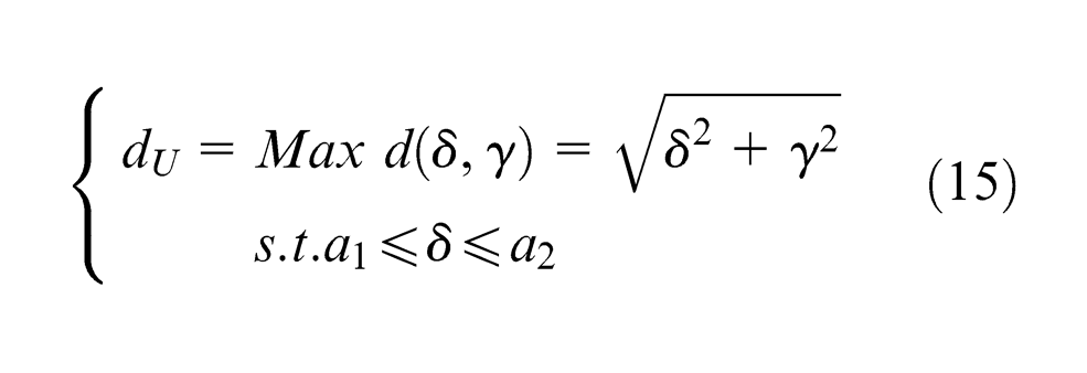
Similar to previous section, line segment in the feasible solution region is the furthest from the six-sigma quality-level region. Therefore, the mathematical programming model for the upper limit of the confidence interval for and is
When , case in Figure 5 occurs, indicating that the maximum value of the target function can be found at or ; thus, the upper confidence level is
When , then , which indicates cases and in Figure 5, implying that the maximum value of the target function can be found at ; thus, the upper confidence level is
When , then , which indicates cases and in Figure 5, implying that the maximum value of the target function can be found at ; thus, the upper confidence level is
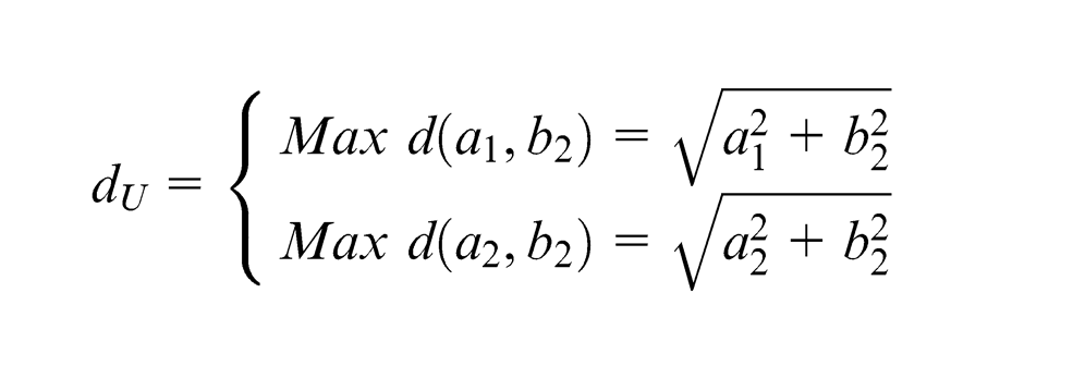
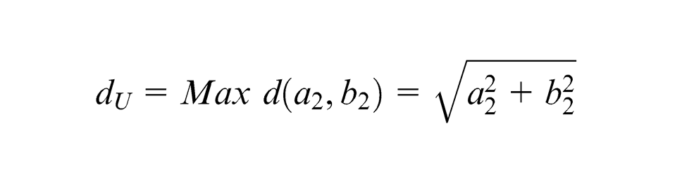
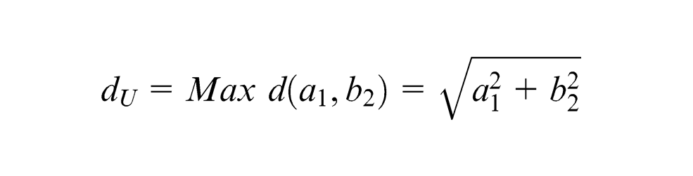
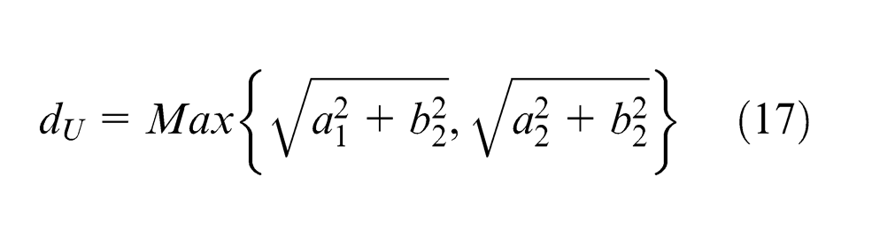
In summary of the derivations above for the upper and lower limits of a confidence interval for and , we collated the optimal solutions for upper and lower confidence limits as follows
Testing model and evaluation criteria
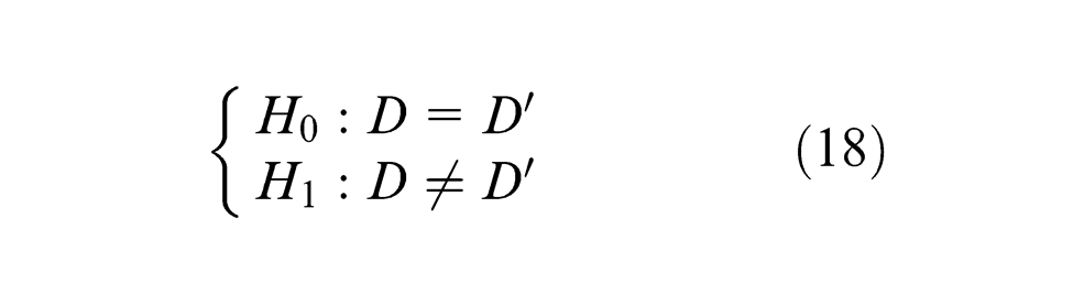
Making use of the upper and lower limits presented in equations (16) and (17), we let the upper and lower limits before and after improvement measures be and , respectively. Thus, the statistical hypothesis testing model for the effectiveness of process improvement is
The evaluation criteria of these sets of limits are as follows:
When , we do not have sufficient proof to reject . In other words, the difference between the quality levels before and after improvement measures was not significant. Therefore, the production department should continue to actively track and analyze process operations and formulate optimal measures to deal with the poor process performance of the quality characteristic in question.
When , we have sufficient proof to reject . Determining the degree of improvement effectiveness depends on the following conditions:
When , a significant difference is shown in quality after improvement measures have been carried out. Nevertheless, the production department should continue to monitor and control the production procedures to maintain acceptable quality levels. Maintaining the current improvement effectiveness will benefit the company’s competitiveness in the industry.
When , quality performance has decreased following improvement measures. This shows a severe error; the production department should terminate current measures and reexamine tracking and analysis to identify the causes of poor performance. New improvement measures should then be formulated to enhance quality levels; otherwise, an excess number of defective products will be produced, incurring more costs and damaging the continued development and competitiveness of the company.
Case study
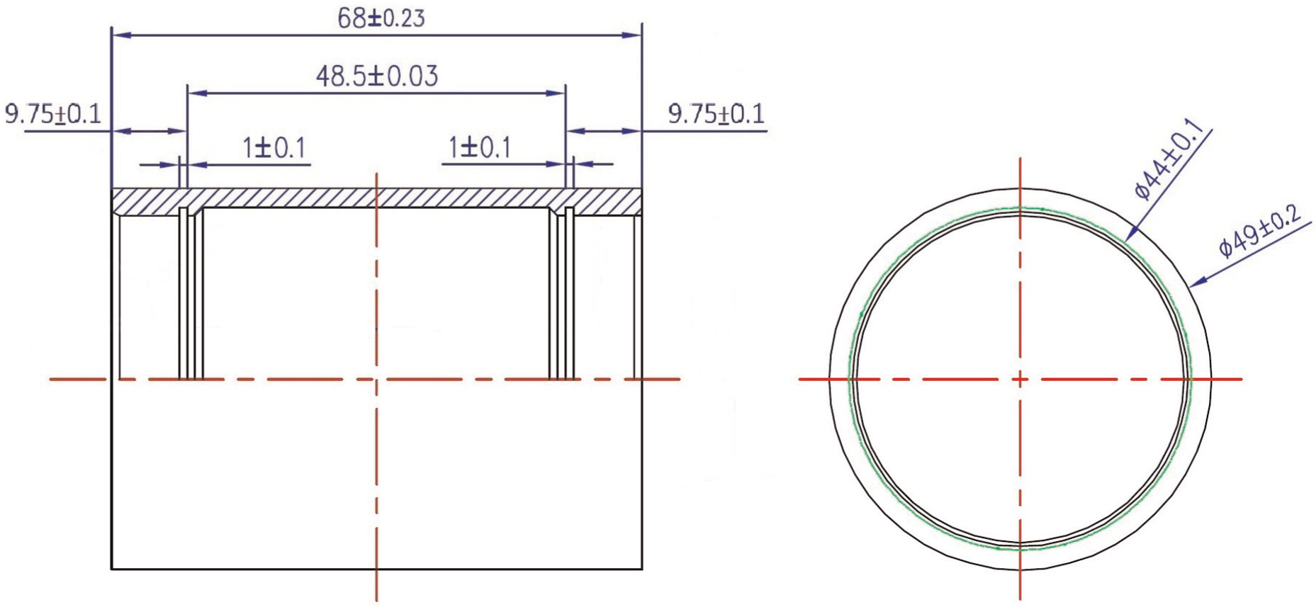
In this section, we consider a case study to demonstrate the proposed PQLAC and the testing model. The selected case is the manufacturing process of a five-way pipe, which is an important component in the production of bicycles. The structure of a specific five-way pipe is shown in Figure 6, and the specifications of its quality characteristics are presented in Table 3; data were taken from a factory located in Taichung, Taiwan. All of the key quality characteristics of the five-way pipe are nominal-the-best specifications.
Structure of five-way pipe.
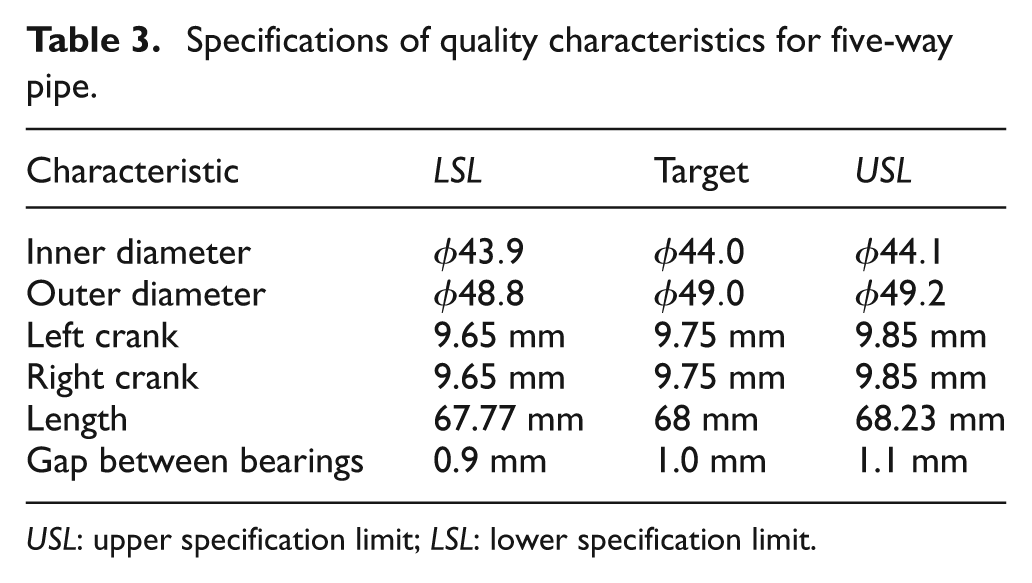
Specifications of quality characteristics for five-way pipe.
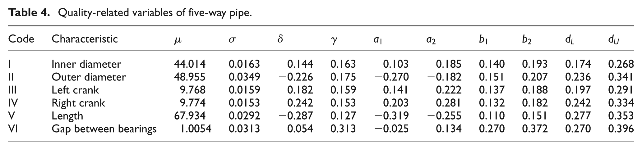
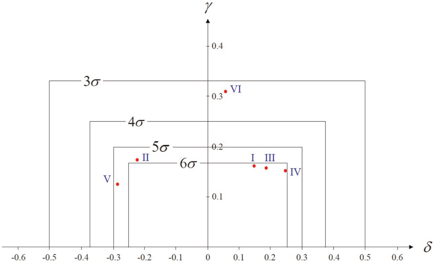
We considered a random number of samples—100—from a stable (under statistical control) process and measured six product quality characteristics. For the sample, the Kolmogorov–Smirnov test for normality confirmed a . That is, it is reasonable to assume that the process data collected from the factory are normally distributed. The calculated sample mean; sample standard deviation; accuracy index ; precision index ; points of joint confidence interval, , , , ; and 95% lower confidence limit and upper confidence limit are presented in Table 4. Five pairs of and values are plotted on the proposed PQLAC in Figure 7, clearly representing the process status of each in-process quality characteristic in a single tool. As can be seen from this figure, it is easy to determine their quality level and process performance.
Quality-related variables of five-way pipe.
Code
Characteristic
I
Inner diameter
44.014
0.0163
0.144
0.163
0.103
0.185
0.140
0.193
0.174
0.268
II
Outer diameter
48.955
0.0349
−0.226
0.175
−0.270
−0.182
0.151
0.207
0.236
0.341
III
Left crank
9.768
0.0159
0.182
0.159
0.141
0.222
0.137
0.188
0.197
0.291
IV
Right crank
9.774
0.0153
0.242
0.153
0.203
0.281
0.132
0.182
0.242
0.334
V
Length
67.934
0.0292
−0.287
0.127
−0.319
−0.255
0.110
0.151
0.277
0.353
VI
Gap between bearings
1.0054
0.0313
0.054
0.313
−0.025
0.134
0.270
0.372
0.270
0.396
PQLAC for five-way pipe.
The PQLAC allows for quick evaluation of whether or not the quality performance meets the required minimum five-sigma level. The five-sigma level is within the contours of and . Clearly, the plotted points I, II, III, IV, and V lie inside the area of . In contrast, the plotted point VI lies outside the set area. The excessive process variance in point VI is, therefore, the primary cause of insufficient process levels. Thus, quality improvement efforts focused on point VI should be based on the reduction of process variance. In this endeavor, the production department can refer to the expert recommendations in Table 2 to effectively enhance the performance of the process associated with the characteristic “gap between bearings.”
After the production department implemented the recommended improvements, we once again selected 100 samples, calculating the mean gap between bearings to be 1.004 with a standard deviation of 0.018. Therefore, we derived an accuracy index of 0.044 and a precision index of 0.181, thereby indicating that the improved process performance for the gap between bearings fell within the five-sigma quality-level region and satisfied customer requirements. To further confirm the effectiveness of the improvements, we then calculated the upper and lower limits of the confidence interval for and , resulting in . As seen in Table 4, the pre-improvement upper and lower limits of the confidence interval for and are . Thus, based on the evaluation criteria presented in Section “Testing model and evaluation criteria,” we can derive and , indicating a significant improvement in quality following the implementation of the expert recommendations. This result demonstrates the effectiveness of the accuracy index , precision index , and the proposed testing model in the process performance evaluation.
Conclusion
The application of the accuracy index and precision index enables users to effectively investigate the extent to which quality characteristics have deviated from target values, as well as their degree of variance. For this reason, in this study, we incorporated the accuracy index , precision index , and the quality-level concept of the six-sigma model to propose a novel PQLAC, which is capable of analyzing the capability performance for processes with multiple characteristics. The cause of unsatisfactory process capabilities in terms of to poor quality characteristics can also be analyzed and adequate measures can be taken to improve quality and establish a quality improvement database. Hence, the PQLAC can not only directly identify the quality levels for various quality characteristics but also provide recommendations for improvement of all quality-level regions to serve as a reference for production departments. Clearly, the approach proposed in this article is superior to previous applications of PCIs for exploring process capability, including , , , and . Furthermore, to assist production departments in confirming the effectiveness of implemented improvements, we derived the upper and lower limits of the confidence intervals for and by using mathematical programming to develop a statistical hypothesis testing model.
A case study involving a process for a five-way pipe, which has six quality characteristics with a nominal-the-best specifications type, is discussed to demonstrate the applicability of the proposed PQLAC and testing model in practice. According to the sample data taken from a stable and in-control process during the period time, we obtained the relevant process information for each quality characteristic, as summarized in Table 4. We found that the quality characteristic “gap between bearings” has a poor process capability based on PQLAC analysis when customers expect the quality performance to meet the five-sigma level. The primary cause of insufficient process levels was the excessive process variance. After the production department implemented the recommended improvements in Table 2, the precision performance of the “gap between bearings” characteristic improved from 0.313 to 0.181. Finally, we calculated the pre-improvement and post-improvement upper and lower limits of the confidence interval for and , that is, and , respectively, to further confirm that the post-improvement process capability met customer requirements. Most notably, the process performance of the “gap between bearings” characteristic has been upgraded based on the statistical hypothesis testing model. As mentioned above, the approach proposed in this article can effectively assist managers in measuring and monitoring process performance in a timely manner to ensure that the quality levels of their products meet customer demands.
Footnotes
Appendix 1
Acknowledgements
The author would like to thank the editor, Professor P. G. Maropoulos, and two anonymous referees for their helpful comments and careful reading, which significantly improved the presentation of this article.
Declaration of conflicting interests
The authors declare that there is no conflict of interest.
Funding
This work was partially supported by Taiwan’s National Science Council (Grant NSC 100-2221-E-167-015-MY2 and NSC 102-2221-E-167-028).
References
1.
ChenKSHuangMLLiRK. Process capability analysis for an entire product. Int J Prod Res2001; 39(17): 4077–4087.
2.
ChenKSPearnWLLinPC. Capability measures for processes with multiple characteristics. Qual Reliab Eng Int2003; 19(2): 101–110.
3.
PearnWLWuCW. Production quality and yield assurance for processes with multiple independent characteristics. Eur J Oper Res2006; 173(2): 637–647.
4.
PanaJNLeeCY. New capability indices for evaluating the performance of multivariate manufacturing processes. Qual Reliab Eng Int2010; 26(1): 3–15.
5.
PearnWLLiaoMYWuCW. Two tests for supplier selection based on process yield. J Test Eval2011; 39(2): 126–133.
6.
ShuMHWuHC. Manufacturing process performance evaluation for fuzzy data based on loss-based capability index. Soft Comput2012; 16(1): 89–99.
7.
KaneVE. Process capability indices. J Qual Technol1986; 18(1): 41–52.
8.
ChanLKChengSWSpiringFA. A new measure of process capability Cpm. J Qual Technol1988; 20(3): 162–175.
9.
ChoiBCOwenDB. A study of a new process capability index. Commun Stat: Theor M1990; 19(4): 1231–1245.
10.
BoylesRA. Process capability with asymmetric tolerances. Commun Stat: Simul C1994; 23(3): 615–643.
11.
BoylesRA. The Taguchi capability index. J Qual Technol1991; 23(1): 17–26.
12.
PearnWLKotzSJohnsonNL. Distributional and inferential properties of process capability indices. J Qual Technol1992; 24(4): 216–231.
13.
KotzSPearnWLJohnsonNL. Some process capability indices are more reliable than one might think. Appl Stat: J Roy St C1993; 42(1): 55–62.
14.
SpiringFA. A unifying approach to process capability indices. J Qual Technol1997; 29(1): 49–58.
15.
ChenKS. Estimation of the process incapability index. Commun Stat: Theor M1998; 27(5): 1263–1274.
16.
JessenbergerJWeihsC. A note on the behavior of Cpmk with asymmetric specification limits. J Qual Technol2000; 32(4): 440–443.
17.
VännmanKHubeleNF. Distributional properties of estimated capability indices based on subsamples. Qual Reliab Eng Int2003; 19(2): 111–128.
18.
WuCW. An alternative approach to test process capability for unilateral specification with subsamples. Int J Prod Res2007; 45(22): 5397–5415.
19.
VännmanKKotzS. A superstructure of capability indices—asymptotics and its implications. Int J Reliab Qual Saf Eng1995; 21(5): 529–538.
20.
DelerydMVännmanK. Process capability plots—a quality improvement tool. Qual Reliab Eng Int1999; 15(3): 213–227.
21.
ChenKSChenHTWangCH. A study of process quality assessment for golf club-shaft in leisure sport industries. J Test Eval2012; 40(3): 512–519.
22.
WuCWPearnWLKotzS. An overview of theory and practice on process capability indices for quality assurance. Int J Prod Econ2009; 117(2): 338–359.
23.
ChenKSChenTW. Multi-process capability plot and fuzzy inference evaluation. Int J Prod Econ2008; 111(1): 70–79.
24.
ChenKSHuangMLChangPL. Performance evaluation on manufacturing times. Int J Adv Manuf Tech2006; 31(3–4): 335–341.
25.
VännmanK. The circular safety region: a useful graphical tool in capability analysis. Qual Reliab Eng Int2005; 21(5): 529–538.
26.
SungWPChenKSGoCG. Analytical method of process capability for steel. Int J Adv Manuf Tech2002; 20(7): 480–486.
27.
WangCCChenKSWangCH. Application of 6-sigma design system to developing an improvement model for multi-process multi-characteristic product quality. Proc IMechE, Part B: J Engineering Manufacture2011; 225(7): 1205–1216.
28.
ChenKSWangCCWangCH. Application of RPN analysis to parameter optimization of passive components. Microelectron Reliab2010; 50(12): 2012–2019.
29.
HuangCFChenKSSheuSH. Enhancement of axle bearing quality in sewing machines using six sigma. Proc IMechE, Part B: J Engineering Manufacture2010; 224(10): 1581–1590.
30.
ChenKSOuyangLYHsuCH. The communion bridge to six sigma and process capability indices. Qual Quant2009; 43(3): 463–469.
31.
PearnWLChenKS. A practical implementation of the process capability index Cpk. Qual Eng1997; 9(4): 721–737.
32.
ChenKSWangCHChenHT. A MAIC approach to TFT-LCD panel quality improvement. Microelectron Reliab2006; 46(7): 1189–1198.