Fixture performance improvement by an accelerated integral method of fixture layout and clamping force plan

Abstract

Deformation under external and clamping forces is an important factor affecting fixture performance. To reduce the deformation of the workpiece–fixture system and improve the performance of the fixture, an optimisation method for the fixture layout and clamping force plan is constructed in this article. First, the workpiece–fixture is illustrated as an elastic–elastic contact model with friction in which the workpiece is modelled by the finite element model, while the fixel can be modelled by either the spring model or finite element model. To accelerate the computing speed of solving the contact problem, a matrix size reducing method for the finite element model stiffness matrix is proposed, utilising less computer memory. Based on the same idea, a clamping force optimisation method considering the friction effect is presented to achieve the optimal clamping force of a special fixture layout within very few finite element model computing processes. Then, based on these, an integral fixture layout and clamping force optimisation algorithm are built by genetic algorithm. At the end of this article, numerical examples are taken to prove the performance of the methods. The results show that the accelerating method yields sufficient performance, and the optimisation algorithms of both the clamping force plan and the fixture layout design achieve favourable convergence.

Introduction

Fixtures are important parts in machining processes, as they provide accurate locating and stable grasping abilities to workpieces. Additionally, many factors influence the dimensional accuracy of the fixture. According to these factors, deformation in the workpiece–fixture system as well as variation in the workpiece position and rotation is important sources of total error in the fixturing process. To achieve high quality, deformation of the workpiece–fixture system must be minimised. Various factors determine the force–deformation performance of a given fixture, including the fixture layout and the clamping force. Therefore, to improve the performance of the fixture, the optimised design of the fixture layout and clamping force must be studied and constructed.

To optimise the fixture layout and clamping force, the force–deformation relation of special fixture layouts must be modelled. Additionally, many methods are utilised to illustrate the current relations, including finite element modelling (FEM) and analytic modelling, such as the spring model and the Hertz model.

Analytic models have the advantage of fast computing speeds for yielding analytic solutions; for example, as a simple approach, rigid-body contact has been considered for building contact models. ¹ However, in most cases, this modelling approach yields different results from the results of actual systems. Hence, the elastic method is used to illustrate the workpiece–fixture force–deformation model.^2–5 However, the contacts of workpiece–fixture systems in all locations and clamping positions yield a statically indeterminate system; to solve its equations, additional boundary conditions must be developed. Therefore, the principle of minimum potential energy is used as a boundary condition,^2–5 and the fixel’s relative geometric position is used as an additional boundary condition. ³ Although these analytic methods can only satisfy the case of simple workpiece shapes, FEM can be used in wider conditions.

As a numerical calculation tool, FEM can provide accurate numerical solutions for most workpiece–fixture cases, and it can be adopted to model deformation in workpiece–fixture systems.^6–10 To build a precise model of the fixture–workpiece system, many boundary conditions must be introduced, such as friction and positive normal contact constraints, ⁶ and the material must be removed through meshing.^7,8 However, the stiffness matrix is always significantly large, which results in long computing times, making it difficult for finite element analysis (FEA) to be frequently utilised in optimisation processes. In particular, the FEM stiffness matrix is called not only in the optimisation process but also in other cases. Once the optimisation result is found to be insufficient or the design purpose is changed, then the optimisation algorithm must be edited and called again, which means the FEM equation will be called several times more, not just once, during the overall optimisation process. Because of this, it is necessary to reduce the computing time of the FEM calculations. To accelerate the computing speed, cohesion strategies are taken to reduce the size of the FEM equation, ¹¹ and the strategies have significant associated memory costs, and the additional memory costs result in insolvability of large models once there is insufficient computer memory available. In reality, it is possible for all of the solution vectors given by different external or clamping forces to constitute one linear space with limited order. Additionally, this linear space can be constructed by computing the basis vectors individually. The basis vectors can be used to construct a single matrix, which then becomes the new balance equation, capable of accelerating the computing speed of the FEM calculation. Based on this idea, a different acceleration method is presented in this article. Our method requires less additional memory cost to achieve faster solving speeds of the FEM balance equation.

After a single special fixture layout is given, the clamping force significantly influences the deformation of the workpiece–fixture system. Many investigations have been undertaken in the analysis of this issue,^12,13 and many optimisation models have been built in an effort to solve it. In this article, the linear spaces of the force and displacement vectors are defined, and the clamping force optimisation problem can be carried out as an optimisation method given in a linear space. The friction and positive contact forces are two important constraints in the contact problem, and they impose a non-linear constraint in the optimisation problem. The linear matrix inequality (LMI) approach can be used to transform this constraint into one convex set, and based on this set, the optimisation problem can be solved easily. In this article, the clamping force optimisation problem is modelled as a single convex optimisation problem in linear space using a form of LMI; in particular, the LMI form presented requires seldom calling of the FEM solving process.

Various optimisation algorithms have been used to construct fixture layout designs, including the interchange method, ¹⁴ the non-linear method ¹⁵ and intelligent methods, such as artificial neural network (ANN) and genetic algorithm (GA).^8,9,16 In this article, the GA method is taken to construct the fixture layout and the clamping force optimisation method.

This article is organised as follows: In section ‘FEM model of the force–deformation relation’, the system model and basic assumptions are illustrated. The FEM computational accelerating strategy is derived in section ‘Accelerating solving method of the contact model’ in addition to algorithm implementation. In section ‘Optimisation algorithm process of the fixture layout design’, the clamping force optimisation algorithm is illustrated, and the formulation of the optimisation problem for the fixture layout designing is described as well. Numerical examples are given in section ‘A numerical example’. Finally, conclusions are made.

FEM model of the force–deformation relation

Basic assumptions

To describe the workpiece–fixture system with a mathematical model, some assumptions are made:

1. The workpiece is considered to be an elastic body. While a clamping or external force is acting upon a workpiece, the force will result in elastic deformation of the workpiece, and the deformation will cause a group of displacements at all points of the workpiece, which will lead to the final machining error. Because the elastic deformation of the workpiece significantly affects the final error while a fixture is working, the elasticity of the workpiece cannot be ignored. In this article, the workpiece is modelled by FEM.

2. The fixel is considered to be an elastic body. Between the contact pair of the workpiece and the fixel, the contact force will cause elastic deformation, which will result in key-point displacement of the workpiece. Therefore, the elastic deformation of the fixel cannot be ignored either. In this article, the fixel is illustrated as a spring model.

3. The contact type is assumed to be a point contact with friction. When a fixture is working, to ensure the fixture and workpiece are in sufficient contact, it is necessary that positive contact forces exist at each contact point on the surface normal. Additionally, it has been proved that friction improves the stability of the workpiece–fixture system. In this article, the contact between the workpiece and the fixture at each contact point is assumed to follow a Coulomb friction constraint, and slipping between the contact pair is not allowed.

4. The effect of gravity is ignored. During the process of solving the force–displacement model, gravity can be viewed as external force acting on the workpiece; hence, gravity can be ignored in the modelling process.

FEM of the workpiece

Once the geometric model of a workpiece is meshed, the FEM balance equation can be generated, and the resulting stress/deformation vector of given force can be achieved by the application of the following two steps:

1. Operating and meshing the geometric model. After the geometric model is operated and meshed, a node set $P=\{p_i\}$ can be obtained, and then, the displacement vector of each node $p_i$ can be defined as ${\mathbf{u}}_i={\{u_{\mathrm{ix}},u_{\mathrm{iy}},u_{\mathrm{iz}}\}}^T$ . Additionally, the displacement vector of all nodes can be written as $\mathbf{u}={\{{\mathbf{u}}_i^T\}}^T$ , while $\mathbf{\text{f}}={\{{\mathbf{\text{f}}}_i^T|{\mathbf{\text{f}}}_i={\{f_{ix},f_{iy},f_{iz}\}}^T\}}^T$ is the stress vector of all nodes.

2. Building the stiffness matrix and balance equation under the node coordinates. The stiffness matrix can be built under the node coordinates, defined as $K$ . Here, $K$ is subject to

$$\mathbf{Ku}\mathbf{=}\mathbf{f}$$

(1)

For further operation and treatment, the node coordinates given in equation (1) can be transformed to

$${\mathbf{K}}^1{\mathbf{u}}^1={\mathbf{f}}^1$$

(2)

Fixel model

Spring model of the fixel

Before the fixture has been designed, the geometric feature of the fixel is unknown, and it is always assumed to possess a simple shape. Hence, it can be assumed to be a spring model, which is given 3 degrees of freedom (DOFs) in the normal and tangential directions and can be written as

$$\mathrm{Ffix}=\mathrm{Kfix}\times (\mathrm{ufi}{x}_1-\mathrm{ufi}{x}_0)$$

(3)

where $\mathrm{Ffix}$ is the contact force, $\mathrm{Kfix}$ is the spring stiffness index, and $\mathrm{ufi}{x}_1$ and $\mathrm{ufi}{x}_0$ are the displacements of the two endpoints of the spring model.

When $\mathrm{Kfix}$ is given a value of infinity, the fixel becomes a rigid body, yielding one displacement constraint acting on the workpiece directly at the contact point.

FEM model of the fixel

The fixel can be modelled by the FEM method as well, and the typical form of the FEM model can be written as

$$\mathbf{Ff}\mathbf{=}\mathbf{Kf}\times \mathbf{Uf}$$

(4)

where $\mathbf{Ff}$ and $\mathbf{Uf}$ are the force and displacement vectors, and $\mathbf{Kf}$ is the stiffness matrix of the fixel.

$\mathbf{Uf}$ can be divided into two parts, $\mathbf{U}{\mathbf{f}}_1$ and $\mathbf{U}{\mathbf{f}}_2$ , in which $\mathbf{U}{\mathbf{f}}_1$ is the union set of endpoint freedoms and $\mathbf{U}{\mathbf{f}}_2$ is the set of other freedoms. Correspondingly, $\mathbf{Kf}$ can be divided into a form of

$$\mathbf{\text{K}}f=\left[\begin{array}{cc}K{f}_{11}& K{f}_{12}\\ K{f}_{21}& K{f}_{22}\end{array}\right]$$

(5)

And there is

$$\begin{array}{l}\left[\begin{array}{cc}K{f}_{11}& K{f}_{12}\\ K{f}_{21}& K{f}_{22}\end{array}\right]\left[\begin{array}{c}U{f}_1\\ U{f}_2\end{array}\right]=\left[\begin{array}{c}F{f}_1\\ F{f}_2\end{array}\right]\\ \Rightarrow (K{f}_{11}-K{f}_{12}K{f}_{22}^{-1}K{f}_{21})u{f}_1=F{f}_1-K{f}_{12}K{f}_{22}^{-1}F{f}_2\\ \Rightarrow Kn\times U{f}_1=Fn\end{array}$$

(6)

where $\mathbf{Kn}$ and $\mathbf{Fn}$ are the equivalent stiffness matrix and the force vector, respectively. Additionally, because all of the force values, except the endpoints, are 0, $Fn=F{f}_1$ is obtained.

By this, the equation can be rewritten as

$$\left[\begin{array}{cc}\hfill \mathbf{K}{\mathbf{n}}_{11}\hfill & \hfill \mathbf{K}{\mathbf{n}}_{12}\hfill \\ \multicolumn{1}{c}{\mathbf{K}{\mathbf{n}}_{21}}& \hfill \mathbf{K}{\mathbf{n}}_{22}\hfill \end{array}\right]\left[\begin{array}{c}\hfill \mathbf{ufi}{\mathbf{x}}_1\hfill \\ \multicolumn{1}{c}{\mathbf{ufi}{\mathbf{x}}_0}\end{array}\right]=\left[\begin{array}{c}\hfill \mathbf{F}{\mathbf{n}}_1\hfill \\ \multicolumn{1}{c}{\mathbf{F}{\mathbf{n}}_2}\end{array}\right]$$

(7)

To achieve a simple form of equation (3)

$$\mathbf{Kw}\times (\mathbf{ufi}{\mathbf{x}}_1-\mathbf{ufi}{\mathbf{x}}_0)=\mathbf{F}{\mathbf{n}}_1$$

(8)

For any value of $\mathbf{Fn}=\mathbf{F}{\mathbf{f}}_1$ , there must be

$$\mathbf{Kw}\times (\mathbf{ufi}{\mathbf{x}}_1-\mathbf{ufi}{\mathbf{x}}_0)=\mathbf{K}{\mathbf{n}}_{11}\mathbf{ufi}{\mathbf{x}}_1+\mathbf{K}{\mathbf{n}}_{12}\mathbf{ufi}{\mathbf{x}}_0$$

(9)

Then, $\mathbf{Kw}$ can be solved by the method of undetermined coefficients. In equation (9), $\mathbf{F}{\mathbf{n}}_1$ is the contact force between the contact pair, so that equation (9) can be written in the same form of equation (3). Thus, the fixel model can be illustrated in a similar form of equation (3) as used in both the spring model and the FEM model.

Constraints

There are two stages during the fixture’s working: (1) the clamping force acts upon the workpiece and (2) the workpiece is held during machining. In each stage, the displacement constraint acts upon a point set $C=\{C_j\}$ , the external force ${\mathbf{f}}_{\mathrm{ext}}$ acts upon a point set $\mathrm{fc}=\{f{c}_j\}$ , and then, the stress vector and related displacement can be computed.

While the fixture is working, both the workpiece and the fixture are in equilibrium states, and the node displacements of the workpiece and the fixture must be the same at all contact points. These can be written by

$${\mathbf{u}}_i^1=\{\begin{array}{cc}\hfill \mathbf{ufi}{\mathbf{x}}_1\hfill & \hfill \text{at contact points}\hfill \\ \multicolumn{1}{c}{u_i}& \hfill \text{other}\hfill \end{array}$$

(10)

$${\mathbf{f}}_i^1=\{\begin{array}{cc}\hfill \begin{array}{c}\hfill -\mathbf{Ffix}\hfill \\ \multicolumn{1}{c}{-\mathbf{fext}}\end{array}\hfill & \hfill \begin{array}{c}\hfill \text{at contact points}\hfill \\ \multicolumn{1}{c}{\text{at the point set}\mathrm{fc}}\end{array}\hfill \\ \multicolumn{1}{c}{0}& \hfill \text{others}\hfill \end{array}$$

(11)

$$\{\begin{array}{c}\hfill \mathbf{ufi}{\mathbf{x}}_0=0\hfill \\ \multicolumn{1}{c}{\Sigma \mathbf{Ffi}{\mathbf{x}}_{\mathbf{i}}\mathbf{=}\Sigma {\mathbf{f}}_{\mathbf{ext}}}\end{array}$$

(12)

Accelerating solving method of the contact model

While using FEM to compute the displacement and the stress of a workpiece–fixture system, a significantly large stiffness matrix is generated, causing high computational costs and resulting in difficulty calling the FEM equation in the optimisation process. Generally, the cohesion method is one solution approach for this problem. However, it requires too much additional memory to save any non-zero elements generated by the method. In this article, another accelerating strategy with smaller additional memory costs is presented.

Reducing the size of the FEM matrix

In the given FEM model of a workpiece, the stiffness matrix is defined as $\mathbf{K}$ . While modelling, each node of the FEM model has its own character: some nodes can be located on, some can be clamped on, some will be acted on by external force and the others will receive no loads. Additionally, according to the node functions, all of the nodes can be divided into four sets, including the locating nodes, the clamping nodes, the force-acting nodes and the free nodes, and the related DOFs are defined as $S_l$ , $S_c$ , $S_f$ and $S_0$ . Of the four sets, $S_l$ , $S_c$ and $S_f$ are necessary in the workpiece–fixture deformation analysis. They can be called master degrees of freedom (MDOF) $S=S_l\cup S_c\cup S_f$ , while the other is called a slave degree of freedom (SDOF). The relationship of the different freedom sets is shown in Figure 1. In the analysis process, only the stress and displacement vector of S must be considered, while the slave freedom can be ignored.

Figure 1.

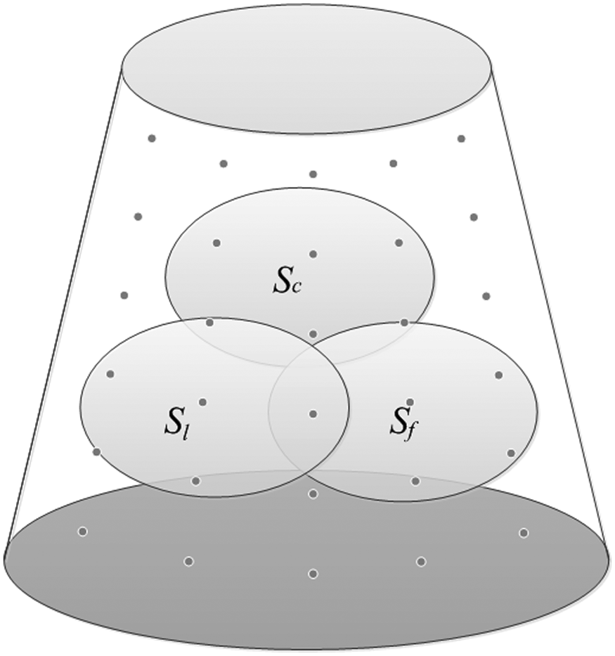
Different node sets by function.

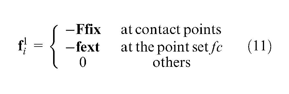
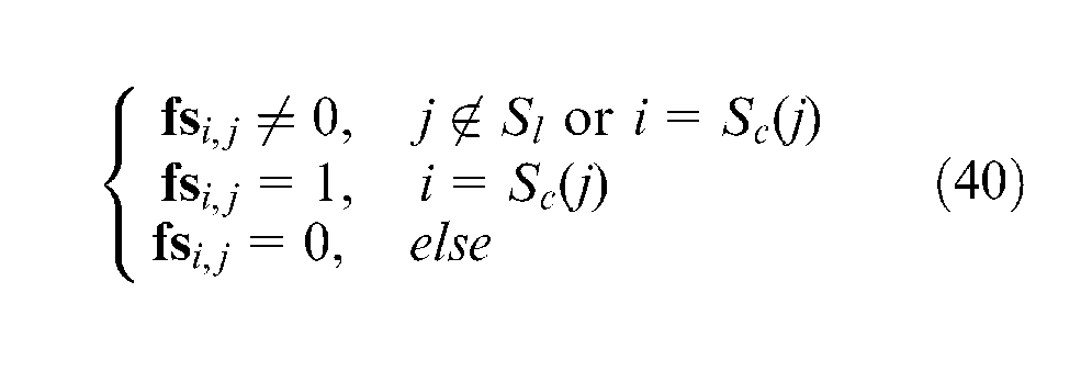
From equation (11), it can be seen that the reacting force of the workpiece is not equivalent to 0 only at the DOF of the contact point or $\mathrm{fc}$ . Additionally, both the DOF of the contact point and $\mathrm{fc}$ belong to the set of MDOF, so that the reacting force of the workpiece is equivalent to 0 except at the set of MDOF. Therefore, the reacting force ${\mathbf{f}}^1$ can be made with one linear space with the same order of MDOF. The basic idea of the accelerating method is to reduce the size of the stiffness matrix K and the solution vectors F · u into MDOF S, achieving one new matrix equation

$$\mathbf{K}\mathbf{\prime }\mathbf{u}\mathbf{\prime }=\mathbf{f}\mathbf{\prime }$$

(13)

One general method to accelerate the computing speed of an FEM equation is the cohesion method, and the basic process is given by

$$\begin{array}{c}\left[\begin{array}{cc}\hfill {\mathbf{K}}_{11}\hfill & \hfill {\mathbf{K}}_{12}\hfill \\ \multicolumn{1}{c}{{\mathbf{K}}_{21}}& \hfill {\mathbf{K}}_{22}\hfill \end{array}\right]\left[\begin{array}{c}\hfill {\mathbf{u}}_1\hfill \\ \multicolumn{1}{c}{{\mathbf{u}}_2}\end{array}\right]=\left[\begin{array}{c}\hfill {\mathbf{f}}_1\hfill \\ \multicolumn{1}{c}{{\mathbf{f}}_2}\end{array}\right]\hfill \\ \Rightarrow ({\mathbf{K}}_{11}-{\mathbf{K}}_{12}{\mathbf{K}}_{22}^{-1}{\mathbf{K}}_{21}){\mathbf{u}}_1={\mathbf{f}}_1-{\mathbf{K}}_{12}{\mathbf{K}}_{22}^{-1}{\mathbf{f}}_2\hfill \\ \Rightarrow \mathbf{K}\mathbf{\prime }\mathbf{u}\mathbf{\prime }=\mathbf{f}\mathbf{\prime }\hfill \end{array}$$

(14)

in which

$$\{\begin{array}{c}\hfill \mathbf{K}\mathbf{\prime }={\mathbf{K}}_{11}-{\mathbf{K}}_{12}{\mathbf{K}}_{22}^{-1}{\mathbf{K}}_{21}\hfill \\ \multicolumn{1}{c}{\mathbf{u}\mathbf{\prime }={\mathbf{u}}_1}\\ \multicolumn{1}{c}{\mathbf{f}\mathbf{\prime }={\mathbf{f}}_1-{\mathbf{K}}_{12}{\mathbf{K}}_{22}^{-1}\mathbf{f}}\end{array}$$

(15)

However, this approach requires too much additional computer memory, and there exists a gap between the limited computer resources and the complex workpiece model. In fact, all of the solutions of the FEM equation under different external forces in the MDOF set S are of one linear space, and the basic idea of every accelerating method is to construct the basis of the linear space. In this article, another method was constructed that requires less additional computer memory cost.

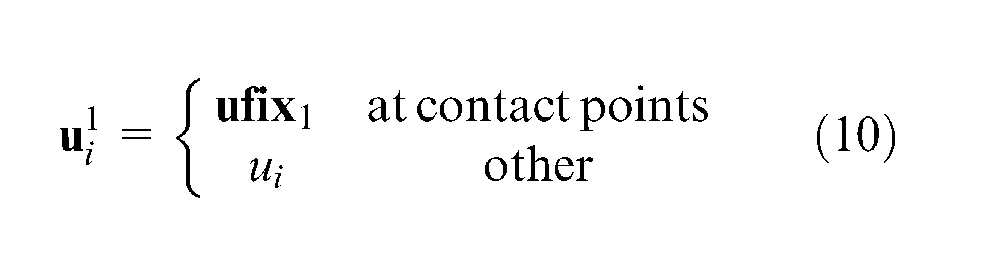
First, displacement constraints are acted at $S$ , given as

$$\begin{array}{l}\tilde{K}=K\\ \{\begin{array}{c}{\tilde{K}}_{i,:}=0\\ {\tilde{K}}_{:,i}=0\\ {\tilde{K}}_{i,i}=1\end{array}i\in S\\ {\widetilde{\mathit{\text{f}}}}_i=0i\in S\end{array}$$

(16)

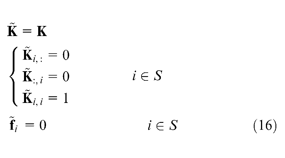
Then, unrestrict the freedom of $S$ stepwise, as

$$\{\begin{array}{c}\hfill {\tilde{\mathbf{K}}}_{j,:}={\mathbf{K}}_{j.:}\hfill \\ \multicolumn{1}{c}{{\tilde{\mathbf{K}}}_{:,j}={\mathbf{K}}_{:,j}}\\ \multicolumn{1}{c}{{\tilde{\mathbf{f}}}_j=1}\end{array}$$

(17)

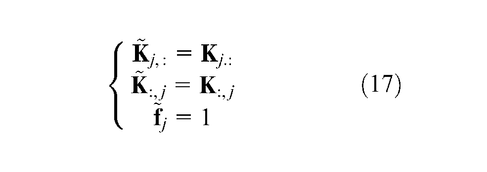
Solve the generated equations

$$\tilde{\mathbf{K}}{\mathbf{u}}_j={\tilde{\mathbf{f}}}_j$$

(18)

Next, the solutions of ${\mathbf{u}}_j$ and the related stress ${\mathbf{f}}_j$ can be easily obtained, although they must meet

$$\{\begin{array}{c}\hfill {\mathbf{f}}_j\ne 0,j\in S\hfill \\ \multicolumn{1}{c}{{\mathbf{f}}_j=0,\text{else}}\end{array}$$

(19)

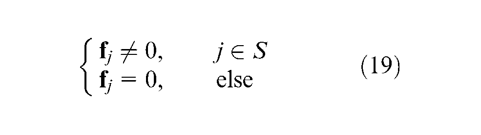
As shown in equation (19), non-zero stress only occurs at $S$ when one DOF of $S$ is deleted. Therefore, for all $S_j\in S$ , the solutions with linear operations can constitute two linear spaces, and the basis vectors of the two linear spaces are written as

$$\begin{array}{c}\mathbf{usub}=\{{\mathbf{u}}_{i,S}|i\in S\}\hfill \\ \mathbf{fsub}=\{{\mathbf{f}}_{i,S}|i\in S\}\hfill \end{array}$$

(20)

If a vector $\mathbf{\text{ε}}$ with the same size of $S$ is given, then

$${\mathbf{K}}_{S,:}\times u\epsilon =\mathbf{f}\mathbf{\text{ε}}$$

(21)

in which

$$\mathbf{u}\mathbf{\text{ε}}=\sum _{i\in S}{\mathbf{\text{ε}}}_i{\mathbf{u}}_i,\mathbf{f}\mathbf{\text{ε}}=\sum _{i\in S}{\mathbf{\text{ε}}}_i\mathbf{fsu}{\mathbf{b}}_{:,i}$$

(22)

Here ${\mathbf{K}}_{S,:}$ means the special rows of $\mathbf{K}$ within the MDOF set $S$ , while equation (18) is restricted by $S$ and changed to equation (21)

$$usub\epsilon =u{\epsilon }_S$$

(23)

in which

$$\mathbf{usu\; b}\epsilon ={\displaystyle \sum _{i\in S}{\mathbf{\epsilon }}_i\mathbf{usu}{\mathbf{b}}_i}$$

(24)

Furthermore, $u{\epsilon }_S$ denotes the components of $\mathbf{u}\mathbf{\epsilon }$ , of which the row number is limited to $S$ . The length of $\mathrm{usub}\epsilon$ is equal to $\mathbf{f}\mathbf{\text{ε}}$ and $S$ .

However, the solution of equation (12) suits equations (4), (5) and (15) and belongs to the linear space $\mathrm{usub}$ and $\mathbf{fsub}$ . According to the properties of the matrix function, every vector satisfied to one linear equation will be the same, which means if the constraints are the same, then the solution of equations (12) and (15)–(17) will be the same. Hence, after being given one constraint, then the related solution of $\mathbf{\epsilon }$ will be found by equations (16) and (17), and then $\mathbf{u}$ , $\mathbf{f}$ can be computed by equation (21). Thus, the basis of the linear space is constructed, and the solution of the contact model can be solved after the fixel model and the constraints are introduced into the linear space.

Finding the solution with the linear spaces

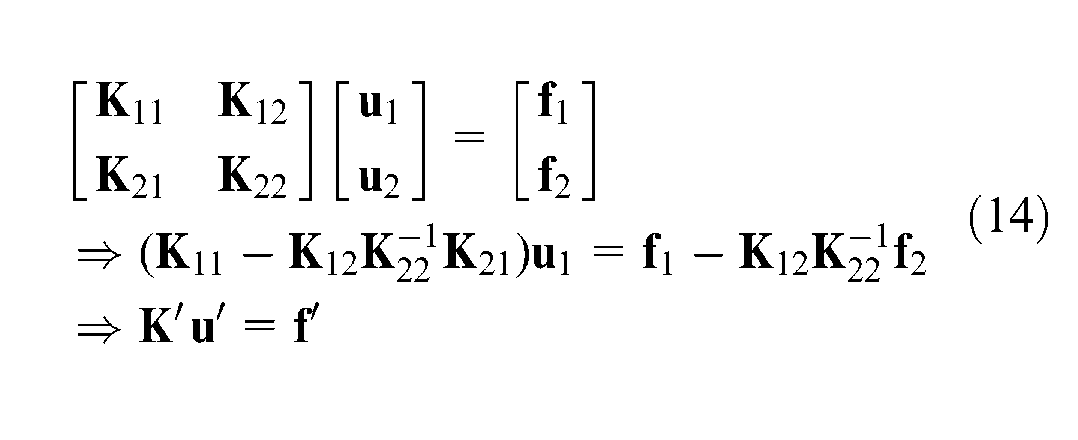
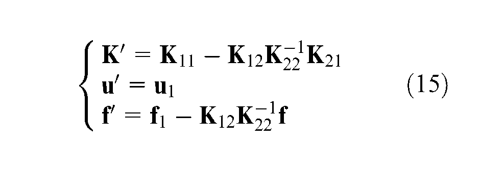
While the specific external force $\mathbf{fext}$ and the constraint $C,C\in S$ are given, the solution of $\mathbf{u}$ , $\mathbf{f}$ also must satisfy equations (3)–(6) and (21). Additionally, the related $\mathbf{\text{ε}}$ , $\mathbf{u}\mathbf{\text{ε}}$ , $\mathbf{f}\mathbf{\text{ε}}$ must satisfy equations (16) and (17).

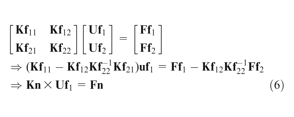
Due to equation (12), equation (9) can be rewritten as

$$\mathbf{Ffix}=\mathbf{Kfix}\times \mathbf{ufi}{\mathbf{x}}_1$$

(25)

This new equation (25) can be combined with equation (11), giving

$${\mathbf{f}}_i^1=-\mathbf{Ffix}=-\mathbf{Kfix}\times \mathbf{ufi}{\mathbf{x}}_1\text{at contact points}$$

(26)

As shown in equations (16) and (18), equation (26) can be rewritten in linear space

$$\mathbf{fsub}(C,:)\times \mathbf{\text{ε}}=-{\mathbf{K}}^{-1}\mathbf{usub}(C,:)\times \epsilon$$

(27)

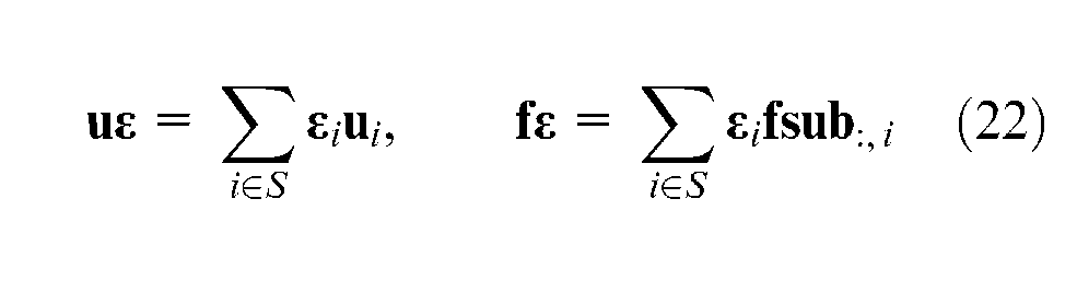
Additionally, the force vector must obey the external force. Based on these conditions, one method for constructing a linear equation to solve the vector $\mathbf{\epsilon }$ is given in equation (28)

$$\{\begin{array}{c}\hfill \mathbf{fsub}(C,:)\times \mathbf{\text{ε}}+{\mathbf{K}}^{-1}\mathbf{usub}(C,:)\times \mathbf{\text{ε}}=0\hfill \\ \multicolumn{1}{c}{\mathbf{fsub}(\mathrm{fc})\times \mathbf{\text{ε}}=-\mathbf{fext}}\end{array}$$

(28)

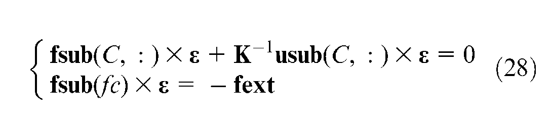
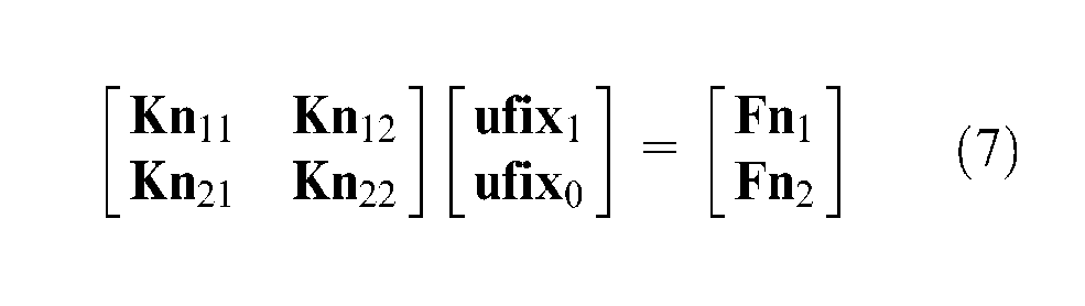
All three equations in equation (28) can be expressed by the two bases $\mathbf{usub},\mathbf{fsub}$ . The first equation of equation (28) indicates that the solution must be constrained at C, and the second denotes that the reacting force at $\mathrm{fc}$ must be equal to $\mathrm{fext}$ ; the last equation indicates that the reacting force at other freedoms must be 0.

After the matrix equation (28) is solved, the required $\epsilon$ can be obtained. Then, by the application of equations (6) and (15)–(17), the solution of $\mathbf{u},\mathbf{f}$ can be easily found. Hence, the computing problem of equation (12) is transformed into another computing problem, this time of equation (28). Equation (28) has the same order as $S$ , which is significantly less than that of equation (12), so the computing time cost of equation (28) is also significantly less than that of equation (12). As was shown before, the process of the accelerating method can be illustrated in Figure 2. Hence, the computing speed can be improved by reducing the freedom of the finite element (FE) matrix to a required size in accordance with this method.

Figure 2.

Accelerating method process.

Optimisation algorithm process of the fixture layout design

Constraints

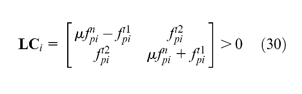
First, between the workpiece and the fixture, the contact force must obey the column friction rule and the normal component on the surface must be positive.

For one contact point $p_i$ , let the normal contact force be $f_{\mathrm{pi}}^n$ and the two orthogonal components of the frictional force be $f_{\mathrm{pi}}^{t1}$ and $f_{\mathrm{pi}}^{t2}$ ; then, the contact constraints can be written as

$$\{\begin{array}{c}\hfill f_{\mathrm{pi}}^n>0\hfill \\ \multicolumn{1}{c}{{\mu }^2{f}_{\mathrm{pi}}^{n2}>f_{\mathrm{pi}}^{t12}+f_{\mathrm{pi}}^{t22}}\end{array}$$

(29)

Inequality (equation (29)) is non-linear and thus will be difficult to compute or optimise; however, it can be transformed into

$$\mathbf{L}{\mathbf{C}}_i=\left[\begin{array}{cc}\hfill \mu f_{\mathrm{pi}}^n-f_{\mathrm{pi}}^{t1}\hfill & \hfill f_{\mathrm{pi}}^{t2}\hfill \\ \multicolumn{1}{c}{f_{\mathrm{pi}}^{t2}}& \hfill \mu f_{\mathrm{pi}}^n+f_{\mathrm{pi}}^{t1}\hfill \end{array}\right]>0$$

(30)

Next, it can be expanded to all contact points

$$\mathbf{LC}=\mathrm{diag}\{\mathbf{L}{\mathbf{C}}_1,\dots ,\mathbf{L}{\mathbf{C}}_i,\dots \}>0$$

(31)

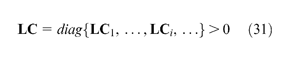
Then, inequality (equation (31)) is the contact constraint at all contact positions. Inequality (equation (31)) is of a typical LMI form, and the region defined by LMI is convex, which means that every convex or linear optimisation problem can be solved by some classical convex optimisation method. ¹⁷

Optimisation objective

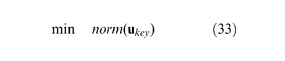
The machining accuracy is finally justified by the accuracy of the machining position; thus, one good fixture layout can significantly reduce the machining error of the machining position. The machining position can be divided into discrete points, and the displacement of these points can reflect the machining error caused by elastic deformation of the fixture–workpiece system. Due to this, the norm of the key-point displacement can be defined as the optimisation objective of the fixture layout design objective.

Let ${\mathbf{u}}_{\mathrm{key}}$ is the displacement vector of the key-points

$${\mathbf{u}}_{\mathrm{key}}=\mathbf{uk}(\mathrm{fixture}\_\mathrm{layout},\mathrm{clamping}\_\mathrm{force})$$

(32)

Then, the objective of the optimisation problem (equation (32)) can be defined as

$$min\mathrm{norm}({\mathbf{u}}_{\mathrm{key}})$$

(33)

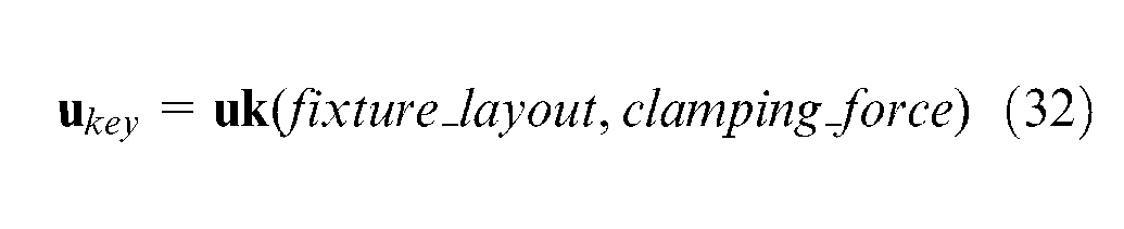
This objective function is a convex function. Additionally, the fixture layout and clamping force can be defined as

$$\begin{array}{c}\text{find}\mathrm{fixture}\_\mathrm{layout\; and\; clamping}\_\mathrm{force}\hfill \\ min\mathrm{norm}({\mathbf{u}}_{\mathrm{key}})\hfill \\ \mathrm{st}:\mathbf{LC}>0\hfill \end{array}$$

(34)

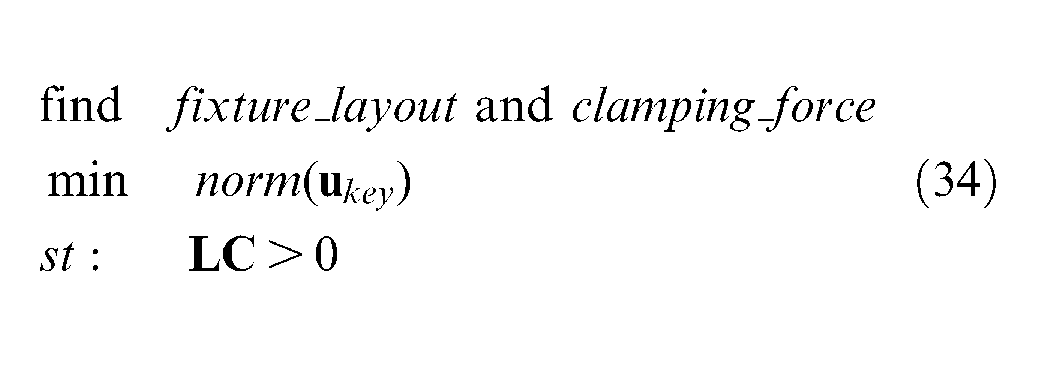
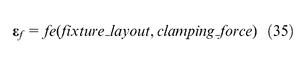
Both the fixture layout and the clamping force are important, and their relation to the fixing error ${\epsilon }_f$ can be written as

$${\mathbf{\text{ε}}}_f=\mathrm{fe}(\mathrm{fixture}\_\mathrm{layout},\mathrm{clamping}\_\mathrm{force})$$

(35)

However, there exists one group of clamping forces with which a minimum fixing error can be reached once the special fixture layout fl₁ and the external force are given. Furthermore, the clamping force can be called the optimal force, meaning that the clamping force can be obtained by solving the optimisation problem (equation (36))

$$\begin{array}{c}\mathrm{find}\mathrm{clamping}\_\mathrm{force}\hfill \\ min\mathrm{norm}({\mathbf{u}}_{\mathrm{key}})\hfill \\ \mathrm{st}:\mathbf{LC}>0\hfill \end{array}$$

(36)

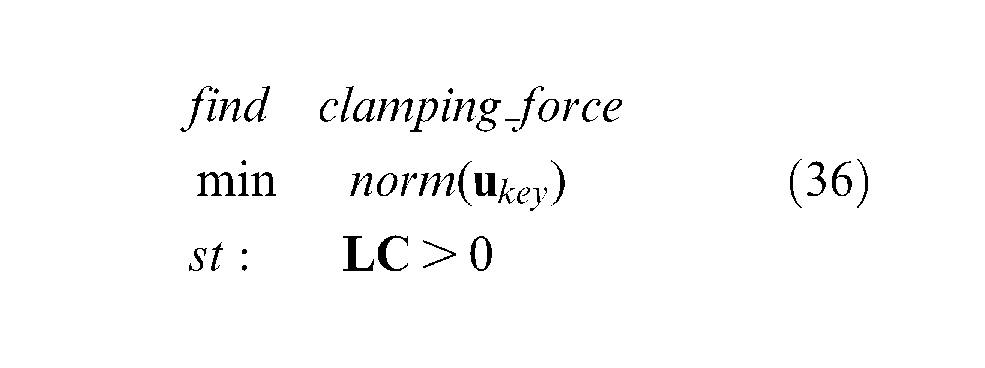
in which ${\mathbf{u}}_{\mathrm{key}}$ is a function of the clamping force

$${\mathbf{u}}_{\mathrm{key}}=\mathbf{uk}(f{l}_1,\mathrm{clamping}\_\mathrm{force})=\mathbf{u}{\mathbf{k}}_0(\mathrm{clamping}\_\mathrm{force})$$

(37)

Under a fixed external force, the clamping force can be written as a function of the fixture layout

$$\mathrm{clamping}\_\mathrm{force}=\mathrm{cf}(\mathrm{fixture}\_\mathrm{layout})$$

(38)

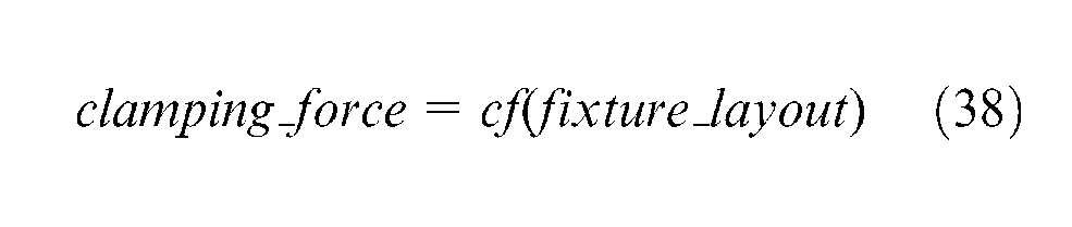
The function cf denotes that the optimisation result of the solved optimisation problem is a special optimisation method.

Then, equation (35) can be rewritten as

$$\begin{array}{l}{\epsilon }_f=\mathrm{fe}(\mathrm{fixture}\_\mathrm{layout},cf(\mathrm{fixture}\_\mathrm{layout}))\\ =\mathrm{ge}(\mathrm{fixture}\_\mathrm{layout})\end{array}$$

(39)

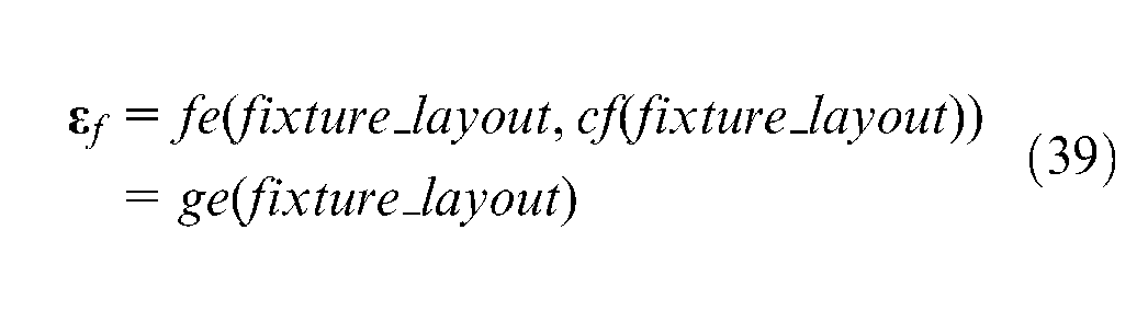
Hence, it can be found that the force optimisation is a sub-problem of the fixture layout optimisation.

Clamping force optimisation method

Most FEM-based clamping force optimisation methods are time expensive due to the frequent calling of FEM computing. Hence, the key issue in embedding the force optimisation into the fixture layout optimisation process is the reduction of the time cost.

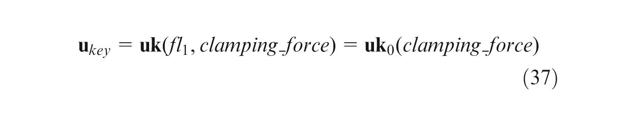
Given one group of fixture layouts, then the displacement constraint and external force are fixed, and only the clamping force is an undetermined parameter. Furthermore, the clamping force can only be acted on by the freedom in $S_c$ . This can be seen as a special case of the problem discussed in section ‘Accelerating solving method of the contact model’, in which the contact points are fixed and the clamping force is variable. Similarly, when the deformation and the stress vector are under different forces, the deformation and the stress vector are also of one linear space. Based on this, the basis vector $\mathbf{fs}$ of the linear space $\mathbf{Fs}$ can be defined as

$$\{\begin{array}{c}\hfill \begin{array}{c}\hfill \mathbf{f}{\mathbf{s}}_{i,j}\ne 0,j\notin S_l\text{or}i=S_c(j)\hfill \\ \multicolumn{1}{c}{\mathbf{f}{\mathbf{s}}_{i,j}=1,i=S_c(j)}\end{array}\hfill \\ \multicolumn{1}{c}{\mathbf{f}{\mathbf{s}}_{i,j}=0,\mathrm{else}}\end{array}$$

(40)

Furthermore, all stress vectors generated by the possible clamping force must belong to the above space, meaning that there must be one $\mathbf{fc}$ for a given $\mathbf{f}$ , which suits

$$\mathbf{f}\mathbf{=}\mathbf{fs}\times \mathbf{fc}$$

(41)

Then, clamping position $\mathbf{f}$ must meet

$$\mathbf{f}\mathbf{=}\mathbf{fc}$$

(42)

This means that $\mathbf{fc}$ receives the same value of clamping_force.

According to the uniqueness theorems of the solutions for linear equations, $\mathbf{f}$ must be the stress vector under one group of clamping forces equal to $\mathbf{fc}$ . Additionally, the corresponding displacement $\mathbf{u}$ can be reached by equation (1).

Hence, the stress and the displacement vector can be written as linear functions of the clamping force under the special fixture layout. This means that the function ${\mathbf{u}}_{\mathrm{key}}$ is linear. Hence, the optimisation problem (equation (39)) can be rewritten as

$$\begin{array}{c}\mathrm{find}\mathbf{fc}\hfill \\ min\mathrm{norm}({\mathbf{u}}_{\mathrm{key}})\hfill \\ \mathrm{st}:\mathbf{f}\mathbf{=}\mathbf{fs}·\mathbf{fc}\hfill \\ \mathbf{LC}>0\hfill \end{array}$$

(43)

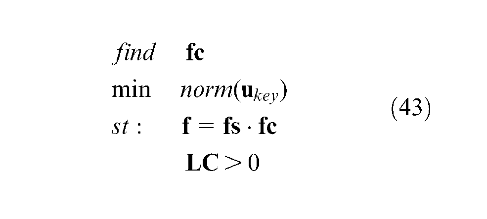
Furthermore, it is a typical convex optimisation within the norm of LMI and can be solved quickly with very few FEM computational callings.

Integral fixture layout optimisation method

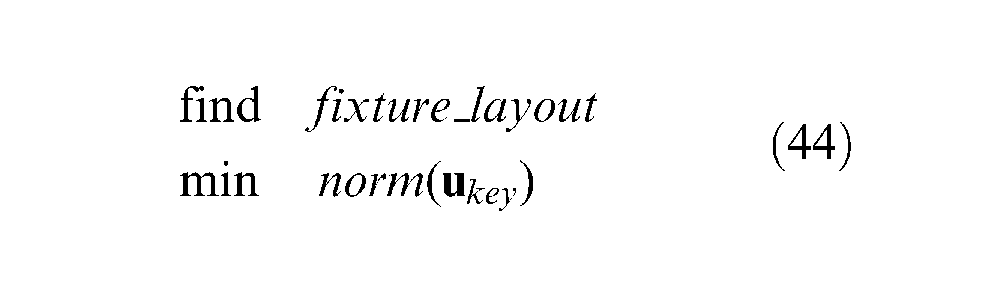
Because the clamping force can be optimised by solving the optimisation problem (equation (43)), and the optimal result can be defined by function (38), the design variations of the optimisation problem (equation (34)) can be reduced to {fixture_layout}. Meanwhile, the constraint of the optimisation problem is considered in the force optimisation process, so the optimisation problem (equation (34)) can be simplified to

$$\begin{array}{c}\text{find}\mathrm{fixture}\_\mathrm{layout}\hfill \\ min\mathrm{norm}({\mathbf{u}}_{\mathrm{key}})\hfill \end{array}$$

(44)

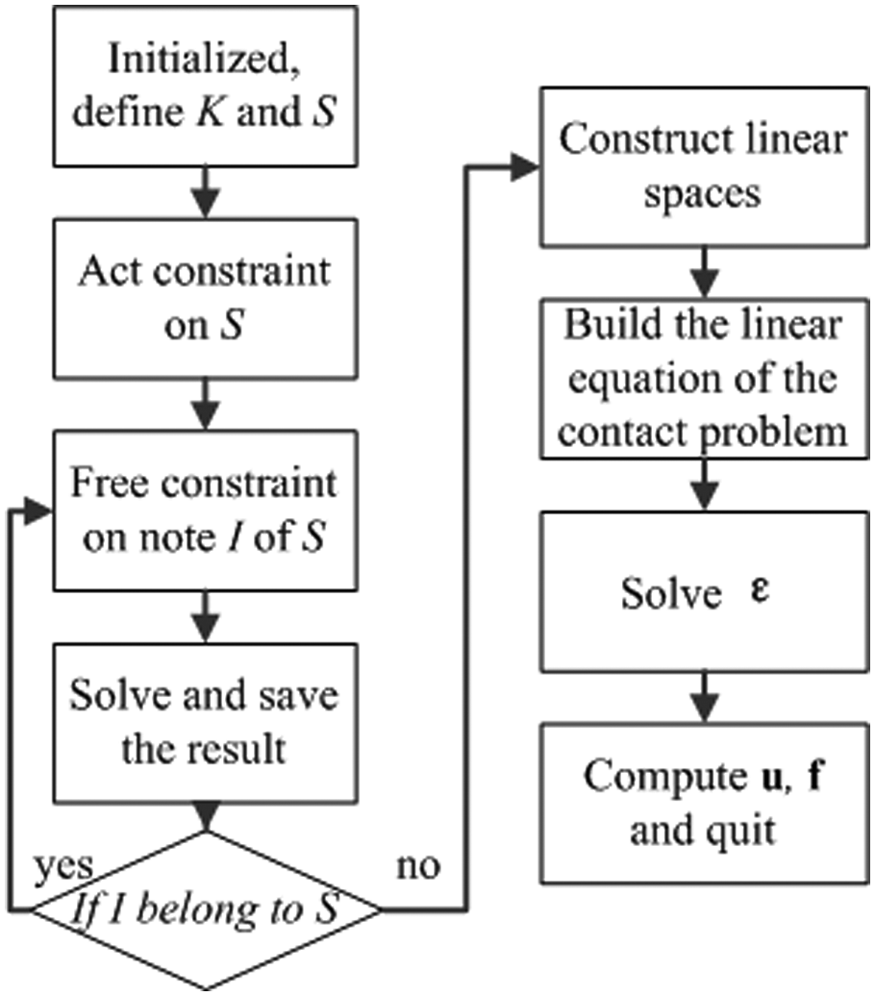
Combined with the typical GA method, an integral optimisation method of the fixture layout design is constructed, and its flowchart is shown in Figure 3:

• Step 1. As shown in Figure 3, before commencing the design of the fixture layout, the computer-aided design (CAD) model of the workpiece must be given.

• Step 2. Then, the CAD model can be modelled to obtain the mesh and the nodes, and the nodes should be numbered.

• Step 3. The FEM equation together with the stiffness can be generated in sequence.

• Step 4. The FEM equation can be operated as the proposed accelerating method.

• Step 5. Then, the FEM equation can be initialised and the initial fixture layout can be obtained.

• Step 6. The optimal clamping force of the special fixture layout can be solved.

• Step 7. Followed by computation of the displacement vector of the key-points under the optimal clamping force.

• Step 8. Finally, steps 5–7 should be iterated by the GA process to yield one optimal fixture layout. End.

Figure 3.

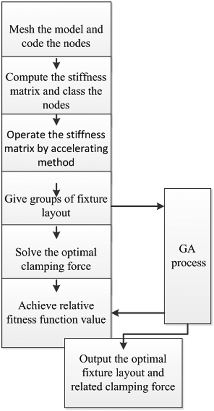
Flowchart of the optimisation design method of the fixture layout and the clamping force.

A numerical example

Example A: operating a simple workpiece

To show the performance of the accelerated method, a simple workpiece is taken into practice, and it is shown in Figure 4.

Figure 4.

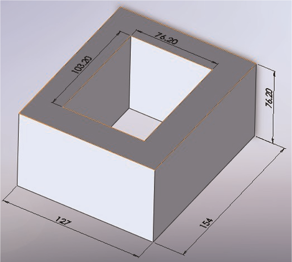
Geometric features of the workpiece (units: mm).

• Computer resource:

•  CPU: Pentium E5300 2.6 GHz

•  Memory: 2 GB

After the workpiece is meshed, a stiffness matrix measuring 4590 × 4590 is obtained. Operating the stiffness matrix according to Figure 2, its size is decreased to 1440 × 1440. Figure 5 shows the additional memory cost of our method in comparison to that of the cohesion method. As a result of the operating process, the time cost of the FEM equation solving is reduced from approximately 4 s to less than 1 s.

Figure 5.

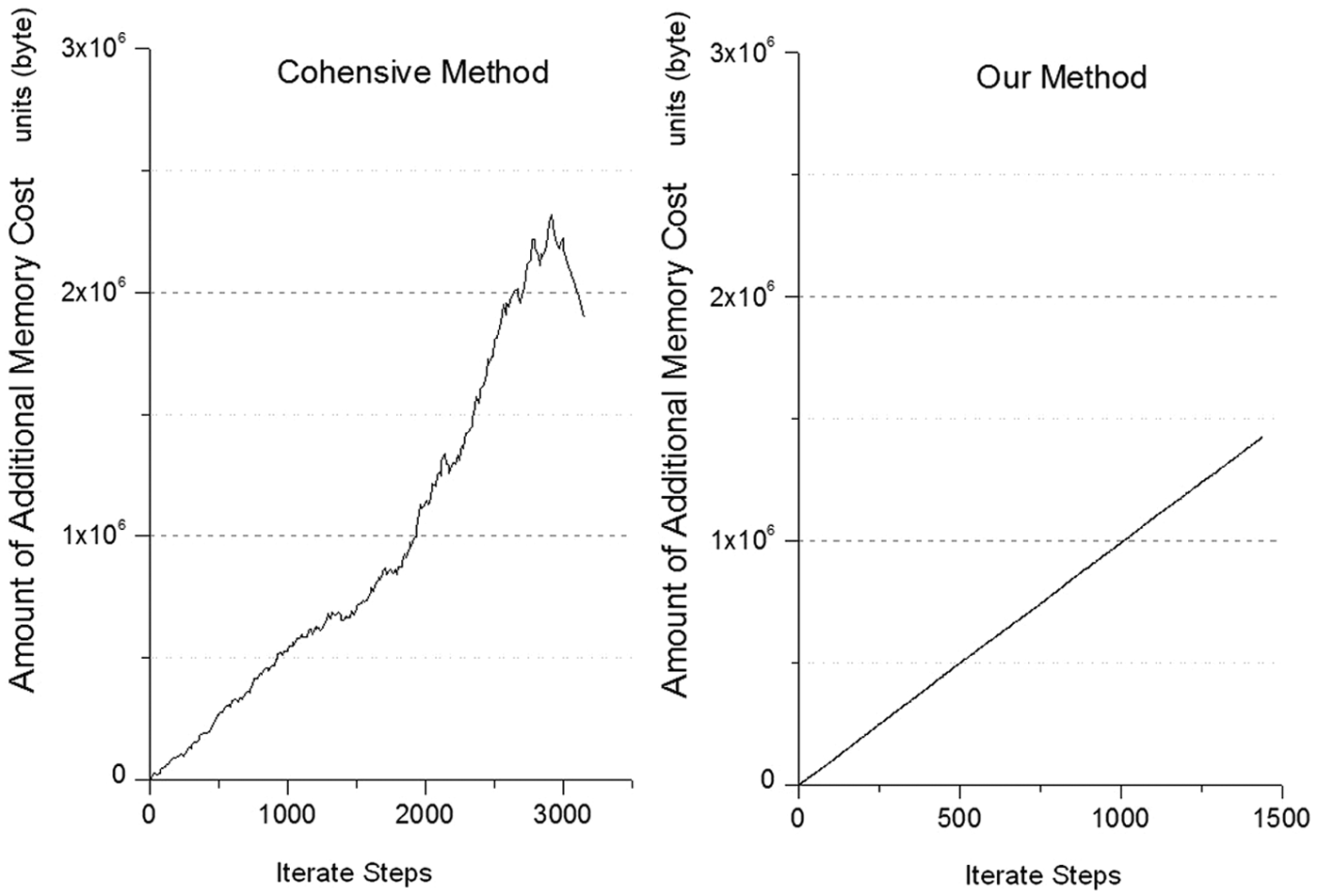
Additional memory cost.

In Figure 5, the x-axis is the iterative step of the accelerating method, and the y-axis is the amount of the additional memory cost. First, the ending values of the x-axis are different: in the left image, the x-axis ends at more than 3000, while in the right image, it is less than 1500. This is because the iterative step amount is equal to the order of the matrix equation minus the size of MDOF. Second, the memory cost of our method is increased as the iterating step is carried out. Third, there is a peak in the left image, which means each run of the cohesion method requires the greatest additional memory cost as that of the peak, which is significantly bigger than the cost associated with our method.

In our method, if the MDOF is a and the DOF of the original FEM matrix is b, then as is written above, the iterating step number of our method is a, while the cohesion method requires b–a iterating steps. This means that the memory cost of our method decreases as the value of a gets smaller. Additionally, because our method achieves an iterating step number of a, the speed is faster when the value of a is smaller. Furthermore, the computing speed of an individual matrix function is mainly influenced by its size; thus, the computing speed of the operated matrix function will be faster once the value of a is decreased.

We can conclude the following:

1. Our method requires less additional memory than the cohesion method.

2. As the MDOF is reduced, both the iterating time and the additional memory required are also reduced in our method.

3. As the MDOF is reduced, both the iterating time and the computing time required are also reduced in our method.

Example B: fixture layout and clamping force optimisation

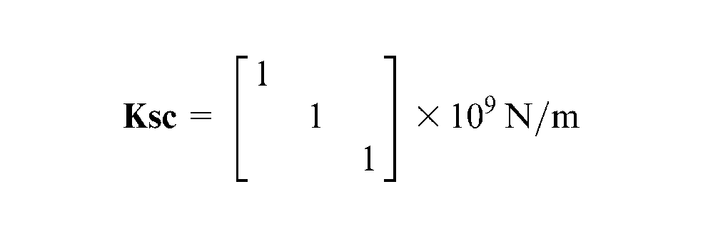
Figure 6 is the mesh of a blade model, and based on this mesh, a single stiffness matrix is obtained. The matrix has a size of 20265 × 20265, and then, it is operated on by the accelerating method with MDOF of 1830. The calculating time of the FEM balance equation is decreased from approximately 8–1.5 s. The fixels are assumed to be springs, which have a stiffness matrix of

$$\mathbf{Ksc}=\left[\begin{array}{ccc}\hfill 1\hfill & \hfill \hfill & \hfill \hfill \\ \multicolumn{1}{c}{}& \hfill 1\hfill & \hfill \hfill \\ \multicolumn{1}{c}{}& \hfill \hfill & \hfill 1\hfill \end{array}\right]\times {10}^9\text{N}/\text{m}$$

Figure 6.

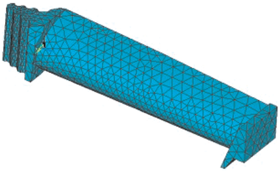
Mesh of the blade model.

In each iterating step, one clamping force must be called. Then, the fixture layout and the clamping force optimisation program are built, and one clamping force must be called in every iterating step. One running history of the clamping force optimisation is shown in Figure 7. This problem clearly only requires a few steps to converge to the final result.

Figure 7.

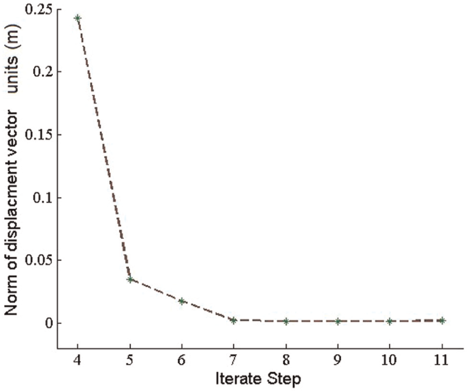
Convergence history of the clamping force optimisation.

In every run, the linear space basis of the resulting vector must be calculated first under the given fixture layout, which requires three times that of the FEM computing load. Next, the convex optimal method is run in the smaller linear space. The computing time of each iteration is far less than the original FEM computing time, and only a small number of iterations are needed. In this example, three times the FEM computing cost is approximately 5 s, while the total time of the convex method is less than 2 s. Therefore, the clamping force optimisation method is fast enough that it can be used in every iteration of the fixture layout optimisation process.

With the aim to obtain six locators around the convex surface and three clampers on the concave surface, one optimisation algorithm is constructed. After the optimisation program runs, one optimal fixture layout and the related clamping force are developed. The iterating process and the optimal layout are shown in Figures 8 and 9, in which Figure 9(a) shows the locator positions and Figure 9(b) shows the result of the clampers.

Figure 8.

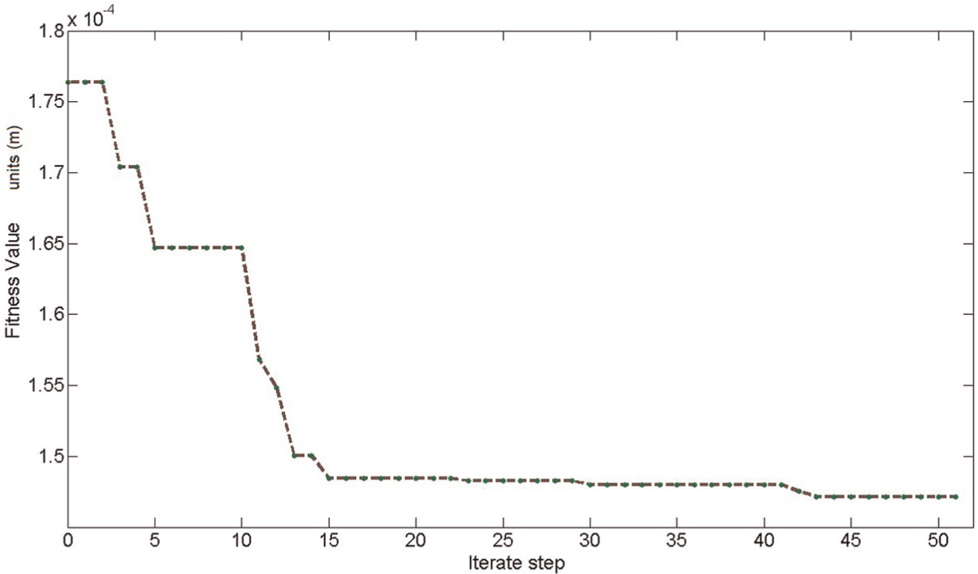
Convergence history of the fixture layout optimisation.

Figure 9.

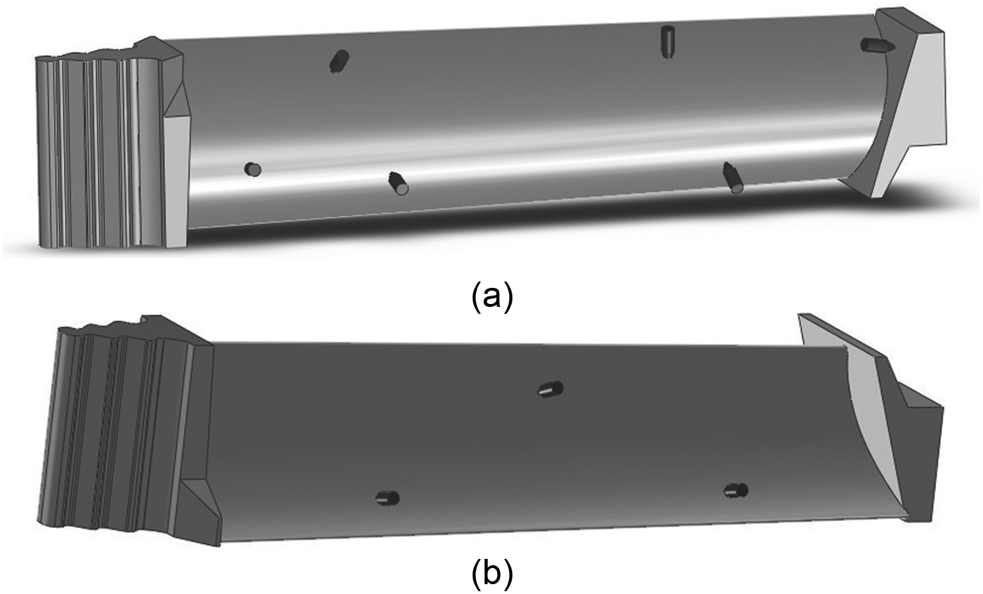
Final result of the fixture layout: (a) final result of the locator positions and (b) final result of the clamper positions.

Conclusion

In this article, a highly efficient, accelerated fixture layout and clamping force optimisation method are presented with the goal to reduce the elastic deformation of the workpiece–fixture system:

1. Initially, the FEM model was built to illustrate the contact problem. To improve the time cost, one method is presented to accelerate the speed of solving the FEM equation. This method can be used in both the elastic–rigid contact problem and the elastic–elastic contact problem for the workpiece–fixture system. Additionally, it was demonstrated that these problems can be solved with low memory cost, and the memory cost can be decreased as the MDOF is shortened. Given examples were used to illustrate the performance of the method.

   More than these, for the accelerating method can be used to combine the stiffness matrix of fixels, it can be used for any non-linear workpiece–fixture contact model based on FEM as well. As one application of this method, we have built one non-linear contact model for workpiece–fixture system considering fixel’s geometry and more complex contact status between workpiece and fixture, which will be presented later. The accelerating method can be used for the optimisation issue of complex systems with such a big memory and computing time as the fixture layout optimisation problem presented here.

2. Furthermore, this idea can be used to study clamping force optimisation. Combined with an LMI description of the column friction constraint, the clamping force optimisation was modelled as a typical convex optimisation method in a linear space, achieving comparatively fast solution times. This clamping force optimisation method requires very few calling times during the FEM process, and the time cost of the clamping force optimisation process is minimal, so that it can be planted in the fixture layout optimisation.

3. Based on the above results and the GA method, an integral optimisation method for the fixture layout was built. To show its convergence, a related example was introduced to plan the fixture layout of a complex blade.