
Abstract
Laser shearography is a relatively new and useful method for nondestructive testing of many kinds of material that need robust methods to be applicable in industrial environments. To get the best results of this inspection method, adjusting the loading parameters properly and precisely is of a great consideration. In this article, a new numerical–experimental procedure to study the effects of thermal loading parameters in the shearography test of defected materials is presented. In this regard, a numerical procedure was developed to simulate shearographic fringe patterns using finite element analysis and supplementary programming. The modeling method was evaluated using experimental tests in a Plexiglas circle subjected to the thermal and mechanical loadings. Flat-bottom holes indicating internal defects of the test part were simulated and experimented to study the parameters that should be adjusted and controlled to get desirable outcomes from shearography nondestructive testing. It has been showed that for each distinct case of nondestructive testing, a thermal loading diagram can be extracted to get credible results.
Keywords
Introduction
Recent advances in material development have resulted in a wide range of novel nondestructive testing (NDT) techniques because many traditional techniques have not been capable of providing reliable, quantitative information regarding the state of damage and overall integrity in such materials.
Among the various new NDT techniques, optical ones are emerging as strong tools, because of their nature of being full-field, noncontacting, and noncontaminating. 1 Moreover, the results of the inspection of optical methods are images that give visual representations of the condition of the components. 2 Optical methods of NDT include thermography, 3 holography, 4 Moiré interferometry, 5 electronic speckle pattern interferometry (ESPI), 6 and shearography. 7
Shearography (as called speckle pattern shearing interferometry) was first introduced as a full-field strain analysis technique by Hung and Taylor. 8 In shearography, there is no more need for the reference beam of holography and, consequently, no more need to vibration isolation compared to other coherent optical techniques. In addition, since shearography measures displacement derivatives directly, it is insensitive to rigid-body motions that often produce misleading results in both holographic interferometry and ESPI. 9 These advantages have rendered shearography a potentially valuable tool for industrial NDT. This method offers optimal conditions for the direct measurement of strain information in the surface of the object. Because flaws usually generate strain concentration, shearography reveals a defect within an object by identifying defect-induced strain anomalies. Flaws in a material will give rise to strain concentrations when the object is loaded, and the strain concentrations form a fringe pattern that is used to detect and analyze the flaws. 10 The key to the success of shearography in defect detection is to impose an appropriate stress status on the object under investigation. The most common excitation methods to reveal defects are pressurizing, partial vacuum, mechanical loading, thermal excitation, and excitation by vibration.
Many industries interest shearography as an effective nondestructive evaluating technique. For example, rubber industry routinely uses shearography for evaluating tires, and the aerospace industry has adopted it for NDT of aircraft, in particular, composite structures. 11
Many researchers have studied shearography as a full-field strain measurement and NDT technique and investigated its parameters and applications. A review of shearography and its application for testing of composite structures has been presented by Hung. 12 Nokes and Cloud 13 used shearography and ESPI to detect internal damages excited by thermal and mechanical loadings in graphite–epoxy composites, which were damaged by milling a blind hole in the center of the panel. However, neither technique provided a definitive location of the flaw. Sirohi et al. 14 applied digital shearography to the NDT of plate structures by developing a procedure to measure the thickness of the plate. A theoretical relationship between the curvature of the surface of the defect and its thickness was obtained and verified experimentally.
In the recent studies, Zhanwei et al. 15 investigate the capabilities of shearography for detecting hole- and crack-type defects in polymer and metallic materials using thermal loading, and DeAngelis et al. 16 used vibration dynamic loading to reveal flat-bottom holes made with different sizes and placed at different depths in carbon fiber–reinforced plastic (CFRP) laminates. They evaluated the flaw detection capabilities of shearography by measuring dynamic response of defects to applied stresses by a proposed numerical–experimental procedure.
In this article, a new numerical–experimental approach to shearography is performed to investigate the defects excited by thermal loading in polymer materials. In this purpose, shearography fringe patterns of test specimens subjected to the thermal and mechanical loadings have been modeled using finite element method (FEM) and experimentally evaluated to confirm modeling procedure. Since all the known finite element (FE) packages do not deliver contours of out-of-plane displacement derivatives directly, an appropriate program has been developed to display the desired contours from the FEM outputs. A coupled thermoelastic analysis is performed to indicate the out-of-plane displacements created by thermal loading, and displacement derivatives have then been extracted by means of developed program.
Flat-bottom holes, indicating internal defects of specimens, 16 have then been made in the test plate with different sizes and depths. By comparison of FEM and experimental results, a loading factor is extracted to justify the FE analysis. Based on the confirmed models and experimental data, the comprehensive study of thermal loading parameters has been conducted.
Principles of shearography
Shearography is a full-field speckle interferometry technique that is sensitive to displacement gradient. The test object is illuminated by an expanded laser beam forming a speckle image. The main principle of the shearography is to make a pair of identical but laterally displaced, or sheared, speckle images. These two sheared images interfere in the imaging surface of a charged coupled device (CCD) camera to form a speckle interferogram that can be recorded and stored in a computer. After the object is stressed, the second speckle pattern is registered by the CCD camera again and stored in another frame. Digital subtraction between these two recorded images forms a fringe pattern depicting surface strain or displacement gradient distribution.
There are many devices that make a laterally sheared image in a shearography setup like: wedge plate, 17 Savart’s polariscope, 18 Wollaston’s prism, 19 wedge prism, 20 and modified Michelson-based interferometer. 9 A typical optical setup of digital shearography based on the modified Michelson interferometer is shown in Figure 1.
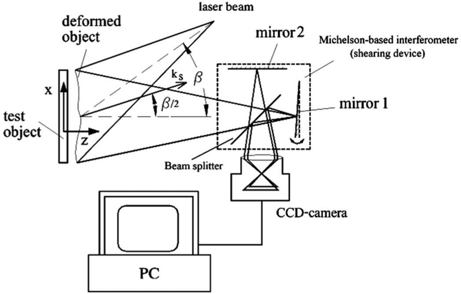
A typical setup of digital shearography based on the Michelson interferometer
The Michelson interferometer consists of a beam splitter and two orthogonally placed mirrors on two sides of the beam splitter. When the light reflects from the surface of the object, it is focused on the image plane of the CCD camera via these two mirrors. By turning mirror 1 or 2 for a very small angle, a pair of laterally sheared images of the test object is generated on the CCD camera. The two sheared images interfere with each other producing a speckle pattern. The amount of the shearing distance can be easily adjusted by turning one of the mirrors in the Michelson interferometer.
The intensity distribution

where I0 represents the average intensity of the two sheared light waves, γ represents the modulation of the interference term, and

where
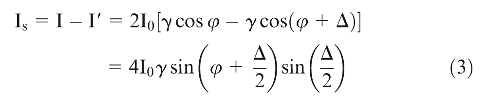
The result of the subtraction operation between the two digitized intensity distributions yields a fringe pattern indicated by equation (3) that can be displayed on the monitor in real time (at video rate). From equation (3), it is concluded that if Δ = 2πN, where N is an integer, dark fringes are formed, and brightness is a maximum when the relative phase change is equal to (2N + 1). In this manner, dark and bright fringes can be sequentially numbered with integers.
It can be shown7,9,10 that the relative phase change is related to the displacement derivatives instead of displacement itself due to the shearing function of shearography.
According to Figure 1,
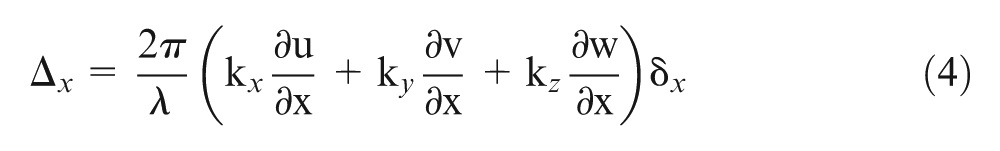
where δ x is the amount of shear directed along the x-axis; λ is the illuminating light wavelength; and u, v, and w are the displacement components along the references x-, y- and z-axes, respectively. In the case where the shearing direction lies in the y-axis, equation (4) becomes
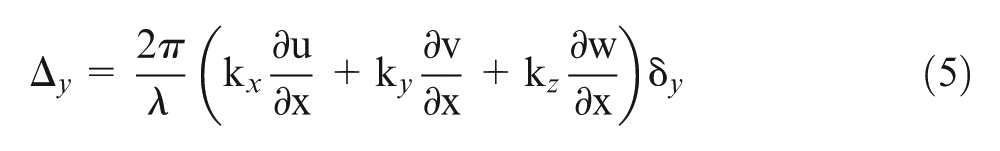
where δ y is the amount of shear along the y-axis.
If the observation and illumination positions lie in the x and z planes and the region of the object that is imaged by the camera is small compared to the source-to-object and object-to-camera distances, then the phase difference can be represented by
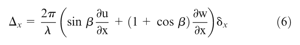
where β is the angle between the illumination and observation directions.
By making the observation and illumination directions close to collinear, the term sin β in equation (6) would be very small, and then the system would become sensitive only to the out-of-plane displacement gradient component. In this case, equation (6) reduces to
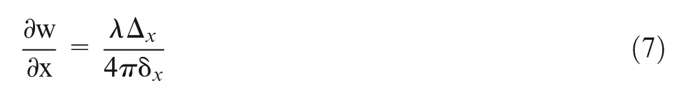
And for shear in y direction
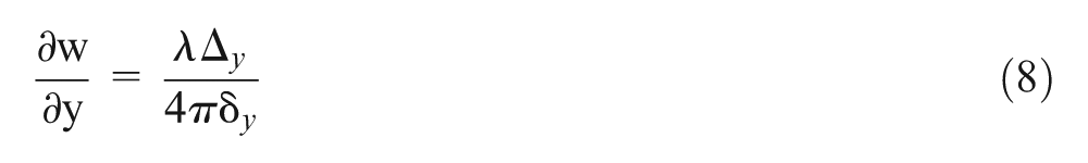
Hence, the out-of-plane components
As it is mentioned before, to make shearograms from a test part, it should be subjected to a kind of loading. This article is focused on the thermal loading, applied to the external surface of the object under test.
FE simulation of shearograms
FEM is used to simulate shearograms of test specimens, subjected to thermal loading. To evaluate the modeling method and adjusting parameters, a thin circular plate, clamped through its edge, was modeled and tested with a proper shearography setup. By comparing the results of the experiments and FE simulation, the modeling procedure can be approved.
FEM simulation
A fully clamped 100-mm-diameter circular plate with a thickness of 1.5 mm is simulated using the FE simulation. The temperature fields and the evolution of the out-of plane displacement due to the thermal loading are investigated. In this study, the thermoelastic behavior of the plate during heating and cooling is simulated using uncoupled formulation. This means that the heat conduction problem is solved independently from the displacement problem to obtain temperature history. However, the formulation considers the contributions of the transient temperature field to the mechanical analysis through the thermal expansion, as well as thermophysical and mechanical properties.
The governing equation of the transient heat transfer during heating and cooling processes is given by 22
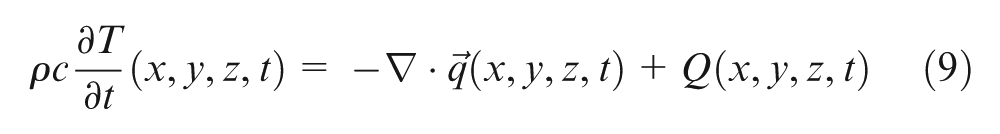
where T, t,

where
In the transient thermal analysis, the heating load is applied to the model, as “nodal temperature” as it can be measured directly in the experiments. The method of applying the surface temperature is considered to be “ramp loading” that means increasing the surface temperature, continuously and linearly, from the ambient temperature to the maximum measured temperature during the heating time. In the mechanical analysis, the temperature history obtained from the thermal analysis is inputted into the model as a thermal loading. Thermal strains and displacements are then calculated at each time increment. Thermal analysis was performed during both heating up and cooling down to calculate the temperature history. On the other hand, the resulted thermal strain takes place in the elastic region due to very low thermal loading. So, the thermal strains can be calculated in any time just by applying the temperature information of all of the nodes in the FE analysis.
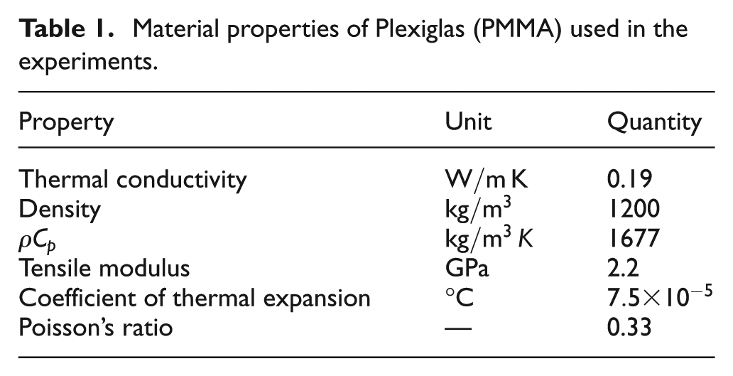
The material of the test plate investigated in this study is Plexiglas (polymethyl methacrylate (PMMA)), which is produced by casting, and its thermal and mechanical properties are entered in the FEM analysis according to Table 1. Because the thermal loading in this study does not exceed 60 °C, the dependency of properties to the temperature is neglected. Note that the maximum temperature of the sample test surfaces was measured using an infrared thermometer with an accuracy of ±1%.
Material properties of Plexiglas (PMMA) used in the experiments.
The applied thermal boundary conditions include the convection to the environment from all sides of the plate, the heat transfer coefficient is considered to be 5 W/m2 K as for free convection. In the mechanical analysis, the circle is fully clamped all around, as shown schematically in Figure 2. After the model is run, the out-of-plane displacement field is extracted for each time increment of the mechanical analysis while cooling down the specimen. Mechanical loading is also modeled in the FE analysis by applying a 10 µm displacement to the plate center.
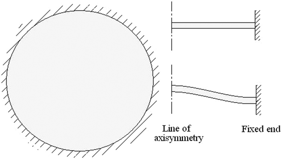
Mechanical boundary condition of the model in the FE analysis.
All analyses are performed using the FE analysis software ANSYS
23
but since all the known FE packages do not deliver desired contours of displacement derivatives directly, an appropriate program has been developed to display the desired contours of
Experiment
In this step, an out-of-plane shearography setup was generated according to Figure 1 using optical elements, a 3.2-megapixel digital CCD camera and 30 mW He–Ne laser (wavelength λ = 632.8 nm). A 100-mm-diameter circular plate, made from Plexiglas with a thickness of 1.5 mm, is fully clamped in its edge by means of a prepared fixture, as shown in Figure 3(a). The amount of shear distance is adjusted to 5 mm in x direction (δx = 5 mm). Mechanical and thermal loadings were applied to the test plate, and fringe patterns of the shearography were obtained by the proposed setup.
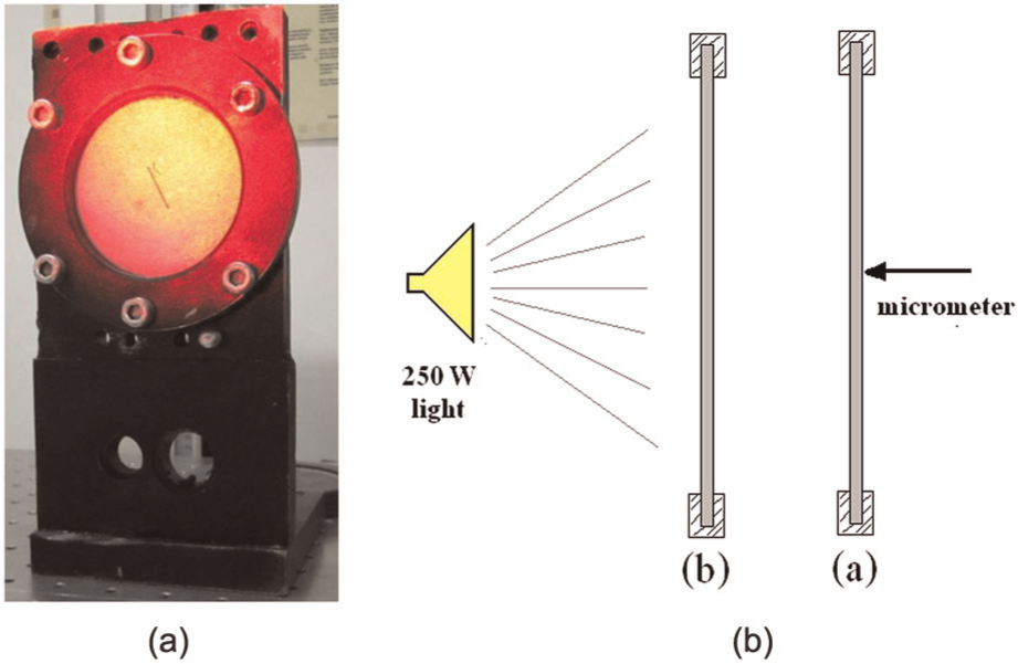
Prepared clamping fixture and loading schemas: (a) clamping fixture and (b) thermal and mechanical loadings of the specimen.
In the mechanical loading, the center of the plate was loaded by means of a fine micrometer to 10 µm (Figure 3(b)). Thermal loading was conducted using a 250-W thermal light adjusted in front of the test plate (Figure 3(b)). The light was glinted for 3 s. As mentioned before, experiments show that during the heating up phase, the surface temperature reaches almost 60 °C. Specklegrams were taken every 2 s while cooling down the specimen because the reflected light caused by the heating light prevents taking specklegram photos from the surface during heating up. Moreover, the heating time is very short, and taking several images in distinct times is not precise.
Resultant shearographic correlation fringe patterns, wrapped and unwrapped phase maps, and relevant contours of FEM analysis for mechanical and thermal loadings are shown in Figures 4 and 5.
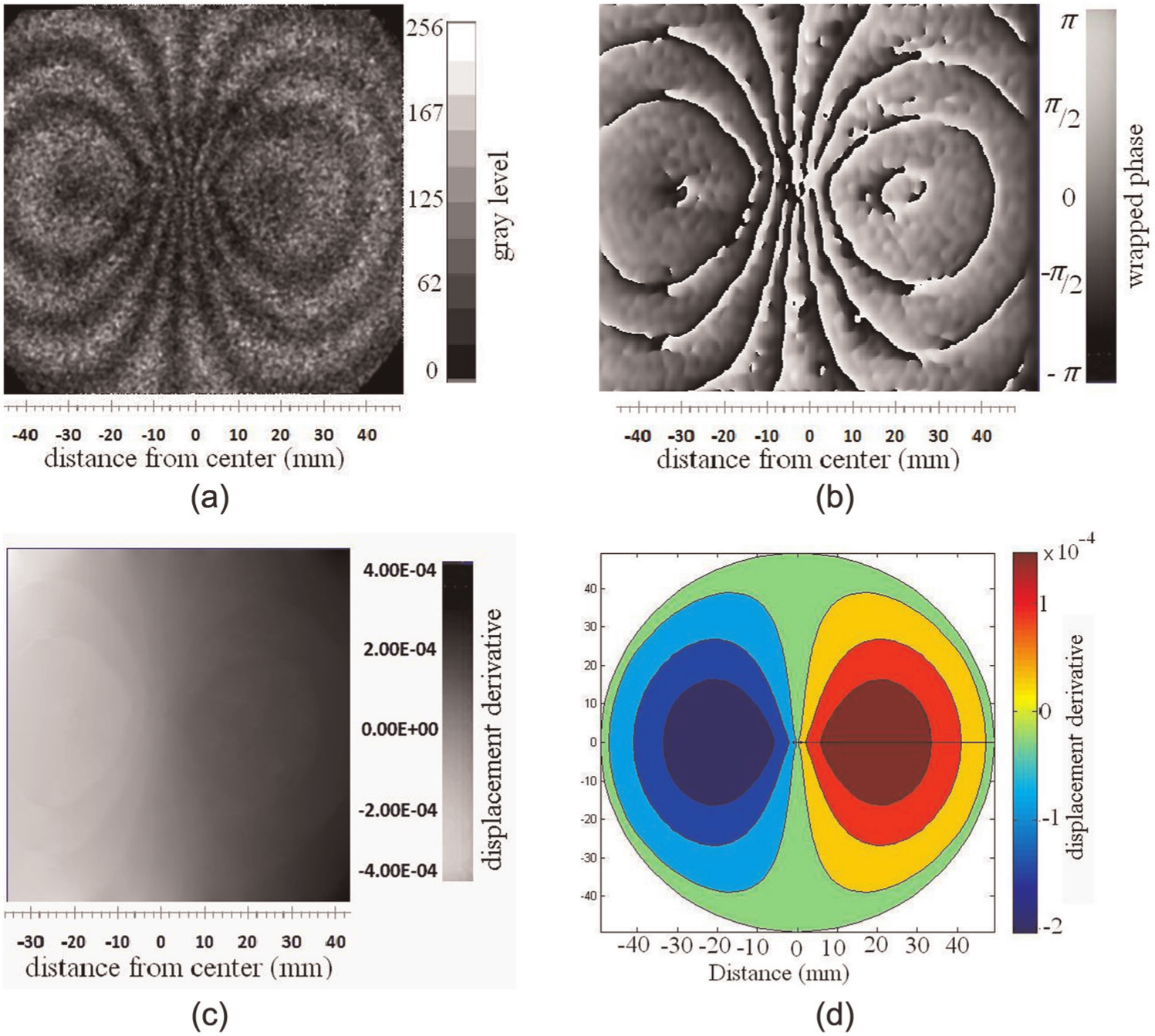
Results of the mechanical loading of the circular plate: (a) shearography fringe patterns, (b) wrapped phase map, (c) unwrapped phase map, and (d) FEM.
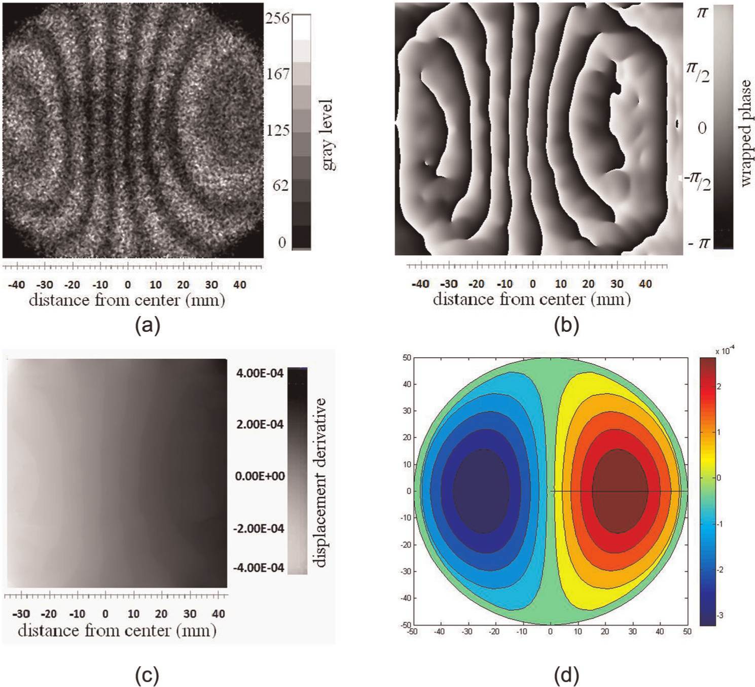
Results of the thermal loading of the circular plate: (a) shearography fringe patterns, (b) wrapped phase map, (c) unwrapped phase map, and (d) FEM.
Because the phase difference between every two neighbor dark fringes is Δ = 2π, according to equation (7), for a pair of consecutive fringes
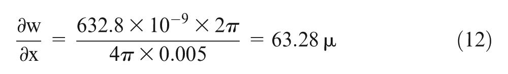
So the difference of
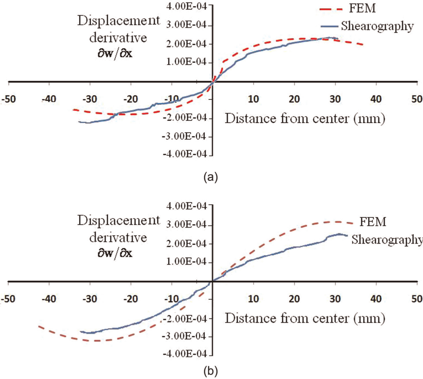
Displacement derivatives through the center of the circular plate in the cases of thermal and mechanical loadings: (a) mechanical loading and (b) thermal loading.
As it can be seen, the mechanical loading creates a relatively good agreement between the experiment and analysis. But in the thermal loading, there are some differences. The main reason is that the parameters of the thermal loading (e.g. heating and cooling rates and environmental conditions) cannot be controlled precisely.
Comparing the experiments with FE results shows that the FE analysis predicts higher values for thermal strains. This means that the heat loss is higher than that we considered. The possible reason may be the other sources of the heat loss, such as conduction between the test plate and the fixture or higher coefficient of convection. Another source may be the amount of heat input to the test plate that may not be linearly increased as it is considered in the FE analysis.
So, to reach an appropriate FEM model with reasonable accuracy, the heating and heat loss parameters should be well adjusted at first.
Denoising the fringe patterns
Shearographic fringe patterns calculated by equation (3) are strangely affected by noise term
Modeling and testing of the defects
Defects, like delaminations, represent the separation between two adjacent layers of the material. In this study, the presence of such defects was simulated by flat-bottom holes, produced with different sizes and depths from the tested surface. The test specimen was made of a 5-mm-thick Plexiglas plate. Two flat-bottom holes with a diameter of 15 and 10 mm were drilled up to a depth of 4.5 and 4 mm, so the delaminated surface is observed in 0.5 and 1 mm from the opposite surface. The 15-mm-diameter hole is shown in Figure 7. Thermal loading was performed using thermal light described in the previous section, and the shearography standard images were taken while cooling down the specimen to room temperature.
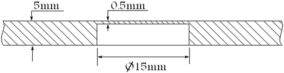
The 15-mm-diameter delamination modeled by flat-bottom hole.
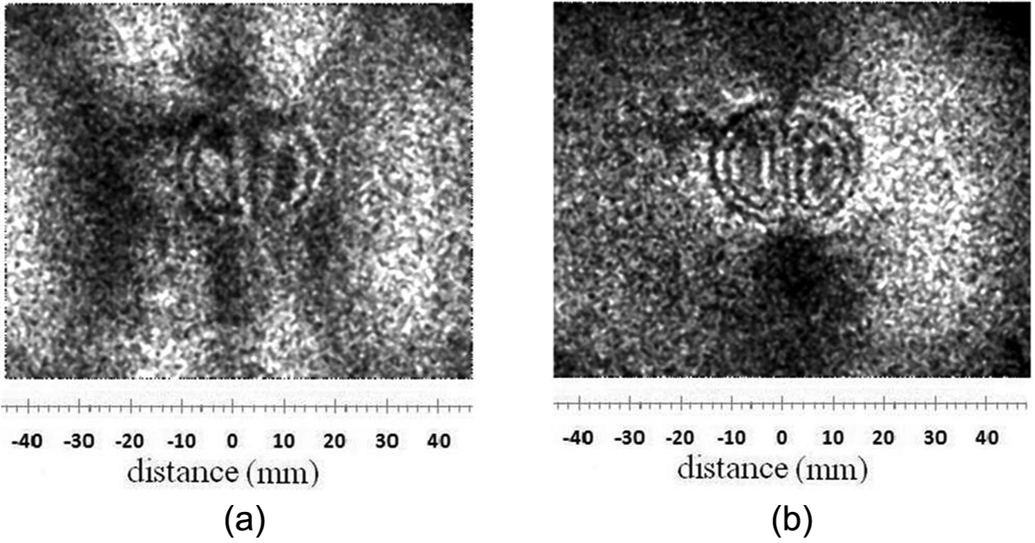
The shearographic correlation fringe pattern and phase map of Figure 7 are shown in Figure 8(a) and (b), respectively. The fringe patterns were taken after 6 s of cooling.
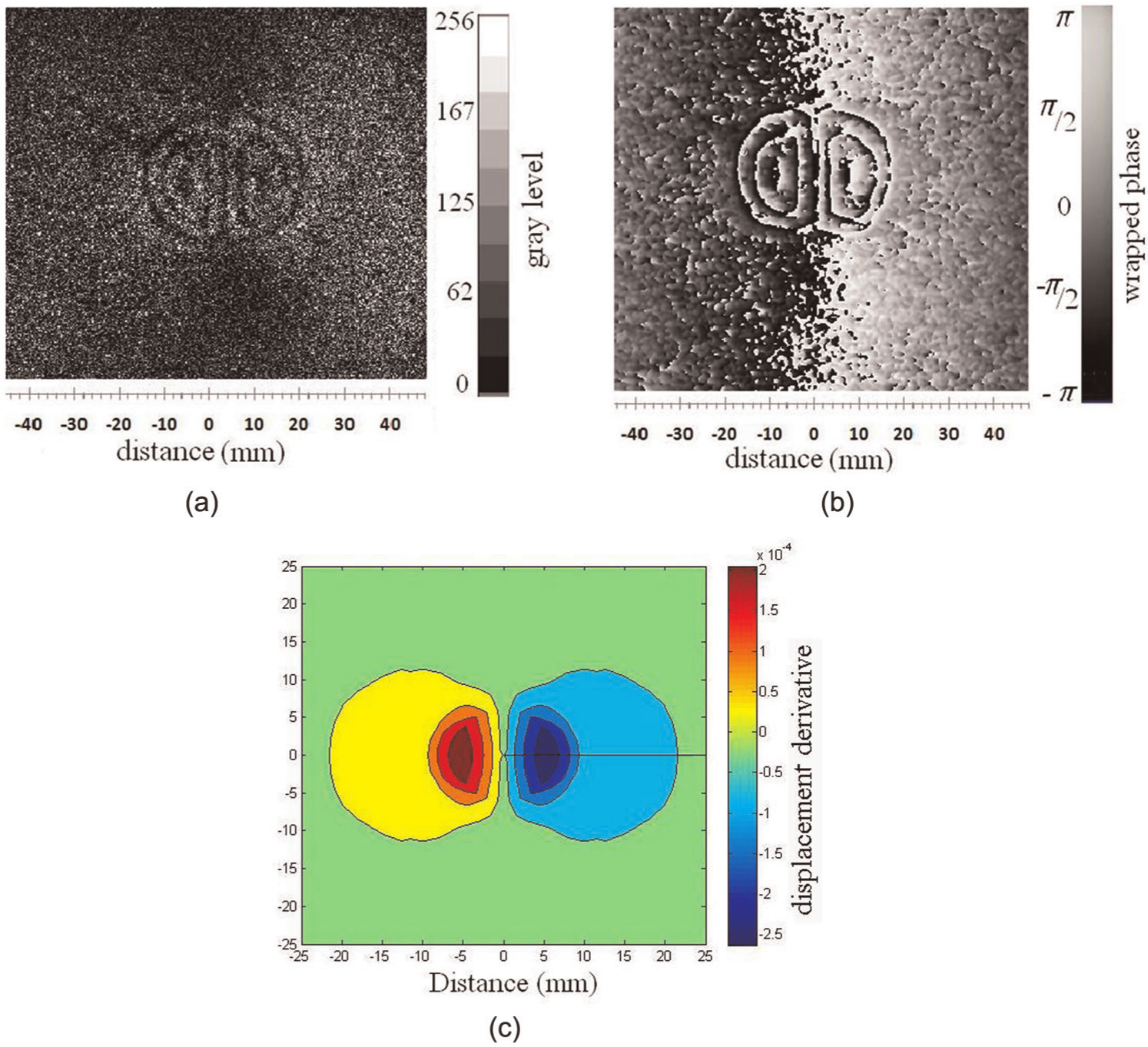
Testing results of 15-mm-diameter flat-bottom hole: (a) shearography fringe pattern, (b) phase map, and (c) FEM.
FE analysis of the 15-mm-diameter flat-bottom hole was performed according to the proposed trend in section “Principles of shearography,” and the relevant FEM contour of displacement derivative
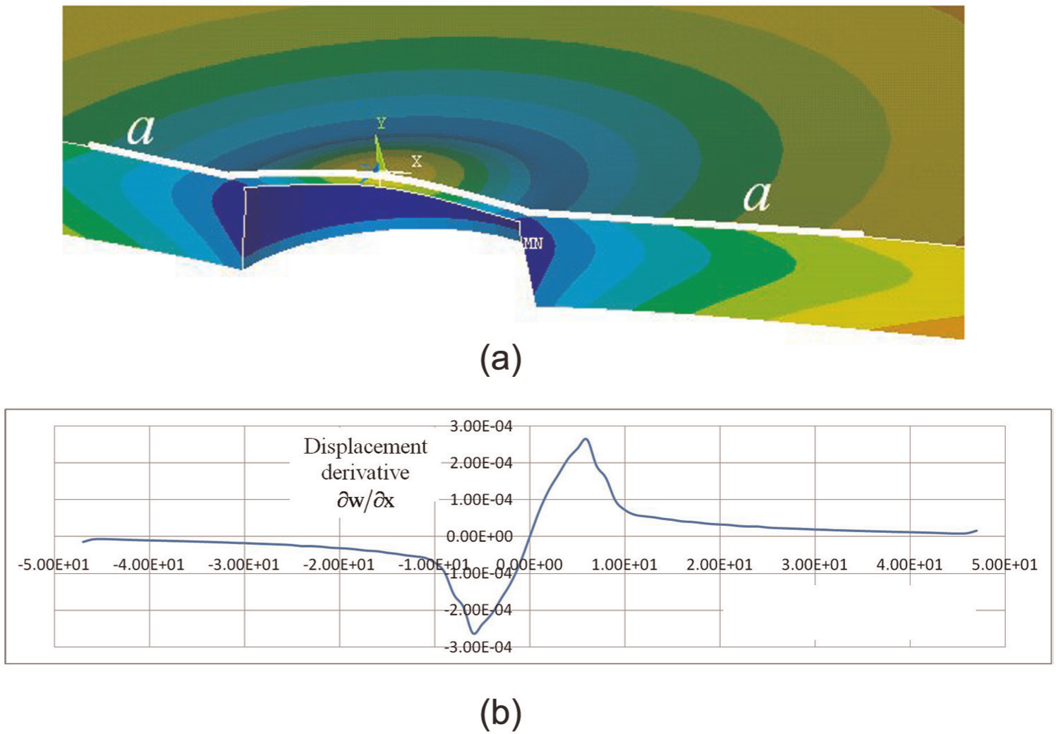
Displacement contour and derivative of the 15-mm-diameter hole: (a) displacement contour and (b) displacement derivative along the axis a–a.
As it is shown, the maximum of
Such a trend is repeated for a 10-mm-diameter flat-bottom hole. As mentioned before, for this case, the depth of the defect is supposed to be 1 mm. The shearography correlation fringe, phase map, and relevant FE results are shown in Figure 10.
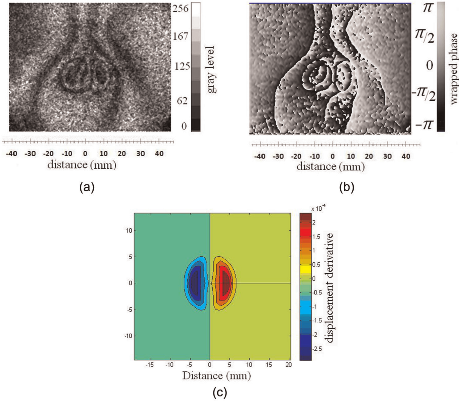
Testing results of 10-mm-diameter flat-bottom hole: (a) shearography fringe pattern, (b) phase map, and (c) FEM.
Figure 10(a) shows that increasing depth of the defect from imaged surface to 1 mm strongly reduces the fringe visibility and also leads to more disagreement between FEM and the experiment. The conclusion is that the accurate FE modeling can be performed for modeling shearograms in the case of shallow defects in polymer material by adjusting the proper loading data.
Effect of the thermal loading parameters
Based on the experiments and the FE modeling with reasonable accuracy proposed before, in this section, a comprehensive study on the effects of the thermal loading parameters to the defect detection is implemented. To achieve this, the visibility of the fringe patterns for different numbers of fringes is initially studied. For the current case study, shearograms were taken while cooling down the specimen continuously. Figure 11 shows different fringe patterns, produced while cooling down the 15-mm-diameter flat-bottom hole. It shows that if the number of fringes becomes more than 7, the fringe patterns would be invisible. Imposing the thermal loading parameters (heating duration and cooling time) of each case of Figure 11 to the FE model indicates a good agreement by considering the proper loading data.
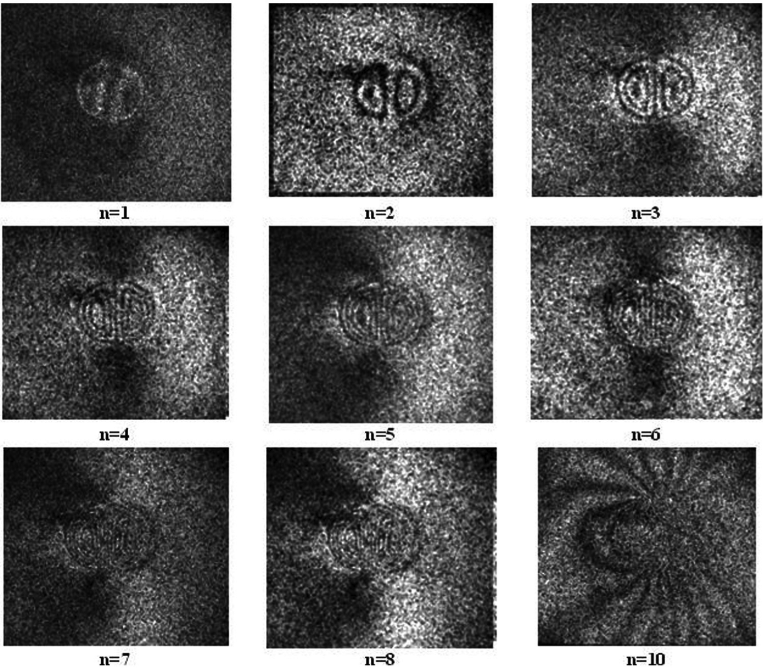
Visibility of different numbers of fringes, captured while cooling down the specimen.
So for this case, the visibility of the fringe pattern can be predicted by FE analysis. The effects of heating time, cooling time, light power, and heating direction on fringe pattern visibility are discussed here.
Heating time
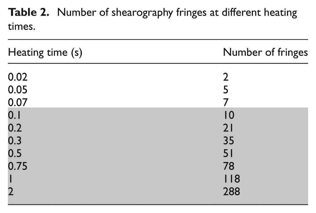
The illumination time was set from 0.02 (flash) to 2 s according to Table 2. For all of the cases, an appropriate FE analysis was run, and the final results are presented. In each case, the number of fringes was derived right after the specimen was heated up. The shaded squares mean that the fringe pattern is predicted to be invisible in the experimental test.
Number of shearography fringes at different heating times.
Cooling time
Shearograms were captured while cooling down the specimen, heated at different heating times according to Table 3. The number of fringes is calculated as a function of cooling time at different heating times by FE analysis.
Number of fringes at different cooling times.
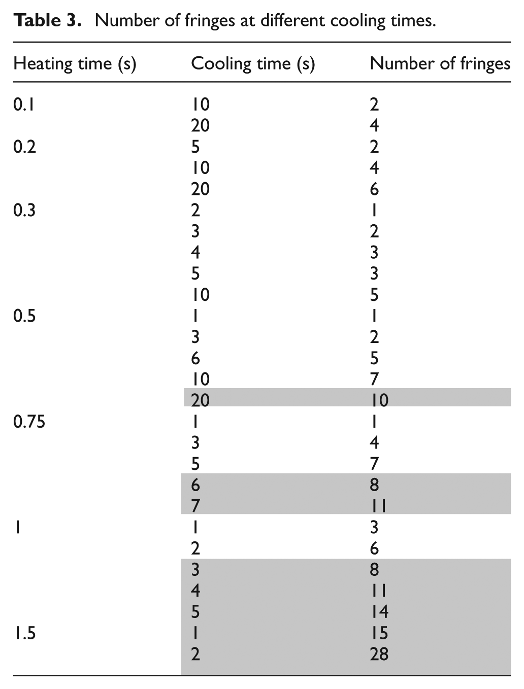
Invisible fringe patterns are illustrated with shaded squares. The combination of heating and cooling times is shown in Figure 12. It shows that for this case, if the cooling time is more than a border line, the fringe pattern is not visible anymore. It also has been shown that if the heating time is more than 1.5 s, the fringe pattern is not visible any longer but can be resolved by capturing the first image with a short delay after heating up. However, over heating makes the entire surrounding area of the defect to be thermally expanded leading to poor visibility of the fringe patterns. Figure 12 can be developed for different defect sizes and depths to find the best heating and cooling times in order to obtain good results from the shearography test.
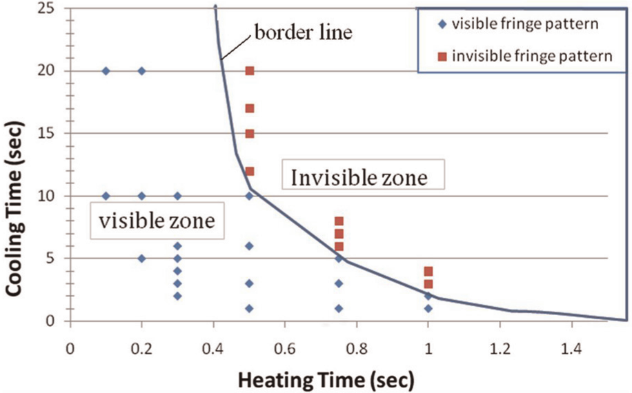
Visibility of fringe pattern for different heating and cooling times.
Heating direction
The test plate was thermally loaded on the front (outside) and both sides. The resultant correlation fringe patterns are shown in Figure 13. As it can be seen, if the plate is thermally loaded from both sides simultaneously, the effects of bending of the surrounding area would be eliminated, and the fringe pattern visibility becomes better.
Correlation fringe patterns for thermal loading on (a) single side and (b) both sides
Effect of shearing distance
The shearing distance is an important factor, which is related to the measuring accuracy and sensitivity. A shearography test of the 15-mm-diameter flat-bottom hole was performed with three shearing amounts of 2.5, 5, and 10 mm. In each case, the thermal loading of the specimen was 1 s of heating and then 1 s of cooling. The resultant shearograms are shown in Figure 14. The results show that the fringe quality is poor in the case of small shearing size (δ = 2.5 mm), and also the number of fringes increases with an increasing shearing distance.
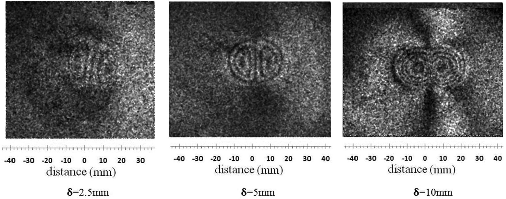
Shearograms for 15-mm-diameter flat-bottom hole with different shearing sizes.
The smaller the shearing amount, the higher the measuring accuracy. But a very small shearing amount creates a poor contrast of the fringe pattern or no fringes at all due to the correlation coefficient. 29 In addition, a larger thermal loading should be applied if the shear value is small. Increasing the loading amount leads to the speckle decorrelation. Mainly due to speckle decorrelation effects, the resulting phase fringe patterns are strongly affected by noise that must somehow be dealt with in order to be able to evaluate the measured phase fringe patterns. If the extent of decorrelation is greater than the speckle size, it eventually leads to a complete loss of fringes. On the other hand, choosing a suitable shearing size is more related to the image width rather than the defect size. So in the shearography tests, in order to reach a good result, it is better to choose a reasonable shearing distance (not less than 1% and not more than 5% of the investigated area), and the specimen should be loaded as low as possible. In this experiment, 5-mm shear and 0.05-s flash warming from both sides result into the best fringe quality.
Conclusion
This article presents a numerical–experimental method to study the effects of thermal loading parameters in the shearography test of polymer materials. In this regard, a numerical method was developed to simulate shearographic fringe patterns using FE analysis. The modeling method was evaluated using experimental tests on a Plexiglas circle subjected to the thermal and mechanical loadings. The proposed method was then applied to the flat-bottom holes, indicating internal defects of the material.
Based on the approved models and experimental data, the comprehensive study of the thermal loading parameters was conducted. According to this study, the following conclusions can be made:
Displacement derivatives predicted by FEM analysis are higher than that of experimental data.
Increasing the depth of the defect to 1 mm from the imaged surface decreases the fringe pattern quality and creates more mismatches between FEM and the experiment. FEM can model shearograms for cases where defects are near the imaged surface.
To reach visible fringe patterns by means of the heating process, the duration of illumination is limited to several percents of a second; the heating time is related to the light power, thermal properties of the test piece, and testing area. In the Plexiglas, it should be less than 0.07 s with a light power of 250 W.
Shearograms of a defected test plate can be properly achieved while cooling down the system, but it is important to keep heating and cooling times below a border line that can be extracted from simulation or experiments.
Heating both sides leads to better results due to eliminating the bending effects in the sounding area of the defects.
To get high contrast fringes with a reasonable accuracy, it is better to keep the shearing amount at a few percent of the image size. In the current study, considering the shearing amount at about 5 mm yields good results.
To prevent undesirable noise generation due to speckle decorrelation, the induced load should be kept as low as possible.
Footnotes
Funding
This research received no specific grant from any funding agency in the public, commercial, or not-for-profit sectors.