Prediction of workpiece dynamic motion using an optimized artificial neural network

Abstract

A machining fixture is an element used to hold the workpiece in the desired position and orientation during machining. The overall machining error in a workpiece is a result of different sources of errors in a workpiece–fixture system. One among them is the motion of the workpiece under the action of cutting forces. Evaluation of this dynamic motion is essential for the determination of the overall machining error. Most commonly, the finite element method is employed to compute the workpiece dynamic motion. During optimization of fixture layout, a large number of layouts are generated and the workpiece dynamic motion must be computed for each of the layouts. In such cases, use of the finite element method is prohibitive because of the long computation time required. Also, the results of the finite element analysis are susceptible to different parameters used in the analysis. Hence, an alternate and efficient methodology is necessary to determine the workpiece displacement for a given fixture layout. This article proposes a method of using an artificial neural network for the prediction of workpiece dynamic motion. Different layouts are obtained using a modular fixture and actual machining is performed on the workpiece. For each layout, the workpiece dynamic motion is computed at select datum points and an artificial neural network is trained with these data. To achieve better prediction capability of the artificial neural network and minimize different forms of errors in training and generalization, critical parameters of the artificial neural network are optimized using a genetic algorithm. Then, this optimized network is employed to predict the workpiece dynamic motion for any arbitrary layout. Results show that the optimized artificial neural network is capable of predicting the workpiece dynamic motion with acceptable accuracy (maximum absolute relative error 9.71%). This method, hence, can serve as an economical means of computing the overall machining error during optimization of fixture layouts.

Introduction

With more emphasis on the quality of parts, fixture design has evolved as an important area of research. As a workholding device, a machining fixture is responsible for ensuring that the workpiece is held in the required position and orientation during machining. Any error in the fixture design is directly translated as the machining error of the workpiece and hence the machining accuracy is lost. In a workpiece–fixture system (WFS), many sources of error contribute to the final machining error of the workpiece. These include, but are not limited to, the geometric error at locators, compliance at the workpiece–locator contact bulk elasticity of workpiece and workpiece dynamic motion (WDM). As cutting forces are time varying, the workpiece being machined experiences dynamic motion and this has a significant contribution to the final machining error. Because of this reason, many researchers have investigated the effect of the workpiece dynamics and the ways to minimize the same in order to improve workpiece accuracy.

Studies on the dynamics aspect of WFS focus on the modeling of the workpiece fixture contacts, analyzing the dynamic behavior of WFS and optimizing the fixture parameters for minimizing the dynamic motion. Daimon et al. ¹ presented a method for selecting supports to improve workpiece dynamic rigidity based on a finite element analysis. Mittal et al. ² used the dynamic analysis and design system (DADS) software for analyzing the workpiece dynamics. In their work, the workpiece–fixture contact was modeled using a lumped spring actuator element. Liao and Hu ³ extended this work by considering the structural compliance of the workpiece and contact friction. For this purpose, the finite element method (FEM) was used in conjunction with the DADS software. Liao and Hu ⁴ employed a translational spring damper actuator model to represent the workpiece–fixture contact in an attempt to determine the clamping force, clamping point and clamping sequence in the case of time varying machining loads. The FEM was employed to determine the modal coordinates considering the elasticity of the workpiece and locator. Fang et al. ⁵ presented a model to study friction damping considering the dynamics of both workpiece and fixture elements. They attributed the phenomenon of interface locking for the dependency of friction damping on clamping forces.

Deiab and Elbestawi ⁶ analyzed the effect of chip removal on the WFS dynamics using a finite element model. Liu and Strong ⁷ presented a linear programming (LP)-based fixture verification method considering the dynamics of the fixture workpiece system. However, they considered both workpiece and fixture elements to be rigid. Motlagh et al. ⁸ employed a modified version of the Armstrong friction model to study the WFS behavior under dynamic conditions.

The common limitation of the above works is that they did not address the methods of achieving the minimum dynamic motion of the workpiece under the given conditions.

Since the WDM can be minimized by optimizing either or both the fixture layout and clamping forces, attempts have been made on this front. Using a rigid body dynamic model, Li and Melkote ⁹ optimized the fixture layout for minimum WDM. This work did not consider the elasticity of the workpiece and fixture elements. Deng and Melkote ¹⁰ determined the minimum clamping forces required for fixturing stability using particle swarm optimization (PSO). In this work, the contact elasticity model was used to check the stability of the workpiece under dynamic conditions. Padmanaban and Prabhaharan ¹¹ used a genetic algorithm (GA) and ant colony algorithm (ACA), separately, to determine the optimal positions of fixture elements to achieve minimum dynamic displacement of the workpiece. However, in this work, the search space was limited to the node numbers of a finite element model. To overcome this drawback, Padmanaban et al. ¹² employed a continuous optimization scheme based on the ACA to optimize the fixture layout under dynamic conditions. In this work, the search space was defined as the physical coordinates, thereby enabling a more effective search. In both of these works, simple two-dimensional geometries were considered.

Though these works have provided a solid foundation on the analysis of WFS dynamics, some shortfalls can be noted. First, a systematic methodology to relate the WDM to the machining tolerance is not provided. This is required because, with the machining tolerance given, if the WDM is known a priori, following the principles of tolerance accumulation, one can determine how much error can be ‘shared’ by the other error sources mentioned earlier.

Second, limitation lies in the approach to layout optimization. Some of the above works sought to optimize the layout or clamping forces in an attempt to minimize the WDM. But most of these studies employed finite element models and are not based on experimental methods. Using the FEM has some limitations. To achieve a realistic model of workpiece–fixture contact, both of them must be modeled as elastic members. For such modeling, even a static analysis based on the FEM is computationally intensive. ¹³ For dynamic analyses, this problem is more acute. It is not uncommon to see the software requiring hours of time for completing a single iteration. In an optimization process, the number of layouts is so large in number that analyzing each layout using the FEM is prohibitive. The other limitation is in the form of non-uniqueness of the results of the FEM-based analyses. It is known that the results of a finite element analysis depend largely on the parameters used in the study. This may include modeling of contacts, mesh size and element shape and type. ¹⁴ In other words, different finite element analyses performed on the same WFS can produce different results, the degree of variation being case-based.

Owing to the above reasons, a computationally efficient method of determining the WDM is warranted. Such a method should be capable of simulating the actual machining conditions in a better way and it should also be economical in terms of computational time.

This article proposes the use of an optimized artificial neural network (ANN) for predicting the dynamic motion of a real, three dimensional workpiece. The dynamics of a workpiece–fixture system is complex and there is no direct mathematical relationship available to correlate the fixture layout to the workpiece motion owing to dynamics. It is because of this reason that the use of ANNs is promising for this application of predicting WDM. In the present work, the case of a prismatic workpiece being machined in a typical 3-2-1 fixture set-up is considered and the WDM for different layouts is captured experimentally. The prediction accuracy of an ANN is influenced by various parameters used in its architecture. Hence, a suitable model of ANN is identified and its critical parameters are optimized using a GA. Then the network is trained with the experimental data so that it can predict the WDM for an arbitrarily generated layout.

Dynamic motion and machining error

The workpiece is subject to time-varying cutting forces during machining. This induces vibration in the workpiece and the vibration amplitude depends on many factors, like fixture design, machine tool rigidity and cutting conditions. Figure 1 depicts a representative workpiece surface that vibrates. The cutter path is pre-defined and does not change during cutting. But, since the workpiece has displaced owing to vibration, the cutter “meets” the workpiece at a point different than the intended one. This point is away by a distance shown exaggerated as δ and this deviation directly amounts to an error. It should be noted that the workpiece vibratory motion is possible in all six degrees of freedom (three translations and three rotations) and, hence, the error, called a dynamics related error, is a vector, written as δ m _d given by

Figure 1.

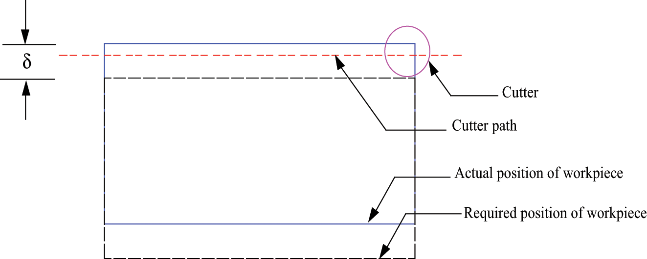
Error due to dynamic motion of the workpiece.

$$\delta {\mathit{m}}_{\text{d}}={\left\{{\delta }_{\text{x}}{\delta }_{\text{y}}{\delta }_{\text{z}}{\theta }_{\text{x}}{\theta }_{\text{y}}{\theta }_{\text{z}}\right\}}^T$$

(1)

But, depending on how the tolerance is specified in the critical machining feature of the workpiece, dynamic motion along one or more directions would be of interest. For example, if the tolerance is specified on the Y direction, only δ_y requires to be considered.

As mentioned above, since the motion of the cutting tool is fixed for a given machining operation, evaluation of machining error can be equivalently transformed into the evaluation of the variation of the processing datum with respect to the global coordinate system (GCS). ¹⁵ Variation of the processing datum is measured by computing the variation of certain representative points along the datum. These points are known as processing datum points. Maximum variation experienced among those points is the final machining error of the critical feature of the workpiece. Stated mathematically

$$\delta m_{\text{i}}=\max (\mathrm{abs}(\delta m_{1,}\delta m_{2,}\dots \delta m_{\text{n}}))$$

(2)

where i refers to the X, Y, Z directions and n is the number of processing datum points.

Proposed approach

The task at hand is to arrive at a new, computationally efficient methodology for determining the WDM for a given fixture layout. To achieve the stated aim, this article proposes an ANN-based method depicted in Figure 2. The method involves the following steps.

Figure 2.

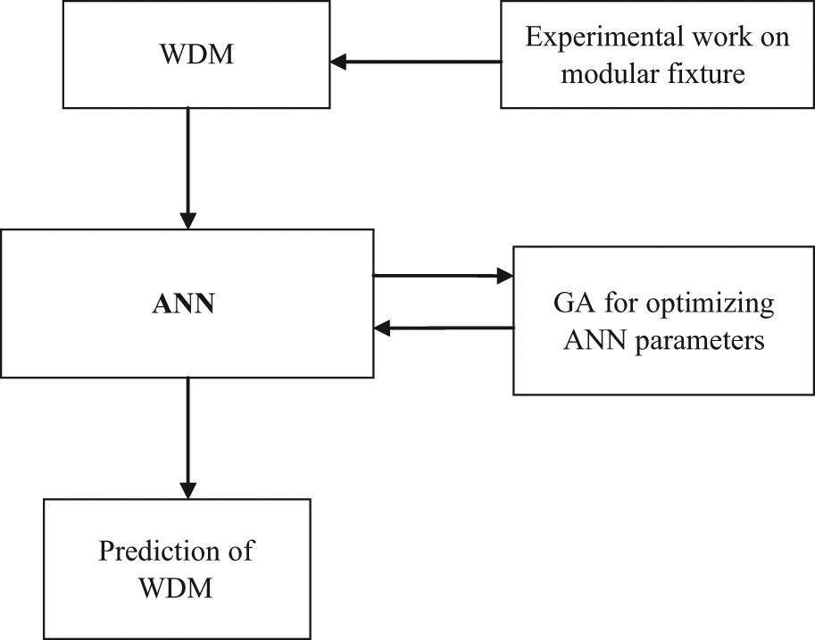
Methodology for the prediction of WDM using an ANN.

1. Set up a modular fixture so that different layouts can be achieved.

2. Perform machining on the workpiece with different layouts.

3. Measure the dynamic motion of the workpiece at the datum points.

4. Identify a suitable ANN and optimize its critical parameters.

5. Train the network with the data of WDM obtained experimentally.

6. Use the ANN for prediction of workpiece motion for a required layout.

Numerical illustration

Problem definition

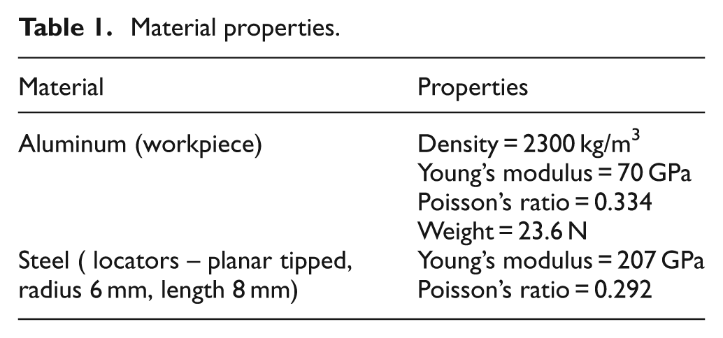
The study involves a WFS as shown in Figure 3. A through slot of size 80 mm × 60 mm is to be milled on a cubical aluminum block of side 101.6 mm. Typical a 3-2-1 locating scheme is followed and hence the fixture consists of six locators denoted as L₁…L₆. Locators L₁, L₂ and L₃ are in the primary datum, L₄ and L₅ are in the secondary datum and L₆ is in the tertiary datum. Two clamps C₁ and C₂ exert the required clamping forces. The material properties of workpiece and fixture elements are given in Table 1.

Figure 3.

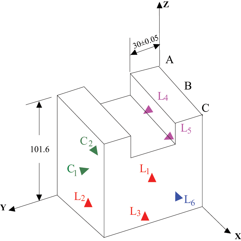
WFS under study.

Table 1.

Material properties.

Material	Properties
Aluminum (workpiece)	Density = 2300 kg/m3
	Young’s modulus = 70 GPa
	Poisson’s ratio = 0.334
	Weight = 23.6 N
Steel ( locators – planar tipped, radius 6 mm, length 8 mm)	Young’s modulus = 207 GPaPoisson’s ratio = 0.292

The critical feature in this workpiece is the distance of the slot from the right end, marked as 30 ± 0.05 mm. Since the machining tolerance is specified along the Y direction, the WDM along Y direction alone is of interest. Therefore, in the subsequent sections of the article, WDM represents WDM in the Y direction. The problem at hand is to predict the dynamic motion of the workpiece for a given layout with the least possible error.

Experimental set-up

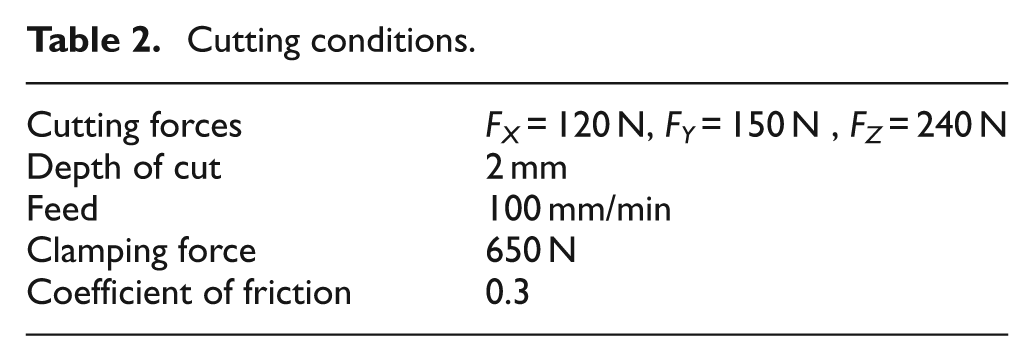
Since the WDM is to be captured for different layouts, a modular fixture is employed. This fixture, shown in Figure 4, has provision for locators and clamps to be placed according to the requirement. The workpiece is held in this fixture and clamped by means of screw clamps. This fixture is held in an ARIX vertical machining center and end milling of the slot is carried out on the workpiece. This machining center has a capacity of 1000 mm × 500 mm × 500 mm along the longitudinal, cross and vertical axes, respectively, and a maximum feed rate of 4000 mm/min with a table size of 1270 mm × 330 mm. Table 2 shows the cutting conditions used in the study. The time-varying machining forces in X, Y and Z directions during milling are shown in Figure 5. It can be seen that maximum forces are encountered during the initial instant of machining. After this point in time, machining forces are lesser in magnitude. The machining forces given in Table 2 are the maximum forces encountered during milling.

Figure 4.

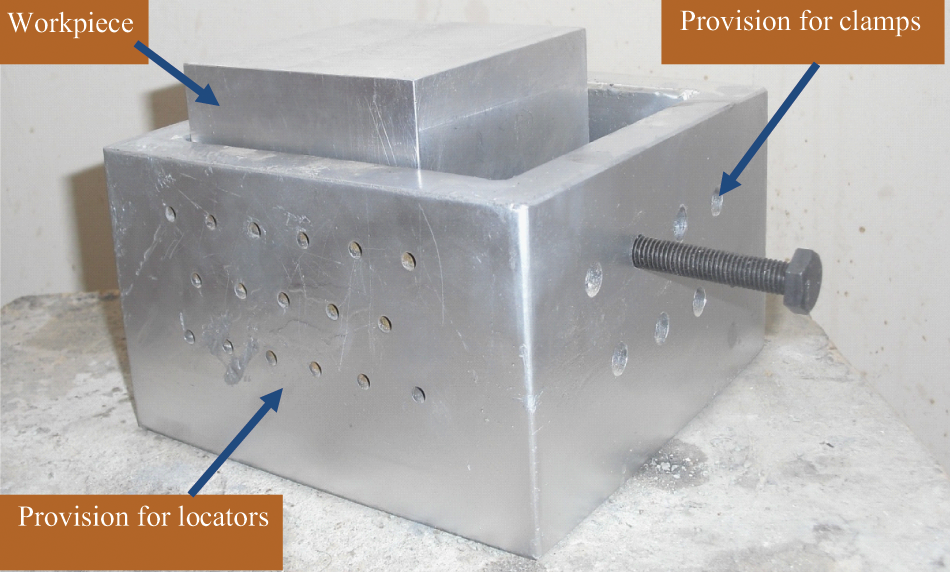
Modular fixture set-up.

Table 2.

Cutting conditions.

Cutting forces	F X  = 120 N, F Y  = 150 N, F Z  = 240 N
Depth of cut	2 mm
Feed	100 mm/min
Clamping force	650 N
Coefficient of friction	0.3

Figure 5.

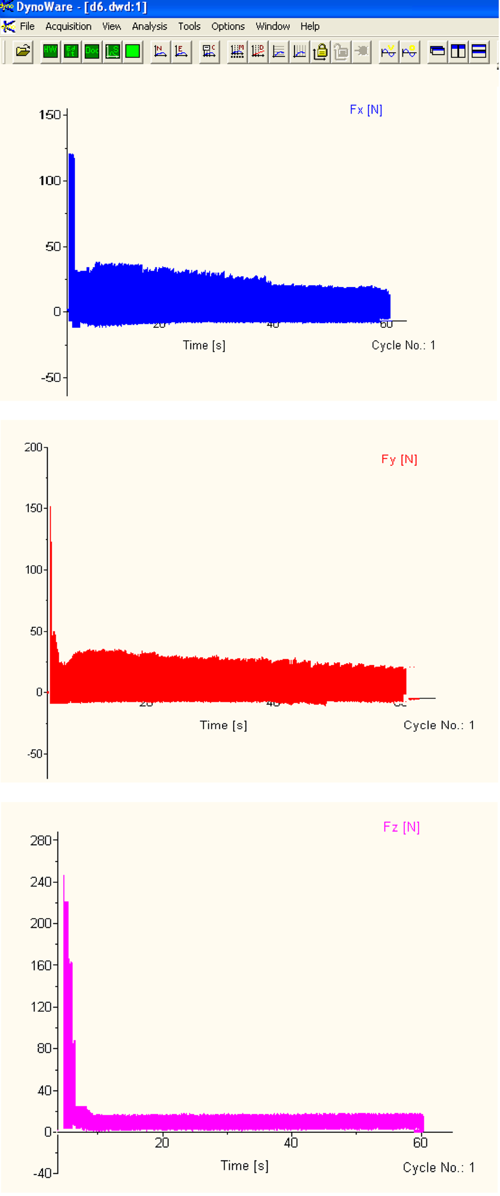
Cutting forces during machining.

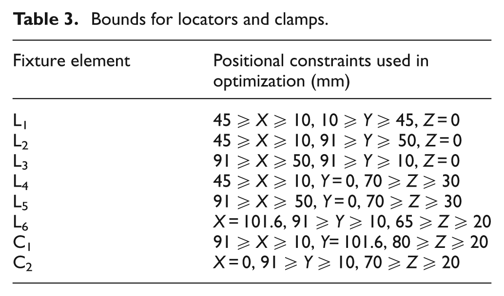
Before the actual start of machining, the position of each of the six locators and two clamps have to be decided. This has to be done without violating logic and established principles of locating. It is well known from the principles of locating that the machining forces should always be directed against a locator rather than a clamp. Also, two locators cannot be coincident. The third requirement is that the locators/clamp cannot be placed at the corner or edge of the workpiece to avoid instability. These requirements have been taken into consideration while fixing the bounds for the present case and these bounds are shown in Table 3.

Table 3.

Bounds for locators and clamps.

Fixture element	Positional constraints used in optimization (mm)
L1	45 ≥ X ≥ 10, 10 ≥ Y ≥ 45, Z = 0
L2	45 ≥ X ≥ 10, 91 ≥ Y ≥ 50, Z = 0
L3	91 ≥ X ≥ 50, 91 ≥ Y ≥ 10, Z = 0
L4	45 ≥ X ≥ 10, Y = 0, 70 ≥ Z ≥ 30
L5	91 ≥ X ≥ 50, Y = 0, 70 ≥ Z ≥ 30
L6	X = 101.6, 91 ≥ Y ≥ 10, 65 ≥ Z ≥ 20
C1	91 ≥ X ≥ 10, Y= 101.6, 80 ≥ Z ≥ 20
C2	X = 0, 91 ≥ Y ≥ 10, 70 ≥ Z ≥ 20

The number of experiments to be conducted (number of different layouts to be used in the experiment for forming the data pool) was obtained based on the concepts of design of experiments (DoE). The problem with factorial design is that the combinations increase exponentially as the factors increase. In the present case, there are 16 factors (see ‘Modeling of the ANN’) and, hence, use of full factorial design would lead to a prohibitively large number of experiments and therefore cannot be adopted. Hence, the fractional factorial design (FFD) model is adopted in this work. Using the Design Expert software (version 7.0.0), for two levels with 16 factors, it was found that 128 experiments must be conducted. ¹⁶ For each of these layouts, the WDM must be computed. In all the experiments, it must be ensured that the coordinates of each locator and clamp satisfy the bounds given in Table 3.

During the experiment, the locators and clamps are fixed as per the layout generated. The workpiece is held in this layout within the machining fixture and machining is done using an end mill. For one complete stroke of the end mill, the workpiece displacement is computed at each of the processing datum points A, B and C. Since three datum points are considered, three accelerometers in conjunction with a multichannel data acquisition system (National Instruments) are used to acquire the workpiece acceleration. These acceleration signals are processed and converted to displacement data using the LabVIEW^® software. The data acquisition set-up is shown schematically in Figure 6 and pictorially in Figure 7.

Figure 6.

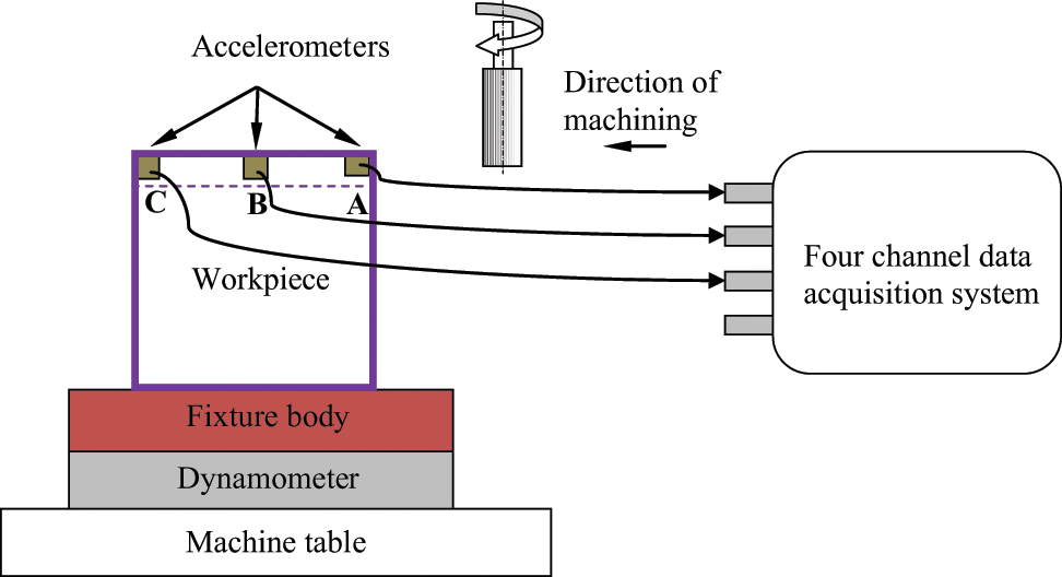
Schematic of measuring the WDM.

Figure 7.

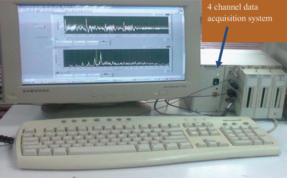
Data acquisition set-up.

Since the experiment needs to be carried out for 128 different layouts, it would be uneconomical if the complete slot of 40 mm width were to be machined for taking one reading. Hence, considering economic aspects, one complete stroke of the end mill is executed and this is assumed to represent the machining of an entire width of the slot.

Experimental results

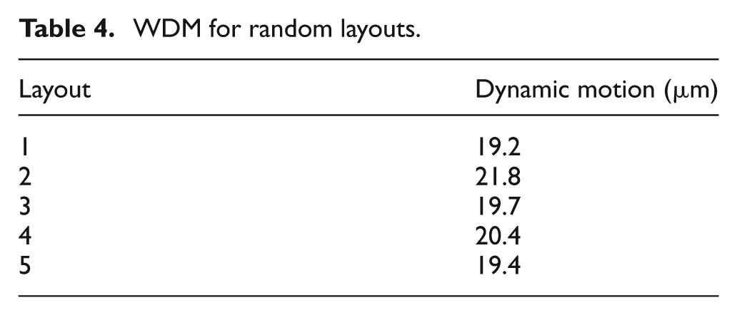
The WDM during machining is depicted in Figure 8. Figure 8(a) shows the WDM at a given instant and Figure 8(b) shows the variation of WDM at the three datum points for one complete stroke of the end mill. As can be seen, the magnitude of this motion is different at the datum points. For example, point A experiences a maximum value of 0.017 mm at the start of the cutting. As machining progresses and the cutter moves away from A, the magnitude gradually decreases. The pattern of change at the datum points seems to suggest that, as the cutter comes closer to a datum point, WDM at that datum point reaches its maximum and keeps decreasing after that. It should however, be noted that the trend and magnitudes may be different for a different layout. For example, consider Table 4 which shows the WDM for five randomly generated layouts. It can be seen that these values are significantly higher than the case depicted in Figure 8(b).

Figure 8.

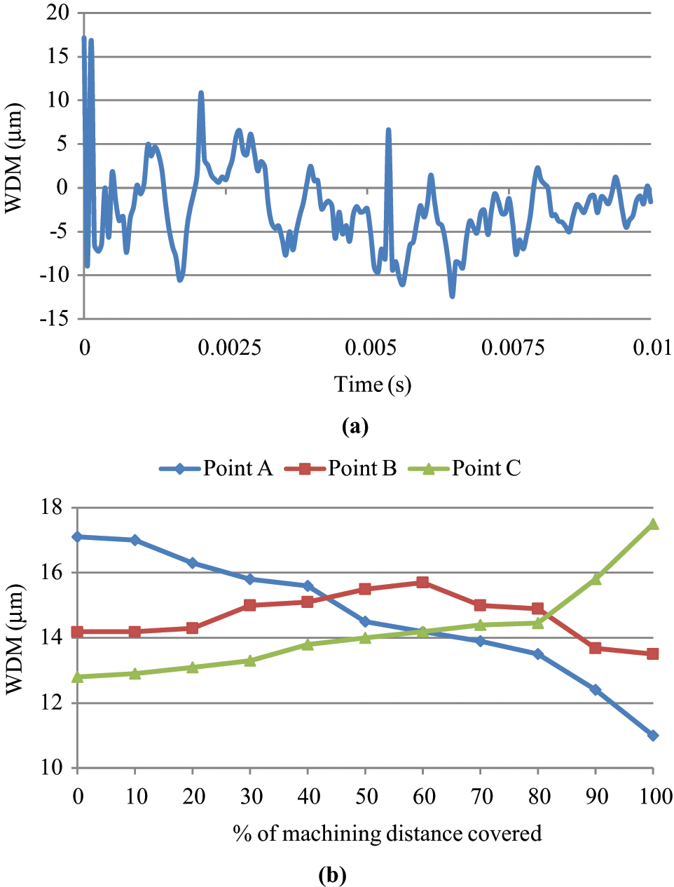
WDM at datum points during machining: (a) instantaneous; (b) along machining length.

Table 4.

WDM for random layouts.

Layout	Dynamic motion (µm)
1	19.2
2	21.8
3	19.7
4	20.4
5	19.4

Prediction of WDM using an ANN

Modeling of the ANN

In this research work, a feed forward ANN with back propagation algorithm ¹⁷ is used for the prediction of WDM. One of the built-in functions of MATLAB, namely the newff, is used for creating the network and the function traingdm is used for training the same. The ANN proposed in this work has a single hidden layer. Transfer functions tansig and purelin are used for the hidden layer and the output layer, respectively. These functions are briefly reviewed in the Appendix.

In the present problem, the objective is to develop an ANN that is capable of predicting the WDM at three datum points for a given fixture layout. Referring to Figure 3, the WFS consists of six locators and two clamps. Hence, the input to the ANN are the X, Y and Z coordinates of these eight elements, and the ANN output will be the WDM at datum points A, B and C. This means that the input vector should be of length 24, and output a vector of length 3. But some of the coordinates get fixed by virtue of their location. Referring to Figure 3 and Table 3, it can be seen that the Z coordinate of L₁, L₂, L₃, Y coordinate of L₄ and L₅, and X coordinate of C₂ are all zero. Similarly, the X coordinate of L₆ and Y coordinate of C₁ are the same (101.6 mm). Since these eight components get fixed, the number of variable input coordinates is reduced from 24 to 16. Figure 9 shows the ANN architecture that accepts 16 inputs and gives the WDM as output.

Figure 9.

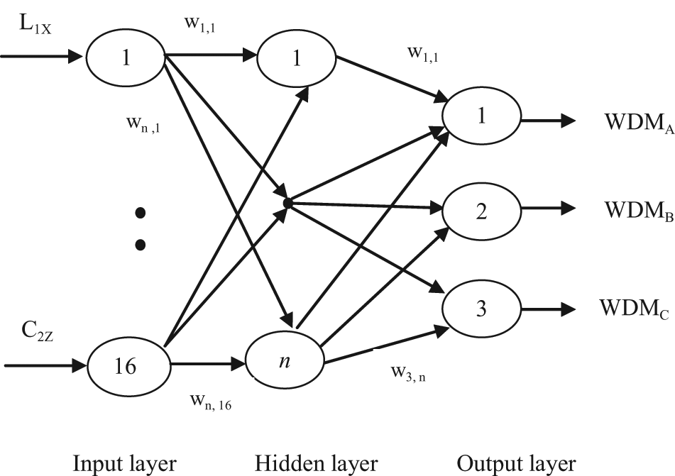
Architecture of the ANN.

Working of the ANN

In an ANN, each input parameter is indicated by a node in the input layer. Each of these inputs in the input vector p is multiplied by its corresponding weight and distributed to each neuron in the hidden layer. These are summed up to give a vector (n^h). This vector is subject to a transfer function (F^h), thereby giving an output at the hidden layer (a^h). Each of these outputs is distributed to each neuron in the output layer, weighted again and summed up to give a vector (n^o). This vector is subject to transfer function (F ^o ), so as to result an output at the output layer (output of the entire network), denoted as a^o. It can be noted that n is used to denote the vector at a given layer before applying the transfer function and a is used to denote the output of the layer after transfer function F is applied to n.

The different weights between two layers can be written in the form of a weight matrix W. If R is the number of input elements and S is the number of neurons in the next (hidden) layer, then W is of size S × R. In general, the weight matrix between the kth and (k–1)th layers, denoted as W^k, is given by

$${\mathbf{W}}^{\mathbf{k}}=\left[\begin{array}{cccc}{w}_{1,1}& w_{1,2}& \mathrm{\dots }& w_{1,R}\\ w_{2,1}& w_{2,2}& \mathrm{\dots }& w_{2,R}\\ \mathrm{\dots }& \mathrm{\dots }& \mathrm{\dots }& \mathrm{\dots }\\ w_{S,1}& w_{S,2}& \mathrm{\dots }& w_{S,R}\end{array}\right]$$

(3)

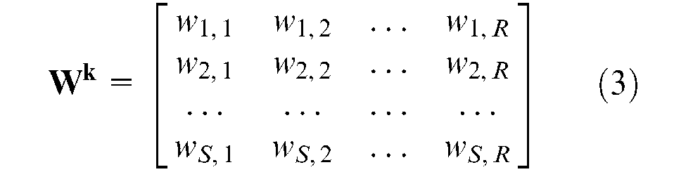
in which w _j,i is the weight whose destination is neuron j in the kth layer and the source of the same being neuron i in the (k–1)th layer. Thus, w_2,1 represents the weight for neuron 2 in the kth layer that comes from neuron 1 in the previous layer (see Figure 9).

With the parameters defined above, the input–output relation for a layer can be written as

$$\mathbf{a}=F(\mathbf{Wp}+\mathbf{b})$$

(4)

where b is the bias vector for the layer.

Equation (4), as applied to the input and hidden layer, will be

$${\mathbf{a}}^{\text{h}}=F^{\text{h}}({\mathbf{W}}^{\text{h}}\mathbf{p}+{\mathbf{b}}^{\text{h}})$$

(5)

and between hidden and output layers will be

$${\mathbf{a}}^{\text{o}}=F^{\text{o}}({\mathbf{W}}^{\text{o}}{\mathbf{a}}^{\text{h}}+{\mathbf{b}}^{\text{o}})$$

(6)

As mentioned in ‘Modeling of the ANN’, the input layer has 16 neurons and the output layer has three neurons. At this stage, the number of neurons in the hidden layer (n _h ) is not known. This will be determined by optimization as explained in ‘Need for optimization of ANN parameters’. With these details, and remembering that the transfer functions tansig and purelin are used for hidden layer and output layer respectively, the ANN employed in the present work can be schematically represented as shown in Figure 10.

Figure 10.

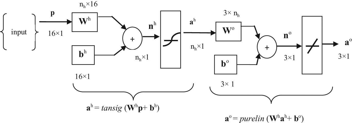
Working scheme of the ANN.

Need for optimization of ANN parameters

Performance of an ANN is affected by different factors and hence, it is imperative to identify and optimize these factors.

Mathworks ¹⁸ reports that for the traingdm function, the performance of the network is very sensitive to the setting of learning rate (LR) and momentum constant (MC) (please refer to Appendix for details). Hence, optimal values of these two parameters need to be determined.

The second factor that warrants attention is the network size. Network size determines the network efficiency and the time taken for learning and generalization. As explained in ‘Modeling of the ANN’, the number of neurons in the input and output layers depend on the number of inputs and output variables, respectively. With the number of neurons in the input and output layers fixed, the network size depends on the number of neurons in the hidden layer (n _h ). The network complexity increases exponentially with respect to the number of neurons in the hidden layer. ¹⁹

The third factor relates to the errors encountered in using an ANN. In the ANN parlance, two types of error are identified. These are the training error and the generalization error. The former refers to the difference between what the ANN must learn and what it has actually learnt. The latter denotes the difference between the ANN predicted value and the actual or target value. For the ANN to be efficient in prediction, it is essential that both these errors are minimized.

Hence, a computationally efficient ANN should possess the following characteristics.

1. Optimal values of learning rate and momentum constant.

2. Optimal number of neurons in the hidden layer.

3. Minimum error in training and generalization.

This requires that the ANN should first be optimized to attain these characteristics. Before optimization is invoked, a suitable objective function must be identified that can collectively represent the above three parameters.

The objective function used by Benardos and Vosniakos ¹⁹ is employed in this work, and the same is given by

$$\Phi =e^{0.001n}(E_{\mathrm{train}}+E_{\mathrm{gen}})$$

(7)

where E _train and E _gen refer to the errors in training and generalization, respectively, and n _h refers to the number of neurons in the hidden layer. Various parameters are available to measure these errors. These include the mean square error (MSE), mean squared error with regularization (MSER) and mean absolute relative error (MARE). This work uses the MARE to measure these errors since it is easier to interpret and does not require scaling or normalization.

On this basis, E _train and E _gen are given by

$$E_{\mathrm{train}}=\frac{\sum _{i=1}^N|(S_{\mathrm{oi}}-S_i)/S_{\mathrm{oi}}|}{N}$$

(8)

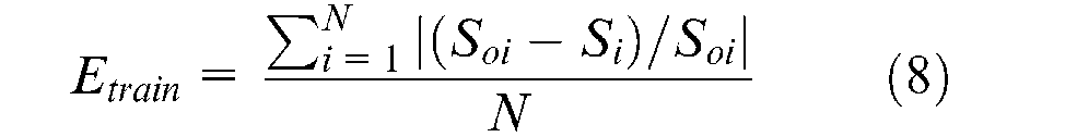
where

S _oi  = target value of the ith training data vector (what the ANN must learn);

S _i  = ANN’s response to the training data vector (what the ANN has actually learnt);

N = the number of training datasets.

Similarly

$$E_{\mathrm{gen}}=\frac{\sum _{i=1}^n|(T_{\mathrm{oi}}-T_i)/T_{\mathrm{oi}}|}{N_t}$$

(9)

where

T _oi  = target value of the ith testing data vector (what the ANN must predict);

T _i  = ANN’s output (what the ANN has actually predicted);

N _t  = number of testing datasets.

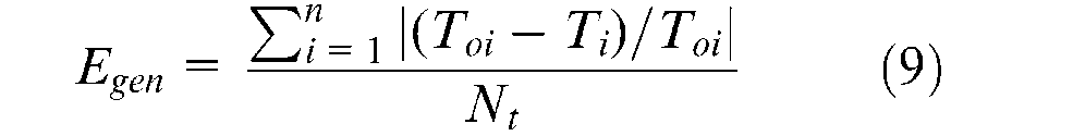
In equation (9), the term inside the modulus symbol is simply the absolute error relative to the target value. This is termed as absolute relative error (ARE).

GA-based optimization of ANN parameters

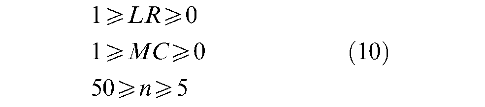
In this work, a GA coded in the MATLAB environment attempts to minimize the function Φ defined by equation (3). It can be noted that minimizing this function serves the twin purposes of a compact network and a minimum error in training and generalization. This problem of optimization can be stated as follows.

Minimize

$$\Phi =e^{0.001n}(E_{\mathrm{train}}+E_{\mathrm{gen}})$$

subject to

$$\begin{array}{c}1\ge \mathrm{LR}\ge 0\\ 1\ge \mathrm{MC}\ge 0\\ 50\ge n\ge 5\end{array}$$

(10)

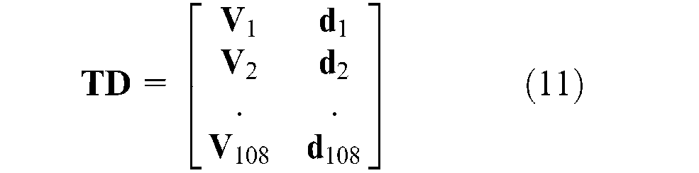
Further to ‘Experimental set-up’, the WDM data is available from 128 experiments. These 128 data must be apportioned for training and generalization. Based on Mathwords ¹⁸ and Benardos and Vosniakos, ¹⁹ 15% of the available data (20 sets of data) are used for generalization and the remaining 108 are used for training.

The training data input to the ANN consists of the details of the ith layout given by V _i and the WDM obtained at the three datum points for each layout, given by d _i . In essence, V _i represents the coordinates of each locator and clamp.

The input to the ANN is hence a matrix TDℜ ^{108 × 19} with the following form

$$\mathbf{T}\mathbf{D}=\left[\begin{array}{cc}{\mathbf{V}}_1& {\mathbf{d}}_1\\ {\mathbf{V}}_2& {\mathbf{d}}_2\\ .& .\\ {\mathbf{V}}_{108}& {\mathbf{d}}_{108}\end{array}\right]$$

(11)

where

$\left[\begin{array}{c}{\mathbf{V}}_i{d}_i\end{array}\right]{\in }^{1\times 19}$ is the input vector for the ith layout, with the coordinate vector

$${\mathbf{V}}_i=\left\{\begin{array}{c}{X}_1{Y}_1...Y_{C2}{Z}_{C2}\end{array}\right\}{\in }^{1\times 16}$$

(12)

and

$${\mathbf{d}}_i=\left\{\begin{array}{c}\mathrm{WD}{M}_A\mathrm{WD}{M}_B\mathrm{WD}{M}_C\end{array}\right\}{\in }^{1\times 3}$$

(13)

To drive the ANN towards minimum error in learning, a small number in the vicinity of zero is set as the goal. The GA is coded so as to achieve this goal of near zero error. In this work, the goal is set as 1 × 10⁻⁷ and the process of optimization is invoked.

It is obvious that the network cannot be run infinitely in an attempt to improve its learning performance. On the other hand, if the number of runs is below a certain level, the learning ability of the ANN may be hindered. Hence, a balance needs to be struck by means of some termination criterion. Training of the ANN is made to stop when any of these conditions occurs:

• the maximum number of epochs (repetitions) is reached;

• the maximum amount of time specified is exceeded;

• performance is minimized to the goal.

Specification of these conditions depends on many factors, such as the accuracy needed and availability of computational time. In the present case, the maximum number of epochs is set as 5000.

In essence, number of epochs denotes how many iterations the ANN must take to finish the process of learning. The ANN reads the input data the number of epochs times repeatedly, with the hope of achieving the desired learning accuracy.

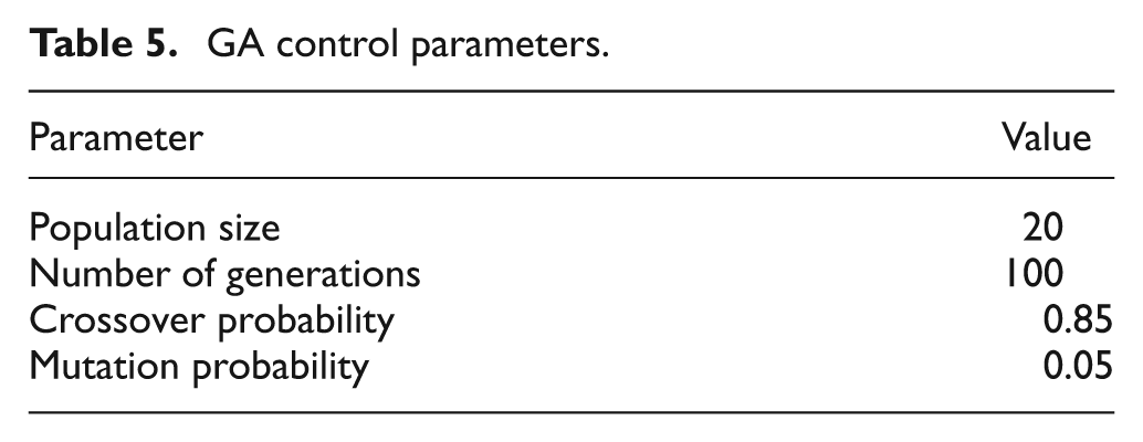
GA parameters

In this work, real coding of variables is used for the coding of the GA. Since three parameters (LA, MC, n _h ) are optimized, the chromosome has a string length of 3. Real coding of variables is followed. Intermediate operator for crossover and incremental operator for mutation ²⁰ are employed. Table 5 shows the other GA parameters used.

Table 5.

GA control parameters.

Parameter	Value
Population size	20
Number of generations	100
Crossover probability	0.85
Mutation probability	0.05

Analysis of results

Optimal network parameters

Figure 11 shows the screenshot of the learning performance of the network as taken from MATLAB. Initially the difference between the goal and the actual values is very large. This gap indicates the degree of lack of accuracy between the inputs to the ANN and how the ANN has understood the same. It can be seen that as the epochs increase, the difference between the goal and the actual error present during learning gets narrow and the actual training error meets the goal at 3971 epochs.

Figure 11.

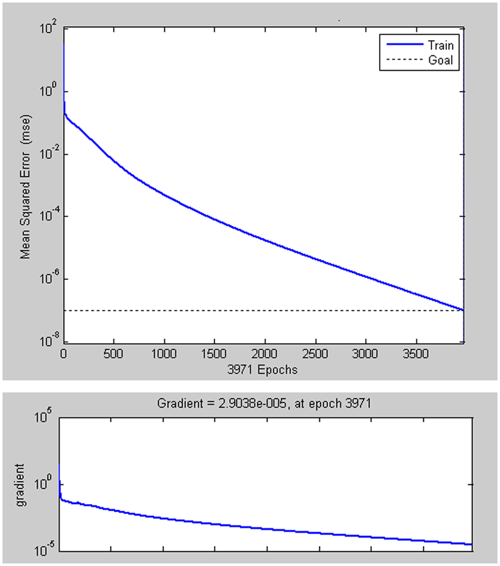
Learning performance of the ANN: (a) performance plot; (b) gradient plot.

It is also evident from the plot that the difference between the goal and the actual training error was nearly 100 and it ultimately gets reduced to 10⁻⁷. This shows that, had the ANN parameters not been optimized, it would have resulted in a large learning error. Since the accuracy of learning has a bearing on the generalization capability of the ANN, error in learning leads to an error in generalization. As a result, the WDM predicted by the network will also be flawed. This underscores the importance of optimizing the ANN parameters.

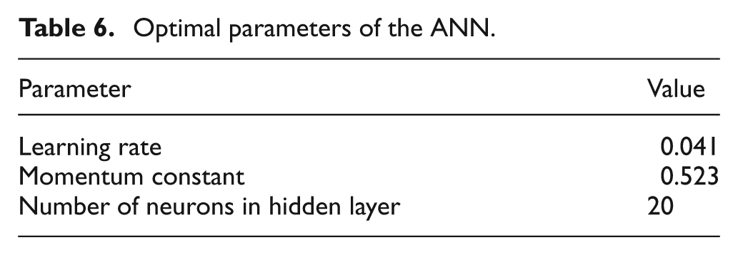
By achieving the set goal, it is proved that the network has a good learning capability. The optimal parameters pertaining to this result, as determined by the GA, are given in Table 6.

Table 6.

Optimal parameters of the ANN.

Parameter	Value
Learning rate	0.041
Momentum constant	0.523
Number of neurons in hidden layer	20

Generalization performance of the ANN

To study its generalization capability, the ANN was fed with the coordinate data of 20 different layouts. It can be noted that the WDM for these 20 layouts are also obtained experimentally. Now the values of the WDM that would be predicted by the ANN for these layouts are compared with the experimentally obtained values. Any difference between these two values is termed the generalization error and the same is quantified using a measure MARE, as explained in ‘Modeling of the ANN’. The relevant values for the 20 datasets are given in Table 7 and depicted in Figure 12. It can be seen that the difference between target and predicted values is very small. Figure 13 shows the ARE in percentage terms. It is seen that the maximum ARE is 9.71% and the MARE is found to be 0.03537.

Table 7.

Generalization performance of the ANN.

Dataset	WDM (µm)		ARE	ARE (%)
	Target	Predicted
1	12.36	11.80	0.045	4.53
2	11.78	10.64	0.097	9.71
3	11.86	12.55	0.059	5.85
4	10.36	10.05	0.030	2.99
5	17.41	16.99	0.024	2.41
6	11.71	10.92	0.067	6.68
7	15.39	15.27	0.008	0.78
8	16.51	16.98	0.029	2.86
9	12.98	13.21	0.018	1.78
10	11.03	10.98	0.005	0.48
11	14.25	14.83	0.041	4.07
12	13.78	12.64	0.083	8.27
13	10.91	11.05	0.013	1.28
14	14.56	13.84	0.049	4.95
15	15.05	15.58	0.035	3.52
16	17.20	17.01	0.011	1.10
17	17.84	18.06	0.012	1.23
18	11.65	11.34	0.027	2.66
19	13.02	13.50	0.037	3.69
20	18.08	17.63	0.025	2.49
MARE			0.035667955

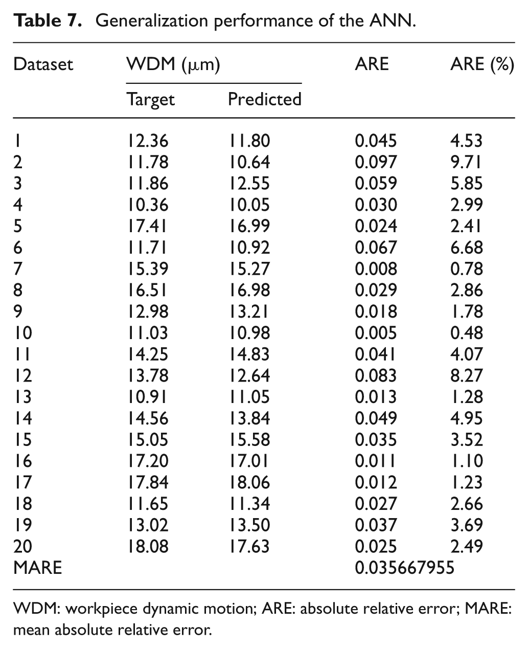
WDM: workpiece dynamic motion; ARE: absolute relative error; MARE: mean absolute relative error.

Figure 12.

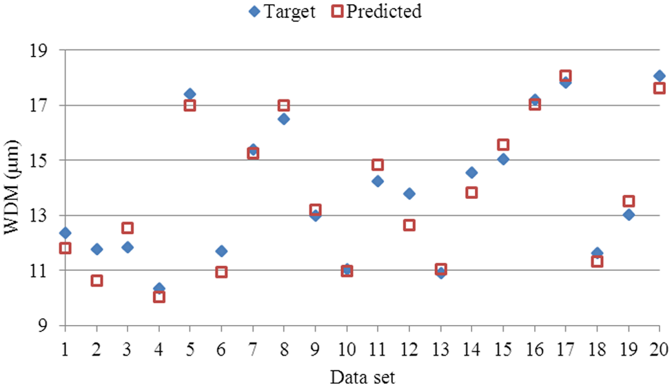
Target and predicted WDM in generalization.

Figure 13.

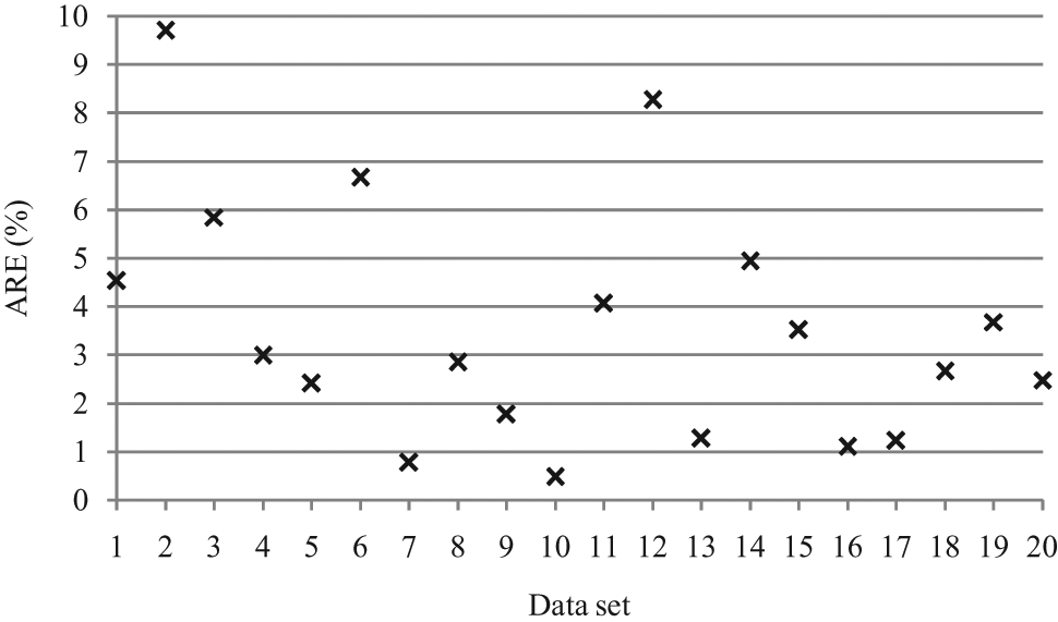
Percentage of ARE in generalization.

From Table 7 it can be noted that the difference between the target and predicted values for individual datasets differs. In some cases both data are almost the same, whereas in some other cases a difference exists. Going by individual pairs of data could lead to a prejudiced conclusion about the ANN performance. Because of the same reason, a parameter such as the MARE was necessary, which can collectively rate the accuracy of ANN prediction rather than on the basis of individual data.

Effect on machining tolerance

Now that the magnitude of the WDM is known, it can be assessed against the machining tolerance of 0.05 mm provided on the workpiece (Figure 2). For example, for layout 1 in Table 7, the ANN predicted value of the WDM is 11.8 µm (0.0118 mm). This means that, this particular layout has a ‘window’ of 0.0382 mm that can be shared by the other sources of error in the WFS. These sources include, but are not restricted to, those mentioned in the introduction.

On the other hand, if the predicted WDM exceeds 0.05 mm, this layout can straightaway be rejected. This is because, with a single source alone resulting in 0.05 mm machining error, the effect of one or more components owing to the above-mentioned sources would only cause the overall machining error to exceed 0.05 mm. This leads to non-conformance to the tolerance requirements.

Conclusions

This article presented a novel approach of predicting WDM using an optimized ANN. Using a modular fixture set-up, different layouts were obtained and the WDM was computed at the datum points experimentally. An ANN was trained using this data. Learning rate, momentum constant and number of neurons in the hidden layer of the ANN were identified as critical parameters, and these were optimized so as to achieve a better prediction efficiency of the network. The performance measure of the ANN showed that the network has good learning and generalization capabilities. With the ANN proved to be efficient, it can now be used for the evaluation of WDM for any required layout. This, in turn, can serve as an economical and efficient method for fixture layout optimization.