Sage Journals: Discover world-class research

Abstract

A novel surface finishing method using an improved ball end magnetorheological finishing tool was developed for nanofinishing of flat, as well as three-dimensional workpiece surfaces. An improved magnetorheological finishing tool is the main part of the present finishing process, which has been made up of the central rotating core and stationary electromagnet coil integrated with a copper cooling coil. A magnetically generated ball end finishing spot of magnetorheological polishing fluid was used as a finishing segment at the tip surface of the rotating core. In this research, detailed study through statistical design of the experiments was conducted for nanofinishing of ferromagnetic workpieces by the proposed ball end magnetorheological finishing process. Response surface methodology has been used to plan and analyze the effect of rotational speed of the tool core, magnetizing current and working gap on percentage change in surface roughness. The experimental results were discussed and the best finishing conditions were identified within the experimental range of variables. Analysis of experimental data showed that the percentage change in surface roughness was highly influenced by the working gap, followed by magnetizing current and rotational speed of the tool core. The best surface finish obtained on the ferromagnetic workpieces was as low as 27.6 nm from the initial value of 142.9 nm in 30 min of finishing time. In order to study the finished surface morphology, scanning electron microscopy and atomic force microscopy were also conducted.

Keywords

Magnetorheological finishing ball end magnetorheological finishing tool magnetorheological polishing fluid response surface methodology

Introduction

Surface finish has a higher influence on functional properties, such as wear resistance and power loss, owing to friction on most engineering components. Finishing processes also need to meet the requirements of high surface finish, accuracy, and minimum surface defects.¹ In last few decades, to overcome the limitations of traditional finishing processes and precise control of finishing forces during operation, a number of magnetic field-assisted finishing techniques utilizing smart magnetorheological (MR) fluid have been developed. MR finishing (MRF) has been described as an advanced polishing technique that can finish optics without propagating the subsurface damage layer.² The normal force on an individual abrasive particle in MRF is relatively small compared with conventional polishing techniques, and therefore, material removal in MRF is governed by shear stress rather than the hydrodynamic pressure.³ Shorey⁴ calculated that the normal force acting on a single abrasive particle within the MR fluid ribbon is approximately 1 × 10⁻⁷ N. This is several orders of magnitude smaller than that for conventional polishing, 5 – 200 × 10⁻³ N.⁵ MR fluids are the key element of MRF technology.⁶ MRF is used for precision finishing of concave, convex, flat, and aspherical optical components.⁷ Kim et al.⁸ proposed a MRF process for three-dimensional (3D) silicon microchannel finishing using the flow of the stiffened MR fluid. The rotational axis of the magnet is vertically set up to prevent hydrodynamic pressure between the magnet and specimen. The existing MRF is not proper for micro-channel finishing because of severe hydrodynamic pressure (up to 100 KPa) between the parts and the rotating large wheel destroys the channel structures.

In recent years, several researchers have reported on developments of the MRF process. Seok et al.⁹ proposed a MRF process for fabrication of curved surfaces on silicon-based micro-structures in which the edge effect is actively utilized. Cheng et al.¹⁰ presented polishing of optical aspheric components using a two-axis wheel-shaped tool supporting dual magnetic fields. Jacobs¹¹ reported that MRF can be used for difficult-to-finish optical materials, like soft polymer polymethyl methacrylate, microstructured polycrystalline zinc sulfide, and water soluble single-crystal potassium dehydrogenate phosphate, by systematic alteration of MR fluid chemistry. Miao et al.¹² studied the effect of volume fraction of nanodiamond abrasive, magnetic field, wheel speed, and penetration depth on material removal for borosilicate glass. Also, the current authors have already reported the existing ball end MRF (BEMRF) process,¹³ where the finishing tool was rotated as a whole during the finishing operation, which lead to the limitation of stable and longer duration of finishing applications. In this design there was no provision for cooling the electromagnet coil owing to its rotation. Process capabilities in finishing of ferromagnetic and non-ferromagnetic materials have already been demonstrated and reported.¹³

In the present MRF process, an improved BEMRF tool has been used, which comprises of a central rotating core, stationary electromagnet coil, and further copper cooling coils wrapped over the outer surface of the stationary electromagnet coil for continuous cooling. The cooling medium is supplied by a low temperature bath. A magnetically generated ball end finishing spot of MR polishing (MRP) fluid at the tip surface of the rotating core is used as a finishing segment to finish the workpiece surfaces. The flow of MRP fluid at the tip of the rotating core is not continuous. It means, whenever MRP fluid is required to be conditioned after a certain period of finishing operation only then was it made to flow to the tip surface of the rotating core through a peristaltic pump. Otherwise, an already formed ball end finishing spot of MRP fluid is used continuously for the finishing operation. The complete set-up and process can be visualized similar to a three-axis vertical computer numerically controlled (CNC) machine with a ball end milling cutter.

The BEMRF tool has comparatively less limitations on finishing of different workpiece surfaces, as compared with regular MRF. The finishing spot of MRP fluid formed at the tip surface of the central rotating core can be easily made reachable for the different 3D surface profiles. The vertical tapered tool tip, with finishing spot of MRP fluid, can be moved and performed finishing with the help of a computer controlled program over different kinds of surfaces in a workpiece, such as projections at different angles or in-depth pocket profiles; whereas finishing of these surfaces in the workpiece are likely to be inaccessible by a regular MRF process owing to rotating wheel size or mechanical interferences. MR jet finishing was developed to finish the internal surface of a steep concave and spherical dome, where the jet was impinged on the workpiece surface from the bottom and the workpiece surface was rotated relative to the MR jet.¹⁴ In this process, the relative movement of different 3D complex workpiece surfaces, with respect to the MR jet, may have challenged the task. The newly developed finishing process can be found in more industrial applications in the area of MRF processes.

The mechanism of BEMRF is shown in Figure 1. The pressurized MRP fluid enters from the top end of the central rotating core. As soon as it reaches the tip surface of the tool the electromagnet is switched ON. A ball end shape of the finishing spot, with semi-solid structure, is formed at the tip surface of the rotating core (Figure 2(b)). When the magnet is switched OFF, the ball end finishing spot of the MRP fluid breaks down and behaves like a paste-type of viscous fluid (Figure 2(c)). The finishing action and feed direction on workpiece is shown in Figure 2(a). The material removed from the workpiece surface by silicon carbide abrasives depends on the bonding forces between the carbonyl iron particles in the finishing spot of the MRP fluid. The finishing force F_F is developed by the finishing spot of the MRP fluid on the workpiece surface. This is a resultant of normal force F_n along the direction of magnetic lines of forces and shear force F_t along the direction of the core rotation (Figure 1).

Figure 1.

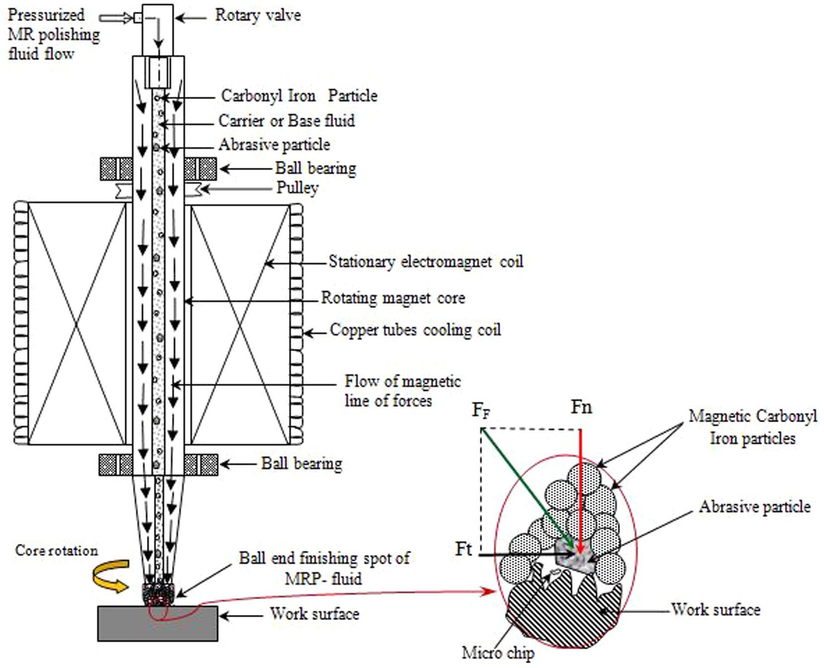
Mechanism of the BEMRF process.

Figure 2.

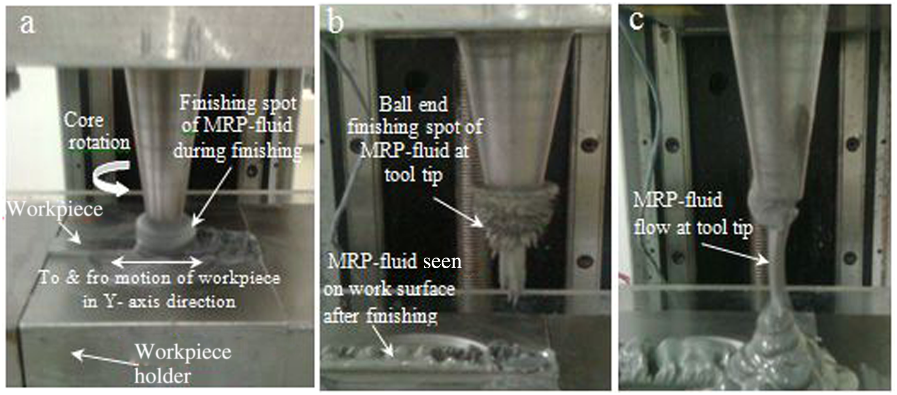
MR polishing fluid at the tip surface of MR finishing tool: (a) during finishing on workpiece surface; (b) after finishing, where the electromagnet is still kept ON; and (c) when the magnet is OFF.

A schematic and photograph of the BEMRF set-up, as per the developed design, is shown in Figures 3 and 4. The improved MRF tool is fixed on the vertical Z-side of the XYZ movement table. A servo motor is used to control the rotational speed of the central rotating core. The X–Y direction stepper motors are used to control the horizontal linear feed rate of the workpiece and the Z-direction stepper is used to control the vertical linear feed rate of MRF tool. All motors are driven by computer controlled drives and controllers. A regulated d.c. power supply is used to control the magnetizing current of the electromagnet coil. A PT100 resistance temperature detector (RTD), inserted in to the electromagnet coil and variation of coil temperature during finishing, is recorded through a digital temperature display. The electromagnet coil temperature is monitored and controlled by a constant low temperature bath.

Figure 3.

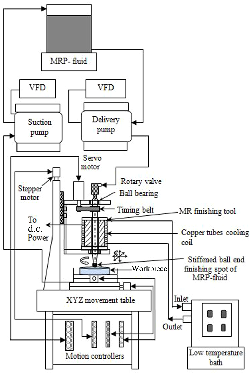
Schematic of the BEMRF experimental set-up.

Figure 4.

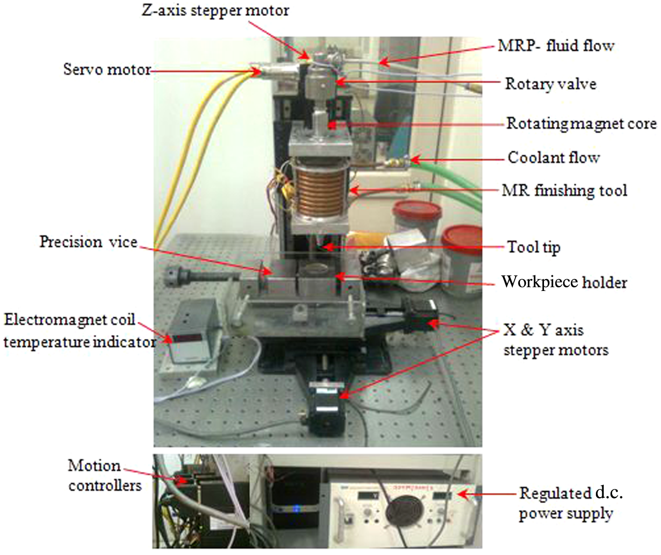
Photograph of the BEMRF experimental set-up.

The MRP fluid delivery system is shown in Figure 5. The MRP fluid is prepared in a funnel-shaped reservoir with the help of d.c. speed controlled stirrer. A peristaltic pump has been used for supplying MRP fluid through a fluid flow passage up to the tip surface of the rotating core from the reservoir. The speed of the peristaltic pump is controlled and monitored by an a.c. variable frequency drive (VFD).

Figure 5.

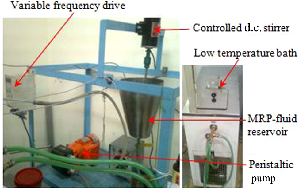
Photograph of a MRP fluid circulation system.

BEMRF process variables

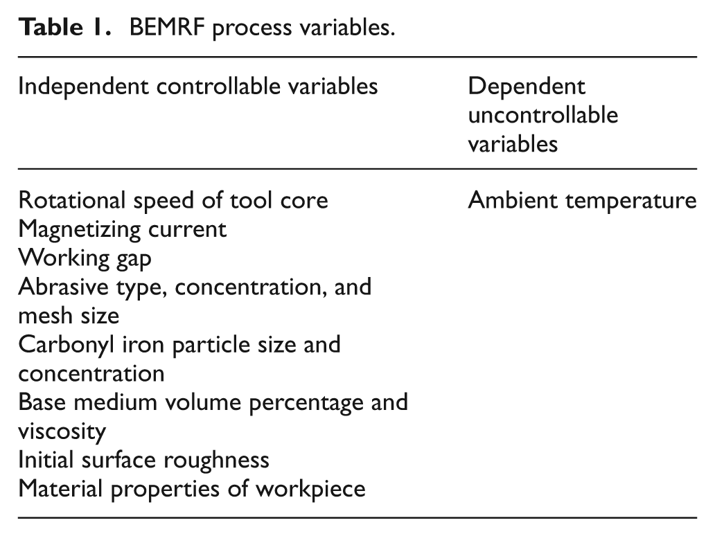
BEMRF process is a comparatively new finishing process and there is a lack of experimental data available in literature on it. Therefore, based on the similarity of the process with MRF, the controllable and uncontrollable variables are identified and listed in Table 1. Out of the listed variables, the independent controllable variables are selected for parametric study as described below.

Table 1.

BEMRF process variables.

Independent controllable variables	Dependent uncontrollable variables
Rotational speed of tool core	Ambient temperature
Magnetizing current
Working gap
Abrasive type, concentration, and mesh size
Carbonyl iron particle size and concentration
Base medium volume percentage and viscosity
Initial surface roughness
Material properties of workpiece

Rotational speed of tool core (N)

Rotational speeds of the tool core, with finishing spot of MRP fluid on the workpiece surface, removes the peaks from the surface and finishes the surface where the tool tip can reach. The removal of material, in the form of µ-chips, can be found owing to shear force during rotation of the central core with a finishing spot of MRP fluid. Experiments were conducted from 332 to 668 r/min, depending on the levels of statistical design. The range of these values was chosen on the basis of preliminary experimentation.

Magnetizing current (I)

The change in rheological properties of the ball end finishing spot of MRP fluid at the tip of the rotating core depends on the strength of magnetic flux density, which in turn depends on the supply of the magnetizing current to the electromagnet coil. The strength of the finishing spot of MRP fluid at the tip of the rotating core can be controlled by controlling the supply of d.c. to the electromagnet coil. The material removed from the workpiece surface by abrasive grains depends on the bonding forces between carbonyl iron particles in the finishing spot of MRP fluid. Experiments were conducted by varying the magnetizing current 2.3 to 5.7 A. These magnetizing current values were selected in the range of low to high, as per the prescribed design of the electromagnet.

Working gap (D)

The working gap is the distance between the tip surface of the tool and workpiece surface. The strength of the finishing spot of MRP fluid at the tip surface of the rotating core can be controlled by varying the working gap while the d.c. supply to the electromagnet coil is kept constant. It mean that, when the tip surface of the tool is kept closer to the workpiece surface for a constant supply of current, the magnetic field at the tip surface of the rotating core increases, making the finishing spot of MRP-fluid more stiffen which results more removal of peaks from workpiece surface. Similarly, when the tip surface of the rotating core is kept comparatively away from the workpiece surface for the same supplying current, the magnetic field at the tool tip surface decreases, making the finishing spot of the MRP fluid less stiff. In this case, less removal of peaks from the workpiece surface can be found. Hence, the finishing forces exerted by the finishing spot of the MRP fluid on the workpiece surface can be found to be higher at the lower working gap and relatively less at the higher working gap for supplying the same current. The experiments were conducted with a working gap range of 0.66–2.34 mm. These values were chosen on the basis of magnetostatic simulation where it has been checked the magnetic flux density on various working gaps filled with a MRP fluid layer using Maxwell student version finite element analysis software.

Design of experiments

Designed experiments were used to systematically investigate the influence of process variables on the surface finish improvement. Experiments were performed on a BEMRF experimental set-up designed and developed by the authors as shown in Figures 3 and 4. Since flat surfaces facilitate easy measurement and observations under a scanning electron microscopy (SEM) and atomic force microscopy (AFM), for a detailed study the experiments were performed on flat workpieces of dimension 70 × 10 × 4 mm, which was obtained after surface grinding. The initial surface roughness R_a was approximate in the range 0.0906–0.1651 µm. The initial surface roughness of the ground workpieces is not equal for all the workpieces, therefore, this variation was taken into account by considering the ratio of change in surface roughness to the initial roughness as a response and is given equation (1). A workpiece holder of die steel was made by milling a rectangular slot of the workpiece dimension. The workpiece was kept in a rectangular slot of the workpiece holder and precision vice held the workpiece holder tightly along with workpiece on X–Y movement linear slides driven by computer controlled stepper motors. Since the size of tool tip diameter and width of the workpiece were same (10 mm), only the reciprocating motion of the workpiece through the Y-axis stepper motor was given for complete finishing of work surface (Figure 2(a)).

Response surface methodology (RSM) is a collection of statistical and mathematical methods that are useful for modeling and analyzing engineering problems. RSM also quantifies the relationship between the controllable input parameters and the obtained response surfaces. In full factorial experiment, the responses are measured at all combinations of the factor levels. The combination of factor levels represent the conditions at which experiments will be conducted and responses will be measured.¹⁵ Two level, full factorial designs with six central runs and six axial runs leading to the central composite rotatable design were used to conduct the experiments. To know the significance of the regression equation in explaining the relationship between surface finish improvement and controllable process parameters, ‘F’ test from the analysis of variance (ANOVA) was conducted. The effects of three process variables were investigated on percentage change in surface roughness (%ΔR_a) using a full factorial design. The material removal found from the initial experiments was too small (micrograms) to measure by the normal precision measuring balance, hence it was not considered as a response.

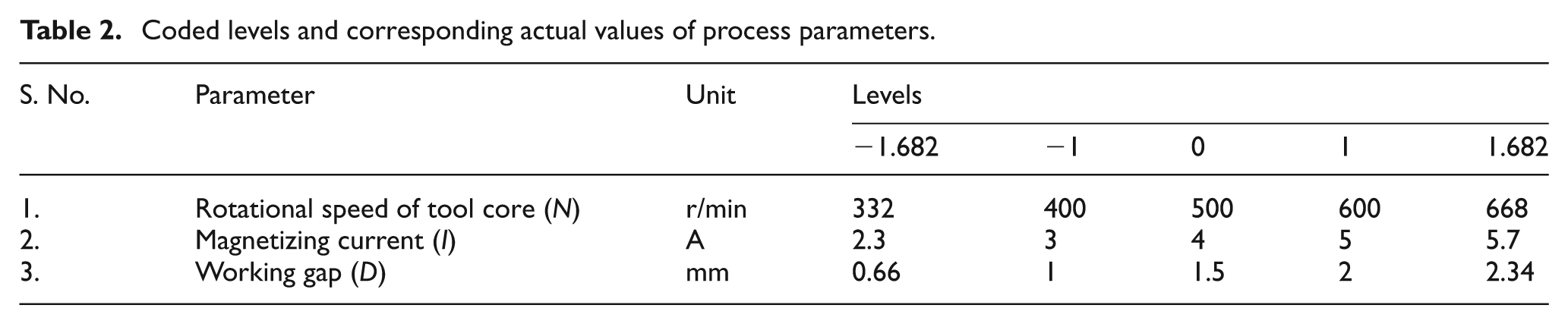
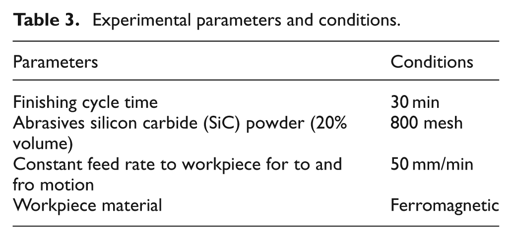
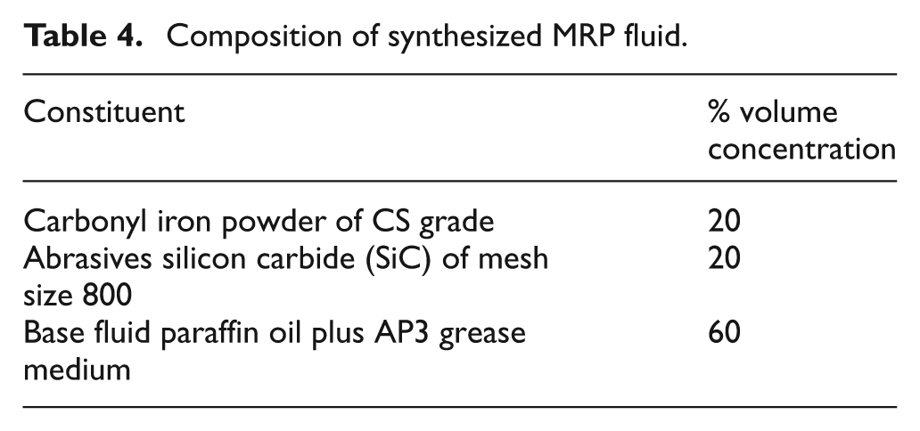
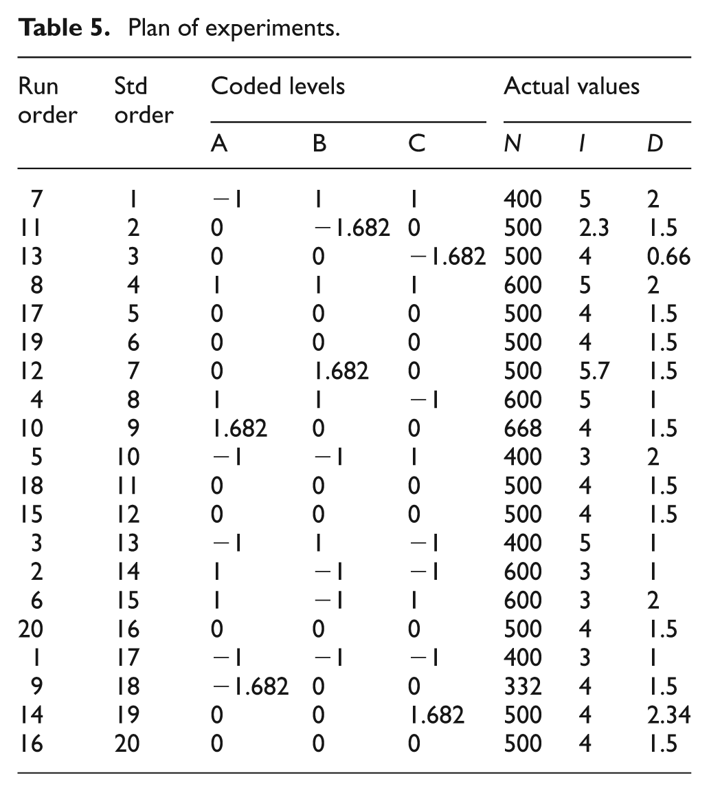
Table 2 lists the coded levels and actual values of different parameters used in BEMRF of the ferromagnetic workpiece. The other experimental conditions are listed in Table 3. MRP fluid was prepared by mixing the compositions as per the percentage volume concentration given in Table 4. Experiments were conducted on the ferromagnetic workpiece in random order, as per the plan of experiments given in Table 5.

Table 2.

Coded levels and corresponding actual values of process parameters.

S. No.	Parameter	Unit	Levels
			−1.682	−1	0	1	1.682
1.	Rotational speed of tool core (N)	r/min	332	400	500	600	668
2.	Magnetizing current (I)	A	2.3	3	4	5	5.7
3.	Working gap (D)	mm	0.66	1	1.5	2	2.34

Table 3.

Experimental parameters and conditions.

Parameters	Conditions
Finishing cycle time	30 min
Abrasives silicon carbide (SiC) powder (20% volume)	800 mesh
Constant feed rate to workpiece for to and fro motion	50 mm/min
Workpiece material	Ferromagnetic

Table 4.

Composition of synthesized MRP fluid.

Constituent	% volume concentration
Carbonyl iron powder of CS grade	20
Abrasives silicon carbide (SiC) of mesh size 800	20
Base fluid paraffin oil plus AP3 grease medium	60

Table 5.

Plan of experiments.

Run order	Std order	Coded levels			Actual values
		A	B	C	N	I	D
7	1	−1	1	1	400	5	2
11	2	0	−1.682	0	500	2.3	1.5
13	3	0	0	−1.682	500	4	0.66
8	4	1	1	1	600	5	2
17	5	0	0	0	500	4	1.5
19	6	0	0	0	500	4	1.5
12	7	0	1.682	0	500	5.7	1.5
4	8	1	1	−1	600	5	1
10	9	1.682	0	0	668	4	1.5
5	10	−1	−1	1	400	3	2
18	11	0	0	0	500	4	1.5
15	12	0	0	0	500	4	1.5
3	13	−1	1	−1	400	5	1
2	14	1	−1	−1	600	3	1
6	15	1	−1	1	600	3	2
20	16	0	0	0	500	4	1.5
1	17	−1	−1	−1	400	3	1
9	18	−1.682	0	0	332	4	1.5
14	19	0	0	1.682	500	4	2.34
16	20	0	0	0	500	4	1.5

Response surface regression analysis

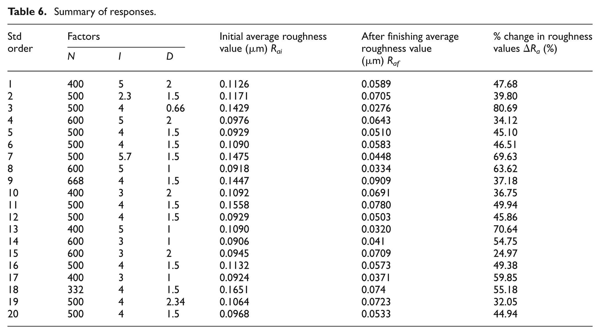
The responses in terms of absolute value of surface roughness (R_a) and percentage change in roughness value (%ΔR_a) are presented in Table 6. The response surface for percentage change in R_a value is analyzed.

Table 6.

Summary of responses.

Std order	Factors			Initial average roughness value (µm) R_ai	After finishing average roughness value (µm) R_af	% change in roughness values ΔR_a (%)
Std order	N	I	D	Initial average roughness value (µm) R_ai	After finishing average roughness value (µm) R_af	% change in roughness values ΔR_a (%)
1	400	5	2	0.1126	0.0589	47.68
2	500	2.3	1.5	0.1171	0.0705	39.80
3	500	4	0.66	0.1429	0.0276	80.69
4	600	5	2	0.0976	0.0643	34.12
5	500	4	1.5	0.0929	0.0510	45.10
6	500	4	1.5	0.1090	0.0583	46.51
7	500	5.7	1.5	0.1475	0.0448	69.63
8	600	5	1	0.0918	0.0334	63.62
9	668	4	1.5	0.1447	0.0909	37.18
10	400	3	2	0.1092	0.0691	36.75
11	500	4	1.5	0.1558	0.0780	49.94
12	500	4	1.5	0.0929	0.0503	45.86
13	400	5	1	0.1090	0.0320	70.64
14	600	3	1	0.0906	0.041	54.75
15	600	3	2	0.0945	0.0709	24.97
16	500	4	1.5	0.1132	0.0573	49.38
17	400	3	1	0.0924	0.0371	59.85
18	332	4	1.5	0.1651	0.074	55.18
19	500	4	2.34	0.1064	0.0723	32.05
20	500	4	1.5	0.0968	0.0533	44.94

Δ R_{a} (%) = [(R_{a i} - R_{a f}) / R_{a i}] \times 100

(1)

The sequential model sum of squares was calculated to select the highest order polynomial where the additional terms are significant and the model is not aliased. Table 7 of sequential model sum of squares shows how terms of increasing complexity contribute to the total model. The significance of adding quadratic terms to two factor interactions and linear terms is highest, as it has a high F-value and least p-value, suggesting its suitability. Lack of fit for all possible models was calculated and is presented in Table 8. For the selected quadratic model, the lack of fit is insignificant.

Table 7.

Sequential model sum of squares.

Source	Sum of squares	DOF	Mean square	F-value	p-value Prob > F	Remark
Mean versus total	48870.45	1	48870.45
Linear versus mean	3492.27	3	1164.0958.95	<0.0001
2FI versus linear	23.58	3	7.86	0.35	0.7902
Quadratic versus 2FI^*	167.38	3	55.79	4.46	0.0310	Suggested
Cubic versus quadratic	57.46	4	14.36	1.28	0.3754	Aliased
Residual	67.55	6	11.26
Total	52678.68	20	2633.93

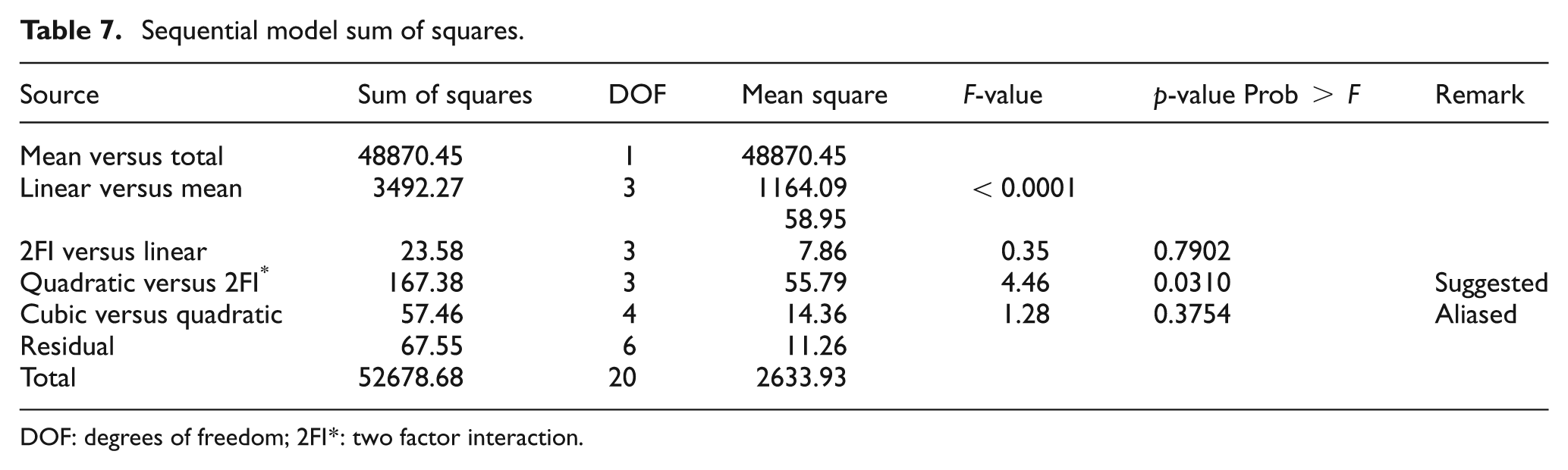
DOF: degrees of freedom; 2FI*: two factor interaction.

Table 8.

Lack of fit tests.

Source	Sum of squares	DOF	Mean square	F-value	p-value Prob > F	Remark
Linear	292.27	11	26.57	5.61	0.0349
2FI	268.69	8	33.59	7.09	0.0226
Quadratic	101.31	5	20.26	4.28	0.0683	Suggested
Cubic	43.86	1	43.86	9.26	0.0287	Aliased
Pure Error	23.69	5	4.74

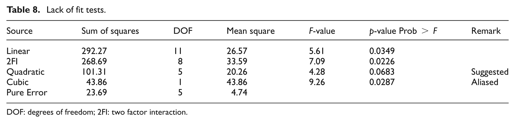
DOF: degrees of freedom; 2FI: two factor interaction.

On the basis of Tables 7 and 8, a quadratic model was selected. Initially, all the terms such as N, I, D, NI, ND, ID, N², I² and D² were included in the response surface model. The ANOVA for this model is given in Table 9. The model F-value of 32.74 implies that the model is significant. There is only a 0.01% chance that this large ‘Model F-Value’ could occur owing to noise. If the values of ‘Prob > F’ is less than 0.05, then it indicates that the model is significant. The significant level (0.05) for a given hypothesis test is a value, for which a p–value is less than or equal to α, is considered statistically significant. Typical value for α are 0.1, 0.05, and 0.01. These values correspond to the probability of observing such an extreme value by chance. The significance level α corresponds to the value for which one can choose to reject or accept the null hypothesis H₀. The probability that null hypothesis is true is α. In decision theory, this is known as a Type I error. The probability of a Type I error is equal to the significance level α. To minimize the probability of a Type I error, the significance level is generally chosen to be small.

Table 9.

ANOVA for percentage change in R_a.

Source	Sum of squares	DOF	Mean square	F-value	p-value Prob > F	Remark
Model	3683.23	9	409.25	32.74	<0.0001	Significant
N	335.92	1	335.92	26.87	0.0004
I	591.90	1	591.90	47.35	<0.0001
D	2564.45	1	2564.45	205.15	<0.0001
NI	1.71	1	1.71	0.14	0.7191
ND	21.85	1	21.85	1.75	0.2156
ID	0.022	1	0.022	1.764E-003	0.9673
N ²	16.07	1	16.07	1.29	0.2833
I ²	55.45	1	55.45	4.44	0.0614
D ²	93.47	1	93.47	7.48	0.0210
Residual	125.00	10	12.50
Lack of fit	101.31	5	20.26	4.28	0.0683	Not significant
Pure error	23.69	5	4.74

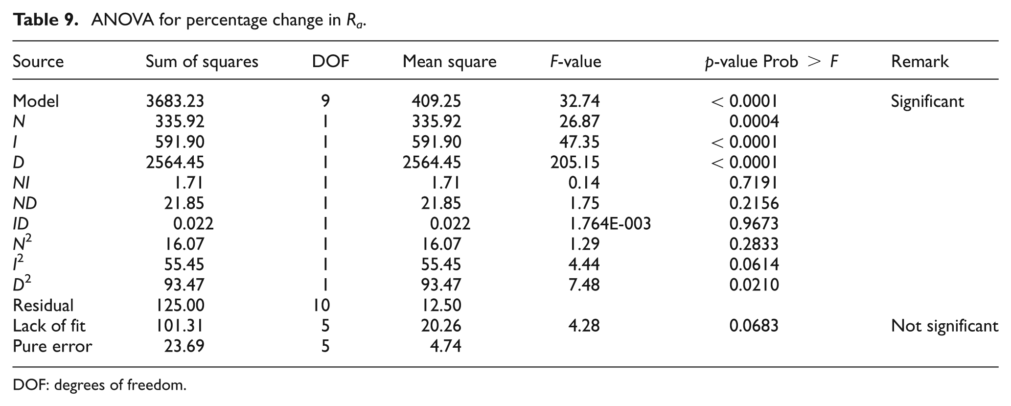
DOF: degrees of freedom.

In the present study the significance level is taken as α = 0.05. In this case N, I, D, and D² are significant terms. p–values greater than 0.05 indicate that terms are not significant. If there are many insignificant terms, then the model reduction by removing insignificant terms may improve the model. The lack of fit is the variation of data around the fitted model. The ‘lack of fit F-value’ of 4.28 implies there is a 6.83% chance that this large ‘lack of fit F-value’ could occur owing to noise.

Other ANOVA parameters are given in Table 10. The ‘predicted R²’, is a measure of how good the model predicts a response value. The adjusted R² and predicted R² should be within approximately 0.20 of each other.¹⁶ The predicted R² of 0.7895 is within a reasonable distance to the adjusted R² of 0.9376. ‘Adequate precision’ measures the signal to noise ratio. A ratio greater than 4 is desirable. In the above model, this ratio of 21.314 indicates an adequate signal. This model can be used to navigate the design space.

Table 10.

Other ANOVA parameters.

Std. Dev.	3.54	R ²	0.9672
Mean	49.43	Adj R²	0.9376
C.V. %	7.15	Pred R²	0.7895
PRESS	801.56	Adeq Precision	21.314

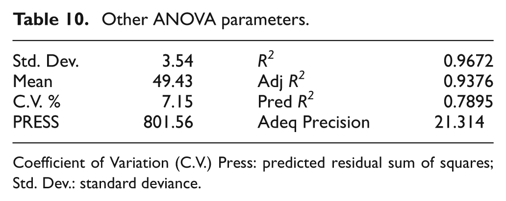
Coefficient of Variation (C.V.) Press: predicted residual sum of squares; Std. Dev.: standard deviance

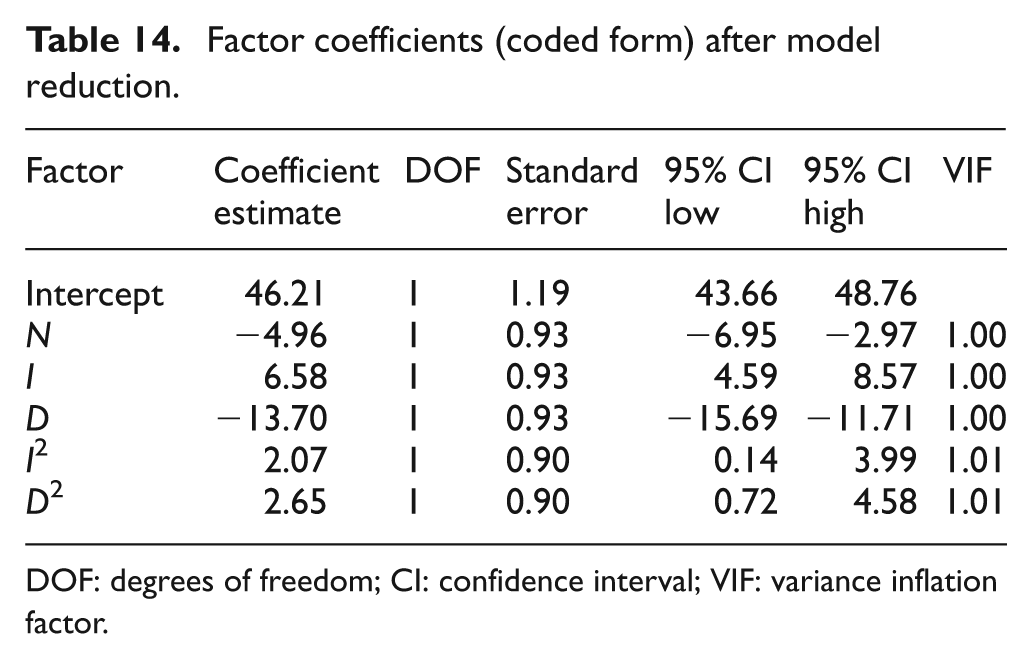
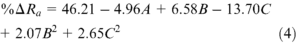
The 95% confidence interval (CI) high and low values are the upper and lower bound of the 95% CI that surrounds the coefficient estimate for the factor. The values in Table 11 represent the range that the true coefficient should be found in 95% of the time. If this range spans 0 (one limit is positive and the other negative) then the coefficient of 0 could be true, indicating the factor has no effect. The variance inflation factor (VIF) measures how much the variance of the model is inflated by the lack of orthogonality in the design. If the factor is orthogonal to all other factors in the model, the VIF is one. Values greater than 10 indicate that the factors are too correlated together (they are not independent). Depending on the coefficients calculated in Table 11, the final equation in terms of coded factors is given as

Table 11.

Factor coefficients (coded form).

Factor	Coefficient estimate	DOF	Standard error	95% CI low	95% CI high	VIF
Intercept	47.07	1	1.44	43.86	50.29
N	−4.96	1	0.96	−7.09	−2.83	1.00
I	6.58	1	0.96	4.45	8.72	1.00
D	−13.70	1	0.96	−15.83	−11.57	1.00
NI	−0.46	1	1.25	−3.25	2.32	1.00
ND	−1.65	1	1.25	−4.44	1.13	1.00
ID	0.053	1	1.25	−2.73	2.84	1.00
N ²	−1.06	1	0.93	−3.13	1.02	1.02
I ²	1.96	1	0.93	−0.11	4.04	1.02
D ²	2.55	1	0.93	0.47	4.62	1.02

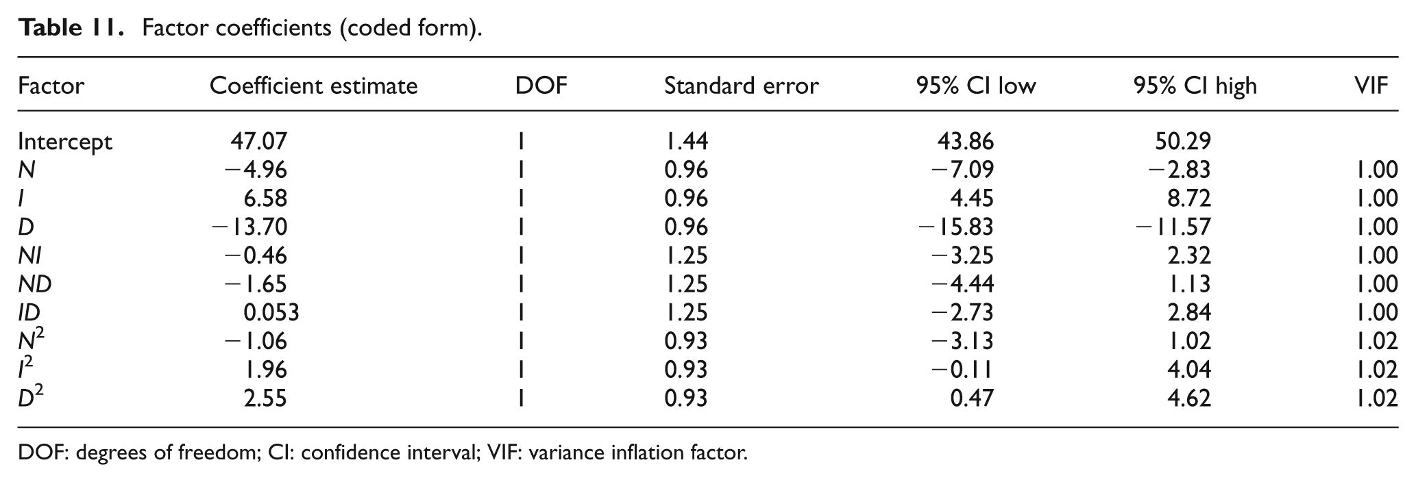
DOF: degrees of freedom; CI: confidence interval; VIF: variance inflation factor.

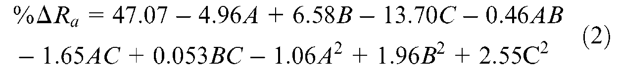
\begin{array}{l} % Δ R_{a} = 47.07 - 4.96 A + 6.58 B - 13.70 C - 0.46 A B \\ - 1.65 A C + 0.053 B C - 1.06 A^{2} + 1.96 B^{2} + 2 . {55C}^{2} \end{array}

(2)

Final equation in terms of actual factors is given as

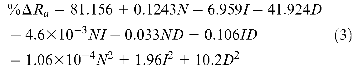
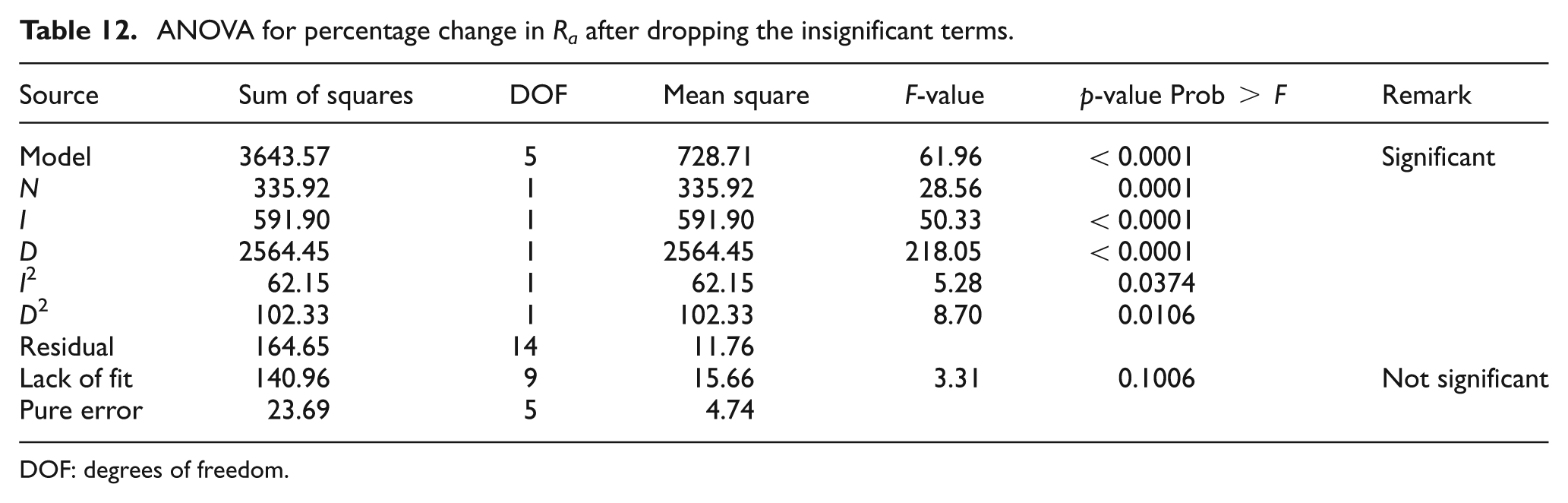
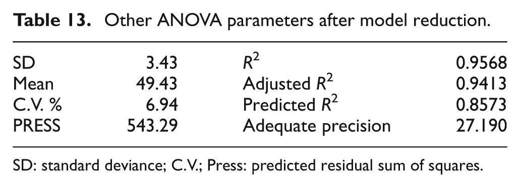
\begin{array}{l} % Δ R_{a} = 81.156 + 0.1243 N - 6.959 I - 41.924 D \\ - 4.6 \times 1 0^{- 3} N I - 0.033 N D + 0.106 I D \\ - 1.06 \times 1 0^{- 4} N^{2} + 1.96 I^{2} + 10.2 D^{2} \end{array}

(3)

A p- value greater than 0.05 indicates that the model terms are not significant. There are five insignificant model terms (Table 9), therefore, the reduction of the model by dropping insignificant terms may improve the model. The ANOVA, after dropping the insignificant terms, is presented in Tables 12 and 13. The model F-value of 61.96 implies the model is significant. There is only a 0.01% chance that this large ‘model F-value’ could occur owing to noise. Values of ‘prob > F’ less than 0.05 indicate that the model terms are significant. In this case N, I, D, I², D² are significant model terms. The ‘predicted R²’ of 0.8573 is in reasonable agreement with the ‘adjusted R^2’ of 0.9413. The adequate precision value measures the signal to noise ratio. A ratio greater than 4 is desirable. The ratio of 27.190 indicates an adequate signal. Factor coefficients (coded form) after model reduction, given in Table 14, represent the range that the true coefficient should be found 95% of the time.

Table 12.

ANOVA for percentage change in R_a after dropping the insignificant terms.

Source	Sum of squares	DOF	Mean square	F-value	p-value Prob > F	Remark
Model	3643.57	5	728.71	61.96	<0.0001	Significant
N	335.92	1	335.92	28.56	0.0001
I	591.90	1	591.90	50.33	<0.0001
D	2564.45	1	2564.45	218.05	<0.0001
I ²	62.15	1	62.15	5.28	0.0374
D ²	102.33	1	102.33	8.70	0.0106
Residual	164.65	14	11.76
Lack of fit	140.96	9	15.66	3.31	0.1006	Not significant
Pure error	23.69	5	4.74

DOF: degrees of freedom.

Table 13.

Other ANOVA parameters after model reduction.

SD	3.43	R ²	0.9568
Mean	49.43	Adjusted R²	0.9413
C.V. %	6.94	Predicted R²	0.8573
PRESS	543.29	Adequate precision	27.190

SD: standard deviance; C.V.; Press: predicted residual sum of squares

Table 14.

Factor coefficients (coded form) after model reduction.

Factor	Coefficient estimate	DOF	Standard error	95% CI low	95% CI high	VIF
Intercept	46.21	1	1.19	43.66	48.76
N	−4.96	1	0.93	−6.95	−2.97	1.00
I	6.58	1	0.93	4.59	8.57	1.00
D	−13.70	1	0.93	−15.69	−11.71	1.00
I ²	2.07	1	0.90	0.14	3.99	1.01
D ²	2.65	1	0.90	0.72	4.58	1.01

DOF: degrees of freedom; CI: confidence interval; VIF: variance inflation factor.

The final equation in terms of coded factors is

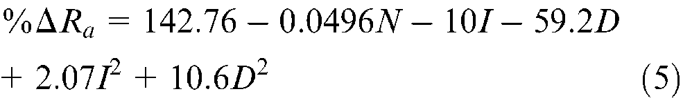
\begin{array}{l} % Δ R_{a} = 46.21 - 4.96 A + 6.58 B - 13.70 C \\ ​ + 2.07 B^{2} + 2.65 C^{2} \end{array}

(4)

The final equation in terms of actual factors is given as

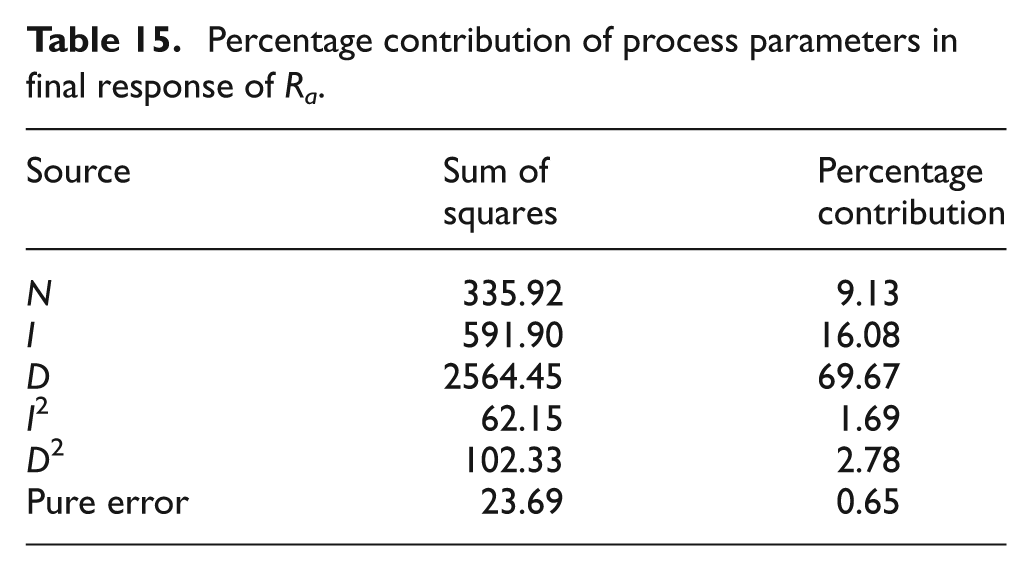
\begin{array}{l} % Δ R_{a} = 142.76 - 0.0496 N - 10 I - 59.2 D \\ + 2.07 I^{2} + 10.6 D^{2} \end{array}

(5)

Percentage contributions of process parameters on the improvement in surface roughness R_a are presented in Table 15.

Table 15.

Percentage contribution of process parameters in final response of R_a.

Source	Sum of squares	Percentage contribution
N	335.92	9.13
I	591.90	16.08
D	2564.45	69.67
I ²	62.15	1.69
D ²	102.33	2.78
Pure error	23.69	0.65

Results and discussion

Based on the results of the response surface model obtained after regression analysis, the results in terms of the effect of rotational speed of tool core, magnetizing current, and working gap on the percentage reduction of surface roughness have been observed and computed. No interaction effect is found to be significant in ANOVA, hence neglected. The effects of independent controllable variables in percentage change of R_a have been discussed as follows.

Effect of rotational speed of tool core

As seen in Figure 6, the percentage change in surface roughness reduces with an increase in rotational speed of the tool core. The increase in r/min of the central rotating core beyond the given position may reduce the percentage change in R_a value. This is because at higher rotational speeds the effect of centrifugal force acting on carbonyl iron particles at a given position begins to increase beyond the magnetic force of attraction exerted on these particles. Therefore, the magnetic normal force marginally decreases with an increase in speed. Owing to this, carbonyl iron particles are not able to hold abrasive particles strongly enough during finishing. The decrease in magnetic normal force can be partially caused by a scattering of the few abrasives from the working gap at a higher speed of the tool core. Since centrifugal force is proportional to the square of the rotating speed, when attempting to increase the percentage change in R_a value by increasing the rotational speed of tool core, the centrifugal force acting on carbonyl iron particles plays an adverse role for percentage change in the R_a value. Hence, magnetic normal forces are required to be higher than the centrifugal force for a given experimental condition so that the abrasives can be held by a carbonyl iron particle chain at higher speeds of the tool core. The effect of the rotational speed of the tool core on the percentage change in R_a value at different working gaps and at a constant magnetizing current 4 A, is shown in Figure 6.

Figure 6.

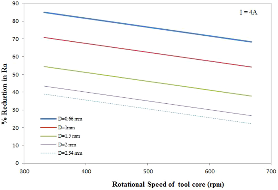
Effect of rotational speed on percentage reduction in the R_a value.

Effect of magnetizing current

The effect of magnetizing current on percentage reduction in R_a value at different working gaps and 500 r/min rotational speed of tool core is shown in Figure 7. The percentage change in surface roughness increases with an increase in the magnetizing current. The increase in magnetizing current may increase the percentage change in R_a value because the magnetic flux density in the finishing spot of MRP fluid can be increased by increasing the supply of d.c. to the electromagnet coil. Therefore, carbonyl iron particle chains keep on holding abrasives more firmly and thereby result in an increased finishing action. The continued finishing at higher magnetizing current progressively reduces the surface asperities owing to a higher bonding strength. The contour and 3D plot for the effect of the magnetizing current and rotational speed of the tool core on %ΔR_a is shown in Figure 8.

Figure 7.

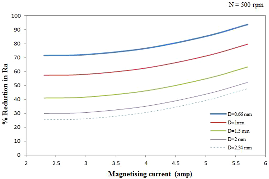
Effect of magnetizing current on percentage reduction in the R_a value.

Figure 8.

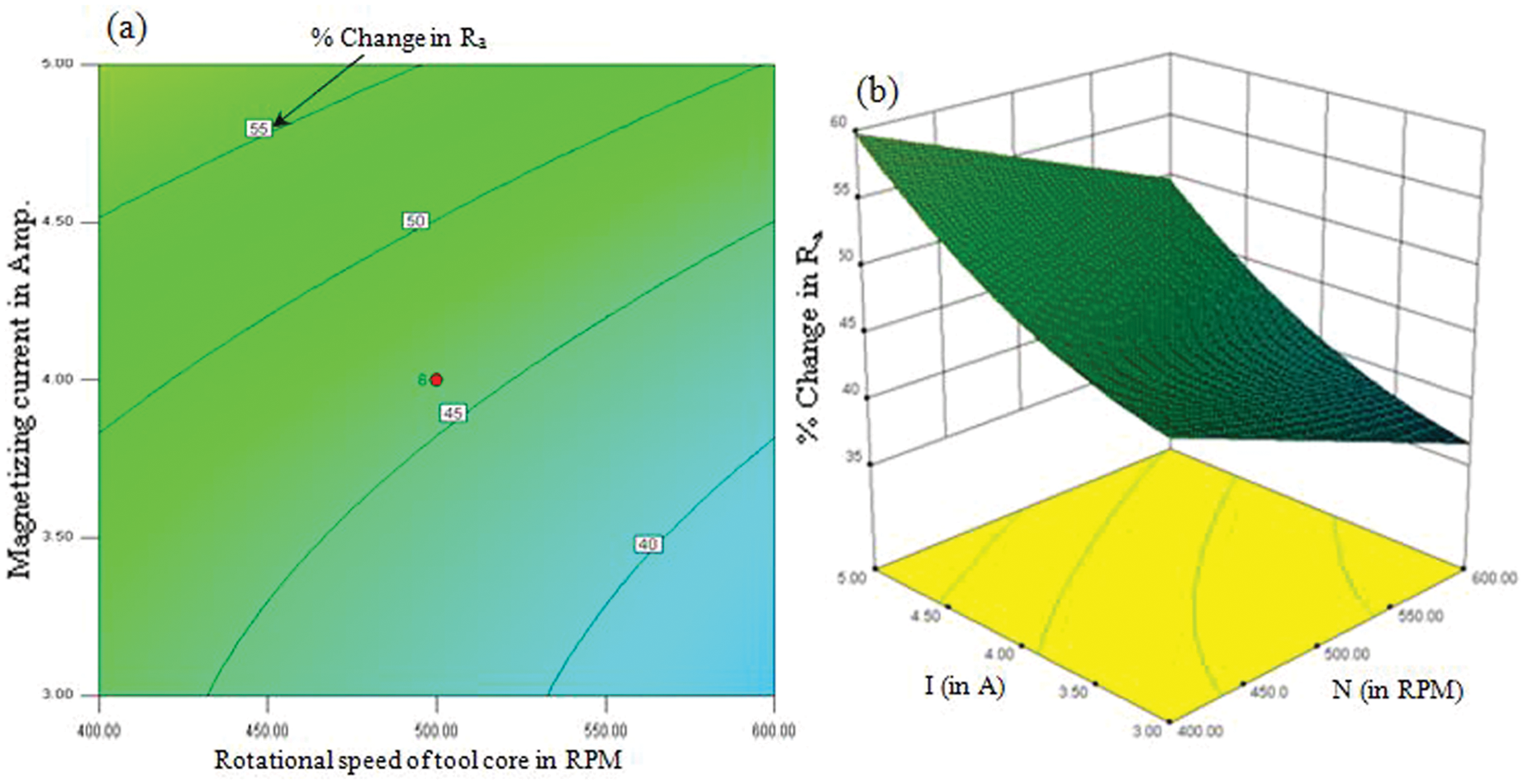
(a) Contour and (b) 3D plot of variation of the %ΔR_a value with magnetizing current and rotational speed of the tool core.

Effect of working gap

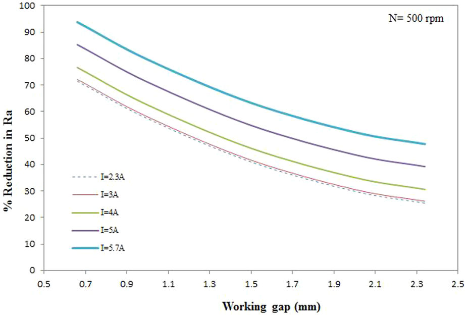
The effect of working gap on percentage reduction in the R_a value at different magnetizing currents and rotational speed of the tool core at 500 r/min is shown in Figure 9. It was observed that the percentage change in surface roughness decreases as the gap between the tip surface of the tool core and workpiece surface increases. Magnetic flux density is inversely proportional to the working gap.¹⁷ It means that when the gap between the tip surface of the tool core and workpiece surface decreases, the higher magnetic flux density can be found in the finishing spot of the MRP fluid at the tip surface of the tool core for the same supplying d.c. to the electromagnet coil, and vice versa. Therefore, at a lower working gap, the intensity of magnetization (M) increases, which further increases the interaction magnetic force (F) between two carbonyl iron particles¹⁸ as given by

Figure 9.

Effect of working gaps on percentage reduction in the R_a value.

F = \frac{μ_{0} π}{9} {(\frac{r^{2} CM}{R'})}^{2}

(6)

where r is the radius of a carbonyl iron particle, R′ is the distance between the centers of two carbonyl iron particles, and C is the collect coefficient (function of H).

Hence, as can be seen in the Figure 9, the percentage reduction in surface roughness has been increased as the working gap decreased. It can be interpreted that the magnetic field became stronger at the tip surface of the tool core for the same magnetizing current as the ferromagnetic workpiece surface got closer to the tip surface of tool core. Thus, the strong finishing spot of MRP fluid interacts with the ferromagnetic workpiece, which applies higher magnetic normal force on the workpiece surface. The corresponding shear strength of MRP fluid has been also increased, which results in an increased percentage reduction in R_a.

When the working gap increases at the same magnetizing current, the strength of the finishing spot of the MRP fluid decreases. The magnetic forces acting on the workpiece surface also decreases. Because of lower magnetic flux density was found at the tip surface of the tool core, the carbonyl iron particles are not able to hold abrasive particles strongly enough during finishing. Therefore, abrasive particles may not able to apply the necessary finishing force that is required to remove peaks from the workpiece surface. The corresponding shear strength of MRP fluid was also decreased, which results in a decrease in percentage change in R_a. The strength of the finishing spot of MRP fluid can be varied by varying either the working gap for the fixed magnetizing current or by varying the magnetizing current for the fixed working gap to get the required process performance.

The best finishing conditions are clearly captured in the experimental range of variable parameters and lies at N = 500 r/min, I = 4 A, and D = 0.66 mm. The surface finish obtained after finishing at these conditions was as low as 27.6 nm. The initial and final surface roughness profiles are shown in Figure 10(a) and (b), respectively.

Figure 10.

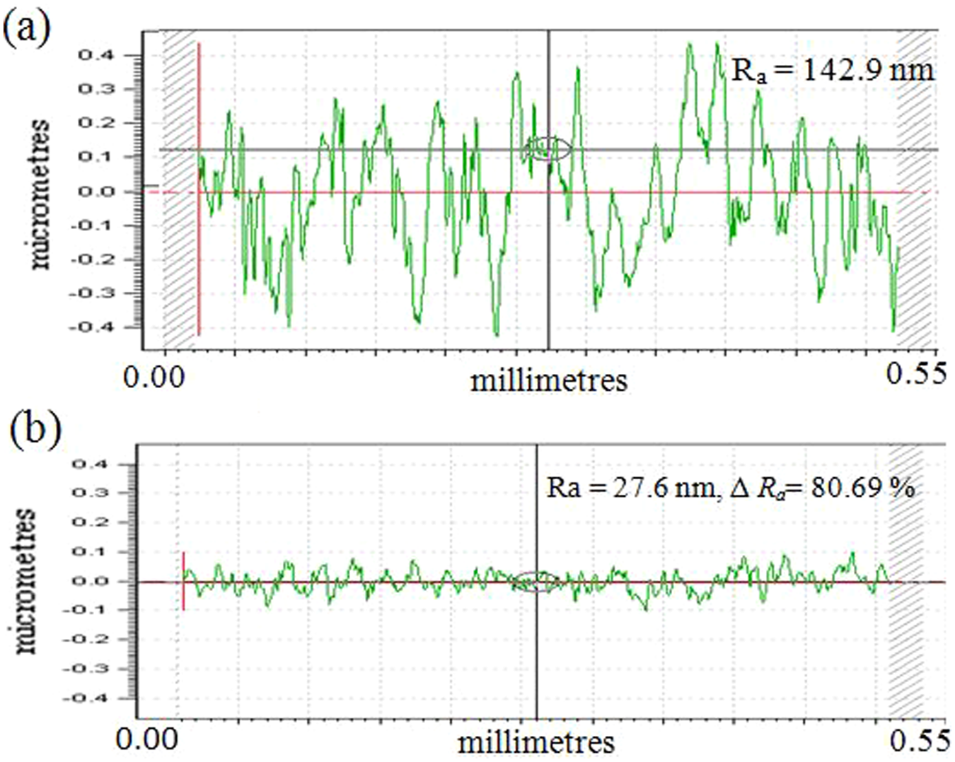
Surface roughness profile (a) before, and (b) after BEMRF for rotational speed of the tool core 500 r/min, current 4 A, and working gap 0.66 mm (Exp. No. 3 in Table 6).

The surface morphology of the workpiece was observed at these finishing conditions by using SEM at 1000× for initial and final surface of a workpiece, as shown in Figure 11(a) and (b), respectively, and it can be seen that the characteristics of the finished surface are greatly improvement compared with the initial surface of a workpiece. Few finishing abrasive marks were visible on the finished surface, which may also be removed for further finishing with comparatively fine abrasives.

Figure 11.

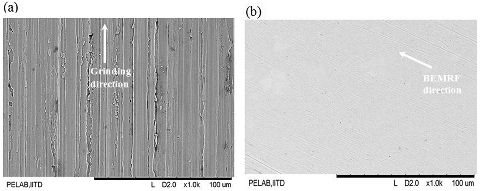
SEM micrograph at 1000× (a) before, and (b) after BEMRF for rotational speed of the tool core 500 r/min, current 4 A, and working gap 0.66 mm (Exp. No. 3 in Table 6).

Figure 12 shows the AFM images before and after finishing at the finishing conditions N = 500 r/min, I = 4 Å, and D = 0.66 mm by the BEMRF process. It can be seen that the surface quality improved significantly and the workpiece surface got flattened with some small sharp peaks and few valleys left out, which were clearly visible in the AFM images.

Figure 12.

AFM images (a) before, and (b) after BEMRF for rotational speed of the tool core 500 r/min, current 4 A, and working gap 0.66 mm (Exp. No. 3 in Table 6).

Confirmation experiments for validation of the model

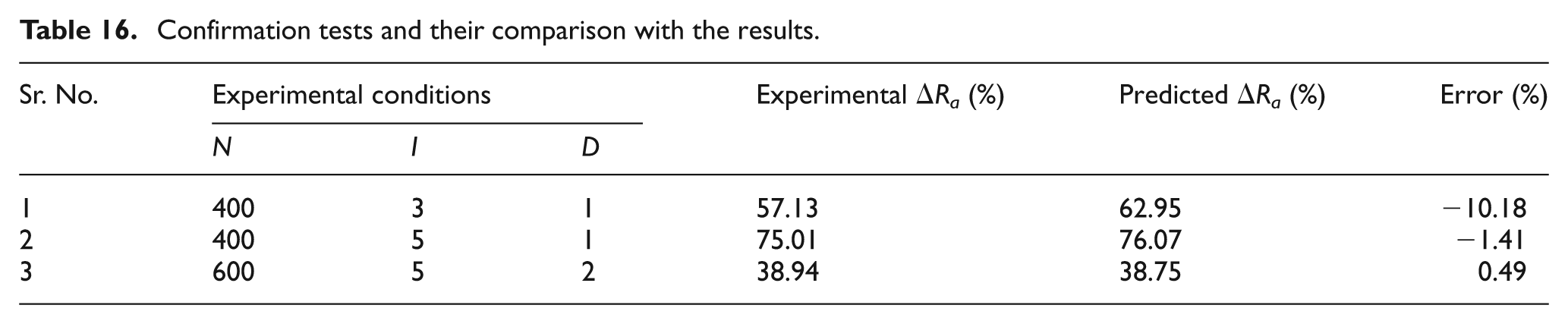
The optimum independent variable values were selected from the contour plot (Figure 8) for the confirmation tests, which lies within the ranges for which the formula was derived. Since the response surface equations of percentage change in the surface roughness were derived from a quadratic regression fit, the confirmation tests were performed to verify their validity. Three experiments have been performed to check the validity of the model given by equation (5) and the change in surface roughness was measured. The data from the confirmation tests and their comparisons, with the predicted designed-for percentage change in surface roughness, is listed in Table 16. From the analysis, it can be observed that the error between experimental and predicted values for %ΔR_a lies within −10.18% to 0.49%. This confirms good reproducibility of the experimental results.

Table 16.

Confirmation tests and their comparison with the results.

Sr. No.	Experimental conditions			Experimental ΔR_a (%)	Predicted ΔR_a (%)	Error (%)
	N	I	D
1	400	3	1	57.13	62.95	−10.18
2	400	5	1	75.01	76.07	−1.41
3	600	5	2	38.94	38.75	0.49

Conclusion

An experimental study through statistical design was conducted for nanofinishing of ferromagnetic workpieces using a newly developed BEMRF process. The working gap is found to be the most significant factor in affecting percentage change in the surface roughness (R_a) value of the ferromagnetic workpiece. Analysis of design of the experiment results reveals no significant interaction between the process parameters that were studied, such as rotational speed of the tool core, magnetizing current, and working gap. The best surface finish R_a value obtained on a ferromagnetic workpiece was 27.6 nm from initial R_a value 142.9 nm at the finishing conditions of N = 500 r/min, I = 4 Å, and D = 0.66 mm. This finishing conditions lie within the experimental range of variables for MRP fluid used with 20% volume carbonyl iron particles, 20% volume SiC abrasives of mesh number 800, and 60% volume base fluid of paraffin oil plus AP3 grease medium.

Footnotes

References

This research received no specific grant from any funding agency in the public, commercial, or not-for-profit sectors.

References

Mulik

Pandey

. Magnetic abrasive finishing of hardened AISI 52100 steel. Jain VK. Advanced machining processes. Allied Publisher Pvt. Ltd., New Delhi, 2004.

Kordonski

Jacobs

. Magnetorheological finishing. Int J Mod Phys B 1996; 10: 2857–2865.

Shorey

Jacobs

Kordonski

. Experiments and observations regarding mechanisms of glass removal in magnetorheological finishing. Appl Optics 2001; 40(1): 20–33.

Shorey

. Mechanisms of material removal in magnetorheological finishing (MRF) of glass. PhD Thesis. University of Rochester, NewYork, 2000.

Bulsara

Ahn

Chandrasekar

. Mechanics of polishing. Trans ASME J Appl Mech 1998; 65: 410–416.

Kordonski

Golini

Dumas

. Magnetorheological suspension-based finishing technology. Proc SPIE 1998; 3326: 527–535.

Golini

Kordonski

Dumas

. Magnetorheological finishing (MRF) in commercial precision optics manufacturing. Proc SPIE 1999; 3782: 80–91.

Kim

Lee

Min

. Surface finishing and evaluation of three-dimensional silicon microchannel using magnetorheological fluid. J Mfg Sci Eng 2004; 126: 772–778.

Seok

Kim

Kyung

. A study on the fabrication of curved surfaces using magnetorheological fluid finishing. Int J Mach Tools Mf 2007; 47: 2077–2090.

10.

Cheng

Yam

Wang

. Experimentation on MR fluid using a 2-axis wheel tool. J Mater Process Technol 2009; 209(12–13): 5254–5261.

11.

Jacobs

. Manipulating mechanics and chemistry in precision optics finishing. Sci Technol Advd Mater 2007; 8: 153–157.

12.

Miao

Lambropoulos

Jacobs

. Process parameter effects on material removal in magnetorheological finishing of borosilicate glass. Appl Optics 2010; 49(10): 1951–1963.

13.

Singh

Jha

Pandey

P M

. Design and development of nanofinishing process for 3D surfaces using ball end MR finishing tool. Int J Mach Tools Mf 2011; 51: 142–151.

14.

Kordonski

Shorey

. Magnetorheological (MR) jet finishing technology. J Intell Mater Syst Struct 2007; 18: 1127–1130.

15.

Montgomery

D C

. Design and analysis of experiments. 5th ed. New York: John Wiley & Sons Inc, 2001.

16.

Jha

Jain

. Parametric analysis of magnetorheological abrasive flow finishing process. Int J Mfg Technol Mgmt 2008; 13: 308–323.

17.

Sidpara

Jain

. Experimental investigations into forces during magnetorheological fluid based finishing process. Int J Mach Tools Mf 2011; 51: 358–362.

18.

Huang

Zhang

Liu

. Effect of magnetic field on properties of MR fluid. Int J Mod Phys 2005; B19: 597–601.

Parametric analysis of an improved ball end magnetorheological finishing process

Abstract

Keywords

Introduction

BEMRF process variables

Rotational speed of tool core (N)

Magnetizing current (I)

Working gap (D)

Design of experiments

Response surface regression analysis

Results and discussion

Effect of rotational speed of tool core

Effect of magnetizing current

Effect of working gap

Confirmation experiments for validation of the model

Conclusion

Footnotes

References

References