
Abstract
This article deals with a new approach to understand the magnetic-field-assisted nano-finishing process in which computational fluid dynamics is used to simulate the forces. A finite element method is used to evaluate the magnetic field intensity, mathematical modelling is applied to model the nano-finishing operation, and the experiments are conducted to compare the experimental results with the simulated results. A flexible polishing tool comprising a magnetorheological polishing medium is used for this process. The relative motion between the polishing medium and the workpiece surface provides the required finishing action. In the present work, a two-dimensional computational fluid dynamics simulation of a magnetorheological polishing medium inside the workpiece fixture is performed to evaluate the axial and radial stresses developed owing to the flow of magnetically stiffened magnetorheological polishing medium. A finite element analysis is performed in order to find out the direction and the magnitude of the magnetic field. A microstructure of the mixture of magnetic and abrasive particles in the magnetorheological polishing medium is proposed in order to calculate forces acting on an active abrasive particle. Modelling of the surface finish is performed after analysing the surface roughness profile data. Further finishing experiments are conducted in order to compare the simulated surface roughness value with the experimental results and they are found to agree well.
Keywords
Introduction
In the magnetic-field-assisted finishing (MFAF) process, a magnetorheological polishing (MRP) medium reciprocates inside the workpiece/fixture assembly with the help of a hydraulic unit. In the finishing zone that is under the magnetic field, carbonyl iron particles (CIPs) in the MRP medium get magnetized and form chain-like structures. Figure 1 shows the schematic diagram of the MFAF experimental set-up (Figure 1(a)) and finishing mechanism (Figure 1(b)) of the MFAF process. As shown in Figure 1(b), before entry and after exit from the workpiece fixture, the polishing medium behaves as a Newtonian fluid because there is no effect of a magnetic field in these zones. Once the medium enters the finishing zone under a magnetic field, the polishing medium becomes stiff and starts behaving as a Bingham plastic fluid.
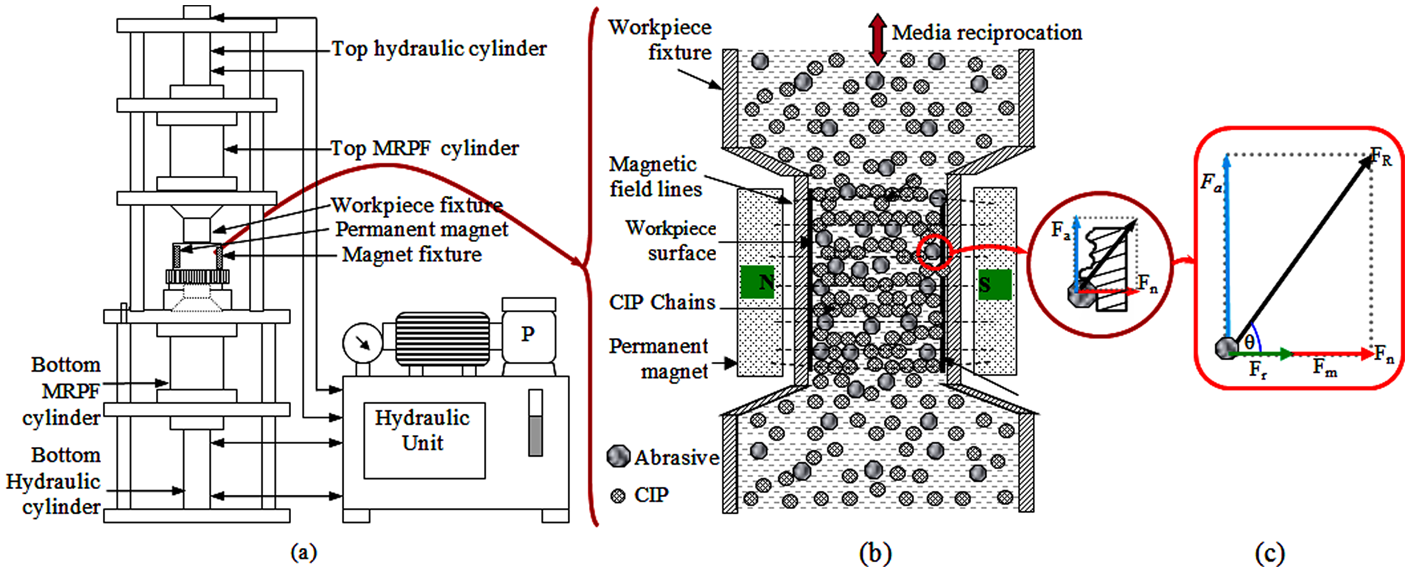
(a) Schematic diagram of MFAF experimental set-up, (b) mechanism of finishing, (c) chip formation and force components acting on an abrasive particle in the finishing zone.
The experimental set-up consists of two permanent magnets (made of Nd–Fe–B alloy), which are attached to the magnet fixture and are placed in such a way that the magnet poles are opposite to each other. Two different grades of permanent magnets (N17 and N48, Table 1) are used during finishing. Inside the magnet fixture, there is a cylindrical workpiece fixture (made of brass) having internal slots in which flat stainless steel workpieces (35 × 5 × 2.5 mm) are mounted just in front of the magnets for finishing (Figure 1(b)).
Properties of the Nd–Fe–B permanent magnet with dimension.
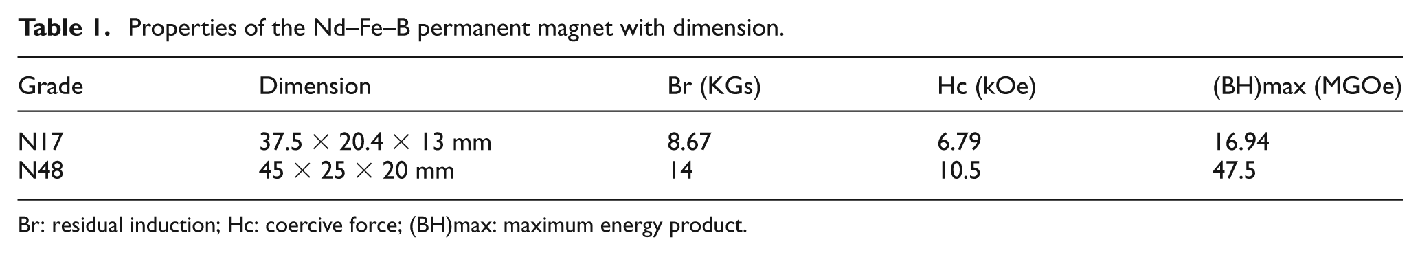
Br: residual induction; Hc: coercive force; (BH)max: maximum energy product.
Figure 1(c) shows the formation of the chip and forces acting on an abrasive particle in the MFAF process. Abrasive particles held by the CIPs are pressed against the surface of the workpiece owing to the magnetic force, Fm. In the MFAF process, the axial/cutting force (i.e. shear force) (Fa), owing to the reciprocation of the medium by the hydraulic unit, acts parallel to the axis of the fixture and cuts the roughness peaks (Figure 1). This extrusion pressure also generates radial force, Fr, which helps the abrasive particles in indenting into the workpiece surface. The total normal indentation force (

In the present work, a two-dimensional (2D) computational fluid dynamics (CFD) simulation of the flow of the MRP medium has been carried out to evaluate the axial and radial stresses developed during finishing. A finite element (FE) analysis of the MRP medium in the finishing zone has been carried out to simulate direction and magnitude of the magnetic field. The structure of the CIPs chains has been proposed to calculate forces acting on the abrasive particles. A surface roughness simulation model based on the surface roughness profile data has been developed and the predicted roughness values are compared with the experimental results. The MRP medium used during polishing for all the cases discussed in this article consists of CIPs of CL grade (diameter = 25 μm) purchased from BASF Germany, SiC abrasive particles with 600 mesh size (diameter = 25.33 μm), 12 vol.% grease, and 48 vol.% paraffin oil.
CFD simulation of MRP fluid flow
The aim of this section is to numerically calculate the axial and radial velocity in the computational domain from which axial and radial stresses along the workpiece fixture wall are calculated.
Governing equations and viscosity model
The mathematical representation of the flow of the MRP medium in the MFAF process involves basic equations of continuity (equation (2)) and momentum (equation (3)) 1 in combination with a suitable rheological constitutive equation. Tensor notations have been used

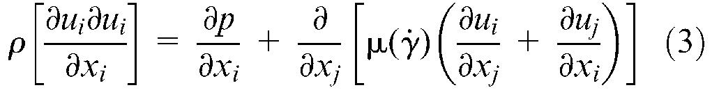
where, ρ is density of the fluid, p is pressure, and

where

In the present simulation the effect of heat generation owing to viscous dissipation has not been considered. However, for more accurate modelling the continuity, momentum and energy equations should be solved simultaneously as the temperature rise will also affect the viscosity of the fluid (viscosity will decrease exponentially with temperature).
Furthermore, in this study a quasi-steady state has been assumed. The fluid is incompressible. The flow is modelled in a time-averaged sense. Thus, the unsteady terms (owing to reciprocating motion) in the r- and z-momentum equations disappear.
In the current analysis, a Bingham plastic non-Newtonian constitutive viscosity model that is viscoplastic in nature
2
has been employed for handling the viscous force term in equation (3). The Bingham plastic model describes materials with yield stress,


where,

Equation (6a) mimics the ideal Bingham plastic model for
The
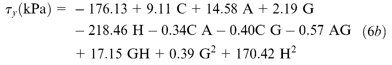
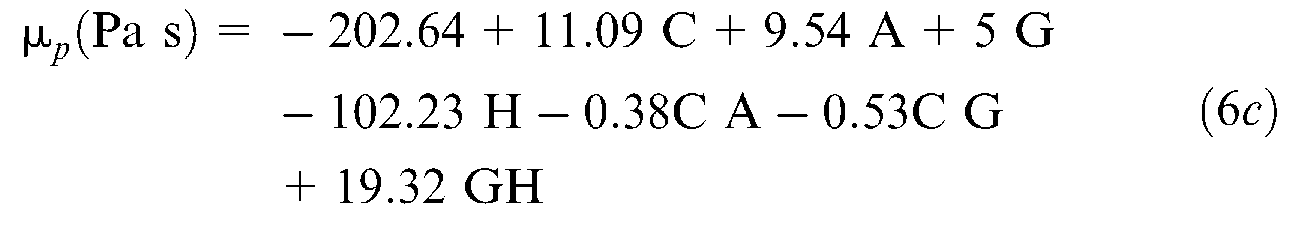
Here, C, A, G are volume concentrations of the CIPs, abrasive particles, and grease, respectively. H is the applied magnetic field.
Boundary conditions
The schematic diagram of the computational domain for one-half of the workpiece fixture is shown in Figure 2. The computational domain is divided into two zones (i.e. Zone I and Zone II). The MRP fluid behaves as a Newtonian fluid in Zone I since the magnetic field is not applied in this zone. In the finishing zone (Zone II), owing to the application of the magnetic field, MRP fluid behaves as a Bingham plastic fluid. In the latter part of Zone I there is a gentle contraction (a taper angle of 45° is provided). This is done in order to extrude the polishing medium from one medium cylinder (internal diameter = 80 mm) into the workpiece fixture (internal diameter = 24 mm and external diameter = 30 mm) in the finishing zone (Zone II), and after that in same way to the receiving medium cylinder on the other side.
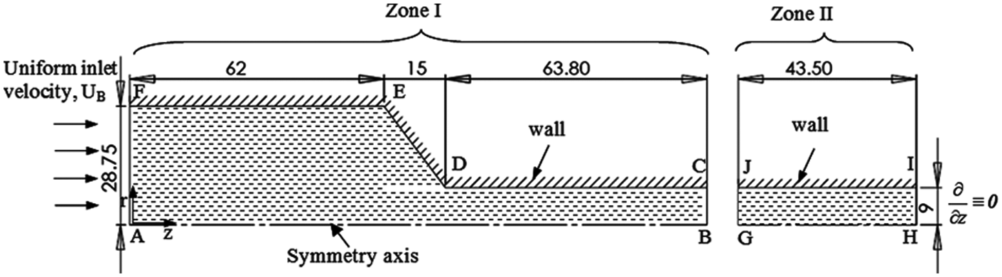
Schematic diagram of the computational domain (half of the physical domain) and the boundary conditions(all dimensions are in mm).
The boundary conditions applied in Zone I are as follows: at inlet (i.e. z = 0) uniform velocity profile (UB) and at outlet, a fully developed flow condition are considered. Along the wall, a no-slip boundary condition is applied. Along the axis of the cylindrical fixture, an axi-symmetric boundary condition is applied.
Similarly, the boundary conditions for Zone II are as follows: the axial and radial components of the outlet velocity profile obtained from Zone I are taken as the components of the inlet velocity profile for Zone II. Zero axial gradients ((∂/∂z)≡0)) for all flow variables are imposed at the outlet. The exit boundary condition in Zone II is justified by the fact that the flow is fully developed at the outlet as the hydrodynamic entry length is very small because of a very low Reynolds number of the flow arising out of a very high fluid viscosity. A no-slip boundary condition is applied at the wall and an axi-symmetric boundary condition is applied along the axis of the cylindrical fixture.
Numerical method
The following assumptions are made to simplify the analysis.
The medium is homogeneous.
The flow is quasi-steady, incompressible and laminar.
The flow is axi-symmetric (i.e. at
There is no swirling motion of the fluid (i.e.
A well established commercial CFD package ‘FLUENT’ (Version 6.3.26) is utilized to solve the continuity (equation (2)) and momentum (equation (3)) equations of fluid flow along with the constitutive viscosity model (equation (6a)). A second-order upwind scheme is used to discretize both convective and diffusive terms. A SIMPLE (semi-implicit method for pressure-linked equations) algorithm is used for the coupling of pressure and velocity.
5
Double precision with 10 decimal points is used for the simulation to reduce round-off errors. The iterations are stopped whenever the scaled residuals for the solutions for the two components of velocity (
Grid independence test
A grid independence test of the computation has been conducted for both Zones I and II. The maximum value of outlet axial velocity profile (umax) for both zones have been calculated and are provided in Table 2. The maximum value of per cent change in umax

of 1% is chosen as a criterion for testing grid independence for different grid resolutions. Three different grids (coarse, base, and refined mesh) consisting of quadrilateral cells are considered for both zones (Table 2).
Results of grid independence test for different grid-resolutions in Zones I and II.
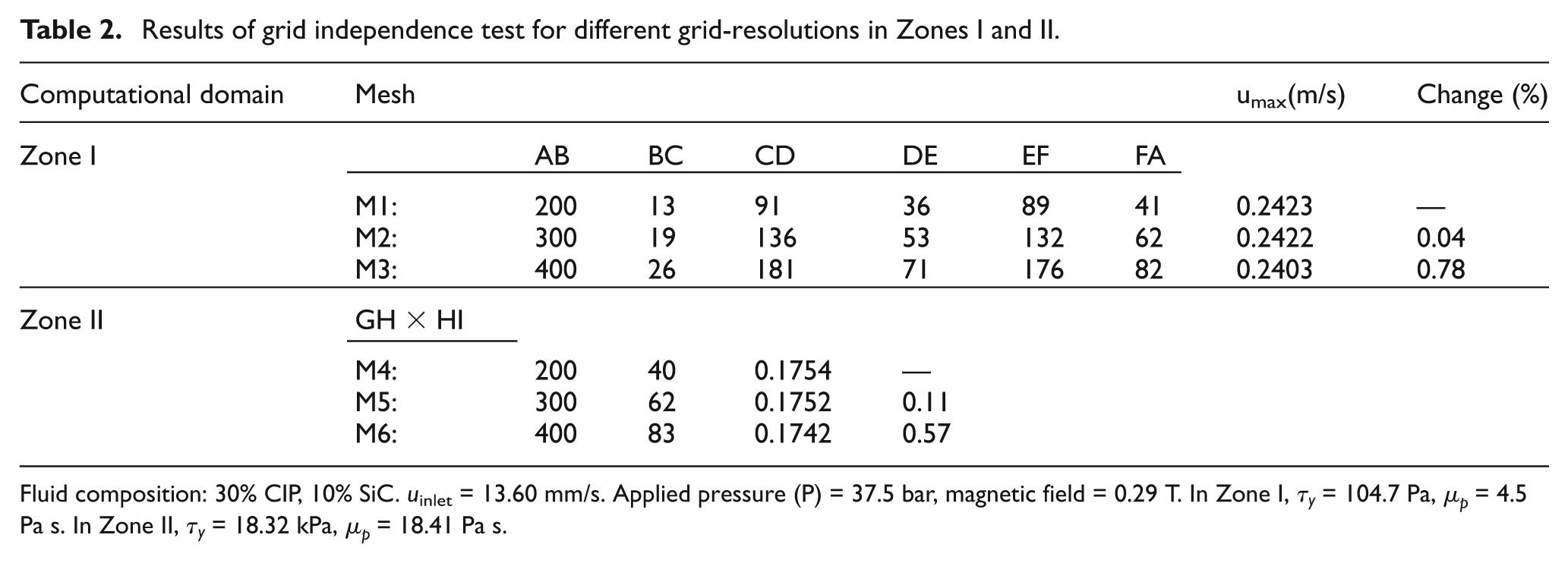
Fluid composition: 30% CIP, 10% SiC. uinlet = 13.60 mm/s. Applied pressure (P) = 37.5 bar, magnetic field = 0.29 T. In Zone I,
The off-state rheological properties of the MRP medium (required for the simulation of the MRP medium in Zone I) are measured using a Anton-Paar parallel plate rheometer. Although MR fluid behaves as a Newtonian fluid without application of a magnetic field, a very small amount of yield stress is observed in the shear stress plot. It is because the aforesaid polishing medium consists of 42% solid particles (32% CIP, 10% SiC) that are micron sized and the MRP fluid is very thick, even without the application of a magnetic field. Therefore, the shear stress values are fitted with the Bingham plastic model and the corresponding rheological properties (
From Table 2, it can be found that there is not much difference between outlet velocities (for both Zones I and II) for three different grid resolutions. Also, percentage change in umax in Table 2 is within 1% of one grid level to the more refined one. Hence, the lowest number of grid points in the range, that is M1 grid (for Zone I) and M4 grid (for Zone II), has been selected for saving central processing unit (CPU) time and utilized for further computations.
Validation with the analytical solution
The radial variation (r) of outlet axial velocity (u) profiles of simulation results is compared with the analytical solution of the fully developed Bingham plastic pipe flow (equations (7) and (8)),
6
and it is shown in Figure 3 for Re = 0.001 at various Bingham numbers. The axial velocity (
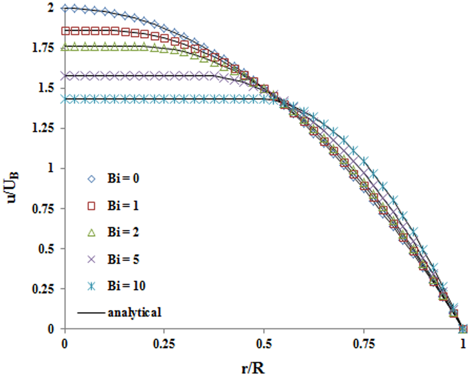
Comparison of outlet axial velocity profiles between simulation results and analytical solution of the fully developed Bingham plastic pipe flow for different Bingham numbers(Re = 0.001).
and the axial velocity (
where,

For Newtonian fluid, Bn = 0 and at the other extreme of an unyielded solid, Bn→∞, 2 the Reynolds number based on the momentum correction coefficient method for Bingham plastic fluid is given as

The apparent viscosity (
Velocity distribution of the polishing medium
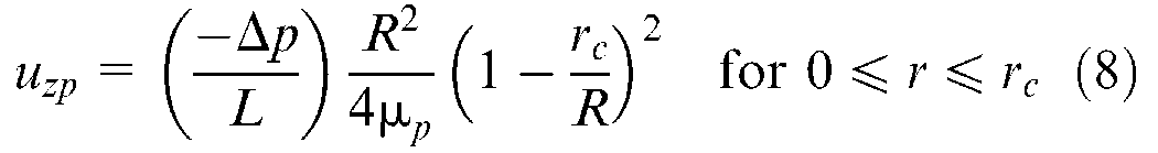
Figure 4(a) shows the axial velocity contour plot in Zone I. From Figure 4(a), it is observed that there is a plug flow region near the exit of Zone I, although the magnetic field is not applied in this zone. The reason for this has already explained above (‘Grid independence test’) owing to the off-state yield stress property of the MRP fluid used. The pattern of velocity distribution in Zone II is shown in Figure 4(b). The axial velocity contour plot (Figure 4(b)) indicates that there is a solid core region near the axis of the cylindrical fixture where the medium flows with maximum velocity and the velocity decreases non-linearly, radially outwards from the centre to the fixture wall, where it becomes zero. This confirms the medium flow distribution of the viscoplastic (Bingham plastic) fluid. 6 Also, from Figure 4(b) it can be observed that there is development of the boundary layer near the inlet section up to approximately 0.01 m, after which the flow becomes fully developed.
Axial velocity distribution (contour plot) of the flow of polishing medium in (a) Zone I (
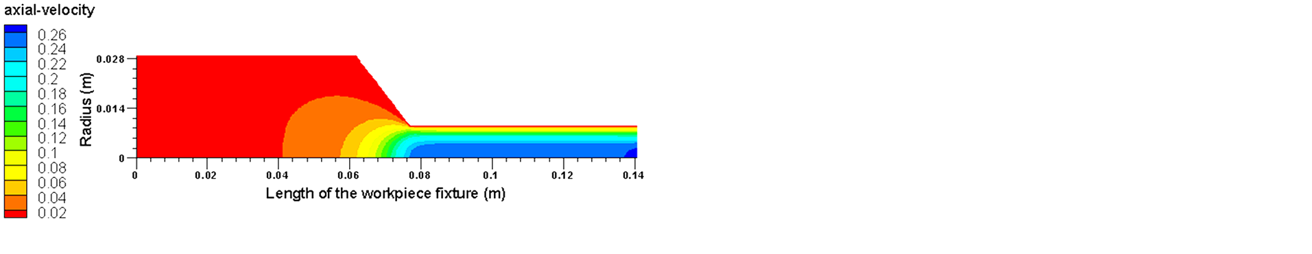
Figure 5(a) shows the velocity distribution (vector plot) for the flow of polishing medium in the half physical domain in the finishing zone (Zone II). From this figure it can be observed that the velocity vectors are slightly inclined towards the wall near the inlet section (before the fluid gets fully developed) because of the application of the magnetic field just outside the workpiece fixture. It helps the abrasive particles in the polishing medium to efficiently scoop up the surface asperities from the workpiece surface. This phenomenon of velocity distribution is not visible in the MFAF process in Zone II without the application of the magnetic field as shown in Figure 5(b). This phenomenon leads to the non-finishing of the workpiece surface for the MFAF at zero magnetic field. 8
Velocity vector plot of the flow of polishing medium in Zone II for half of the physical domain at (a) 0.5 T magnetic field (
The yielded and unyielded regions of the MRP medium are clearly visible in Figure 5(a) where the unyielded region is almost extended towards the fixture wall maintaining a very small yielded region near the wall. In the unyielded region, as the fluid is not sheared, the CIPs chain structure remains intact and can provide a higher bonding force to the abrasive particles than the yielded region (where the CIPs chain structures are sheared). Hence, the higher unyielded region and lower yielded region of the flow of the MRP medium as in the current case gives rise to a higher finishing efficiency in the MFAF process.
The flow becomes fully developed (visible in the simulated axial velocity contour plot in Zone I, Figure 4(a)) near 0.1 m length along the length of the workpiece. After the flow becomes fully developed there is no change in the velocity profile. Similarly, the fully developed flow condition is achieved near 0.01 m in Zone II as shown in Figure 4(b) and Figure 5(a).
Magnetic field simulation of the MRP fluid
A commercial finite element method (FEM) package of Maxwell equation solver Ansoft Maxwell® is used to simulate the magnetic field (B) of the MRP medium in the finishing zone in between two opposite permanent magnets as in the original finishing condition (Figure 6(a)). The simulated magnetic field (B) is utilized to calculate the magnetic force (Fm) applied on an abrasive particle through surrounding CIP chains. It is necessary to mention that the MRP medium considered here is in a static state although the medium gets sheared during polishing. At first, the simulated magnetic field (B) without the MRP medium is compared with the experimentally measured magnetic field using a Gaussmeter (with 1 Gauss (= 10–4 T) accuracy) in between two permanent magnets of the MFAF set-up. These comparison results are shown in Figure 7 for both N17 and N48 grade permanent magnets. From Figure 7, it can be observed that these two results are almost matching. Hence, the magnetic field (B) is simulated using the Ansoft Maxwell solver in the MRP medium in the finishing zone, and the same is used for magnetic force calculation during surface roughness evaluation.
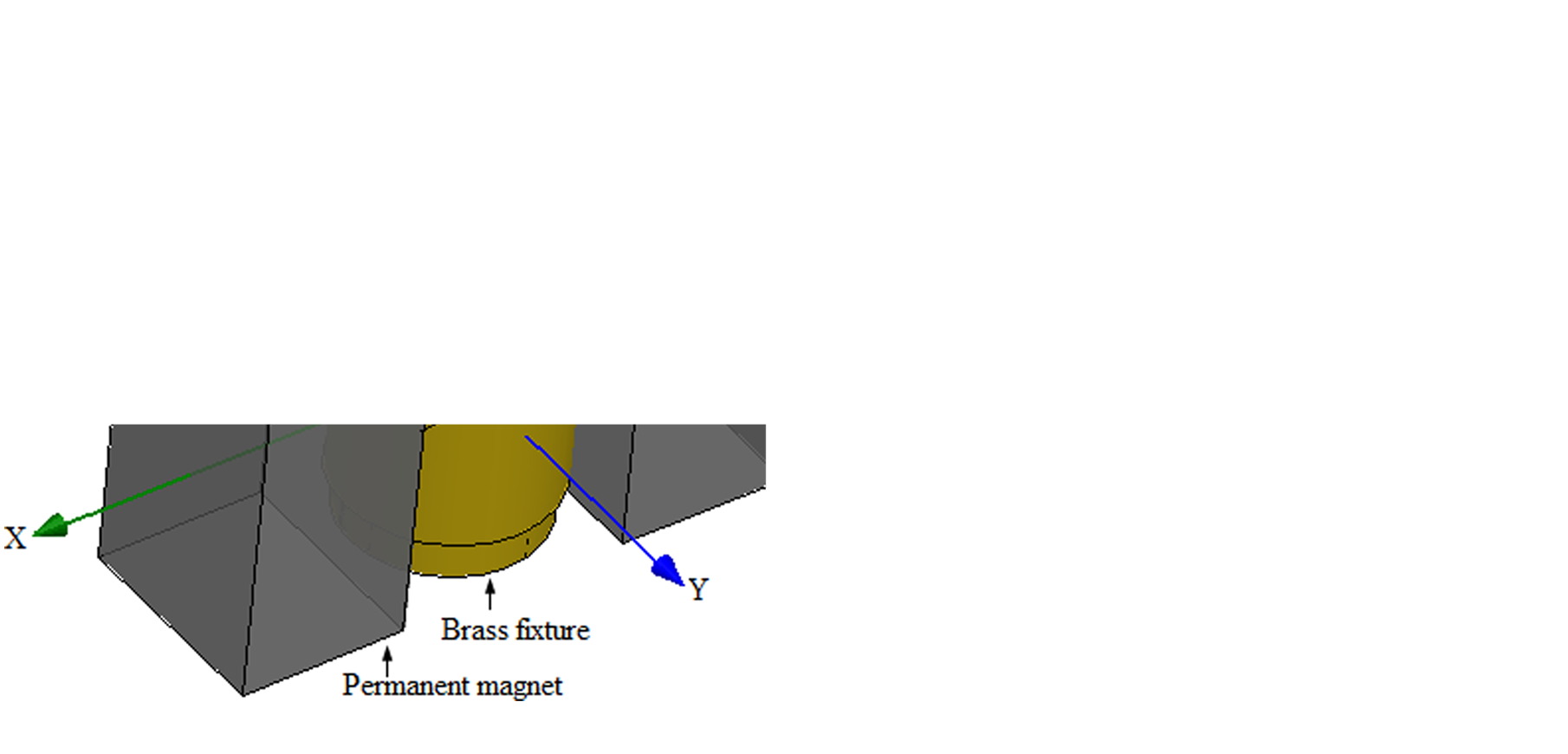
(a) Schematic diagram of the workpiece fixture with permanent magnets in the finishing zone, (b) simulated magnetic field vector in the finishing zone using an N48 magnet.
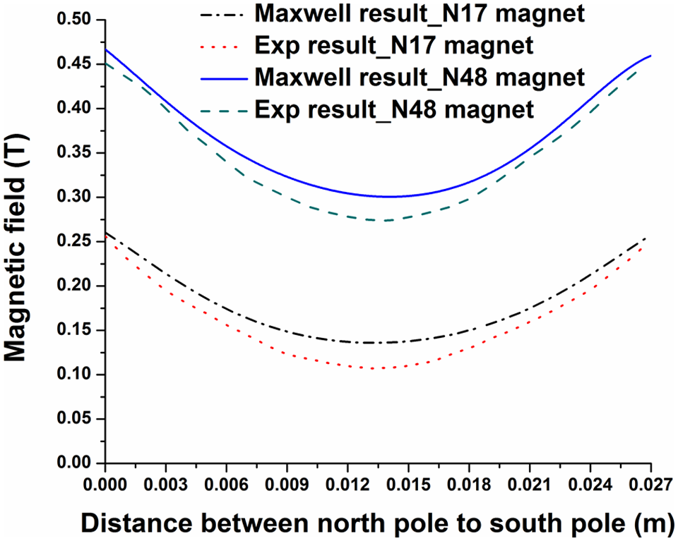
Comparison between simulated and experimentally measured magnetic field, B (Tesla), in between two opposite permanent magnets.
Figure 6(b) shows the simulated magnetic field vector plot in the finishing zone. From Figure 6(b), it is observed that the magnetic field vector lines are almost perpendicular to the workpiece surface (i.e. parallel to the X-axis) inside the polishing medium. Hence, a normal component of the magnetic force, Fm (equation (1)) is considered for the simulation of forces in this work. However, away from the centre of the workpiece fixture (i.e. near the fixture wall in both +Y and –Y directions) magnetic lines of force become slightly inclined with the X-axis.
The force on a small ferromagnetic particle of mass ‘m’ in the magnetic field at a distance (x) is given as 9

where,

where, the magnetization of the MRP medium is different magnetic fields (B) measured from a parallel field vibrating sample magnetometer (VSM) (model EV5, ADE Magnetics, USA) at room temperature.
CIPs chain structure and active abrasive particles
Tao 10 theoretically found that the CIPs chains in MR fluid form a crystalline structure, i.e. a body-centred tetragonal (BCT) structure. In the present case, for the ease of calculation of the indentation force on the workpiece surface, it is assumed that the CIPs chain structure just adjacent to the workpiece surface form a half-body-centred cubic (BCC) structure (as the MRP fluid consists of almost the same size CIP and SiC particles) and the active abrasive particle is touching the workpiece surface. In this chain structure it is assumed that one abrasive particle is surrounded by eight CIPs (Figure 8(a)). This chain structure is repeated radially forming a long chain in the magnetic field direction (Figure 8(b)) in between two workpieces inside the workpiece fixture in front of two opposite permanent magnets.
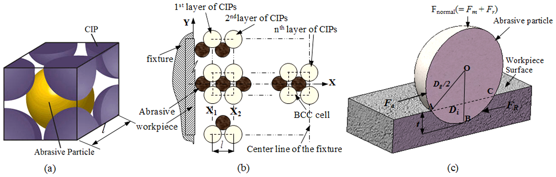
(a) The assumed unit BCC microstructure of abrasive and CIPs, (b) magnified view of the CIPs chain structure inside half the physical domain of the workpiece and its fixture in the finishing zone, and (c) cross-sectional view of an abrasive particle penetrating into the workpiece surface and the forces acting on it.
As shown in Figure 8(b), an active abrasive particle touching the workpiece surface is surrounded by four magnetic particles. Therefore, the magnetic force transmitted to an active abrasive particle is found to be Fm after balancing the forces in the magnetic field direction. It is assumed that the magnetic force is transferred to the active abrasive particle touching workpiece surface through all layers of the CIPs chains. The magnitude of magnetic force changes from its maximum value at the inner wall of the cylindrical fixture to a minimum value at the centre owing to the variation of magnetic field as shown in Figure 7. Hence, the total magnetic force (

where,

where

Here,
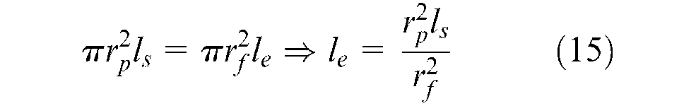
where

where l is the length of the BCC cell or linear spacing between the centre of two adjacent active abrasive particles in CIP chains (Figure 8(b))

Modelling of material removal
The following assumptions are adopted for the analysis of material removal during the MFAF process: All abrasive particles are approximated to be spherical in shape 11 of the same size, and average diameter of the abrasive particle (dg) is calculated from the mesh size number (Me) as dg = (15,200/Me) (μm). Each abrasive particle consists of a single active cutting edge. The load on each abrasive particle is assumed to be constant, hence each one of them creates the same penetration depth on the workpiece surface.
After calculating the normal indentation force (Fn) from equation (1), the indentation diameter (
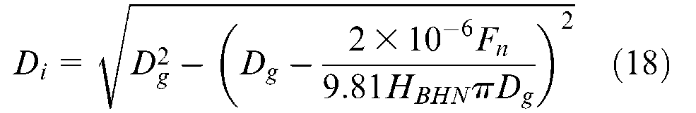
where

During shearing of a roughness peak by an active abrasive particle on the work surface, the axial shear force (


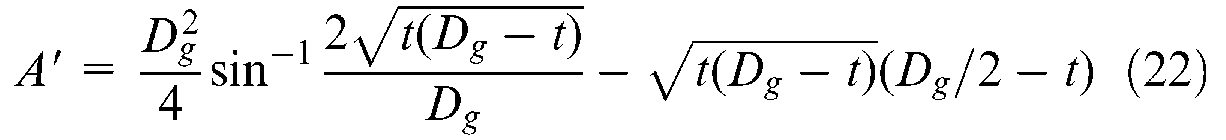
where A is cross-sectional area of the spherical abrasive particle,
From CFD simulation, the axial stress at the fixture wall at the lowest extrusion pressure of 32.5 bar and N48 magnet is calculated as 39.96 kPa with a MR fluid composition of 26.67% CIP, 13.33% SiC. Substituting these values into equations (20)–(22),
Modelling of surface finish
Modelling of surface finish is performed after analysing the surface roughness profile data obtained from the surface roughness measuring instrument. In the section ‘Modelling of material removal’, it is calculated that the axial force on an abrasive particle is 107 times higher than the resistance force by the strength of the material. Also, from CFD simulation it has been found that the axial stress is a third-order magnitude higher than that of the radial stress. From the data points of the surface roughness profile it is found that the width of the valley along the mean line is 1.25 μm and the diameter of the abrasive particle is 25.33 μm which is much higher than the width of the valley. Hence, it is difficult for an active abrasive particle to enter inside the valley for material removal during finishing. Considering these two facts, it is assumed that, while cutting the roughness peak during the MFAF process, an active abrasive particle will be translated horizontally in a straight line in the direction of the fluid flow. The steps consisting of the surface roughness simulation model is discussed in the following paragraph. The surface roughness calculation from profile data points is explained schematically in Figure 9 for a few peaks and valleys of the roughness profile. The flow chart of the algorithm to calculate surface roughness is shown in Figure 10.
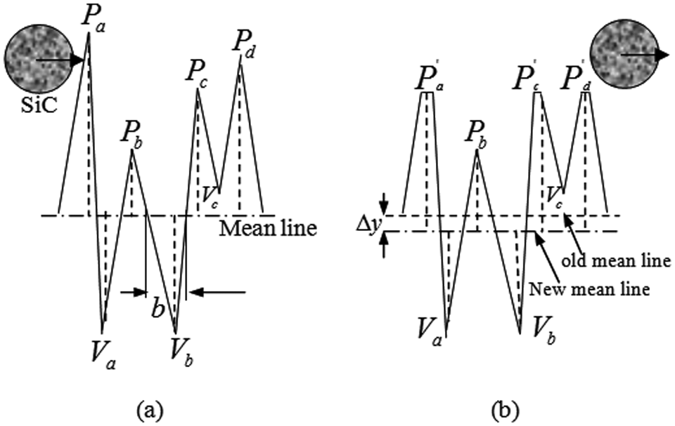
(a) Abrasive particle approaching initial peaks/valleys; (b) new peak heights updated after one indentation depth (t).Δy is the shifting of the position of the mean line after each stroke.
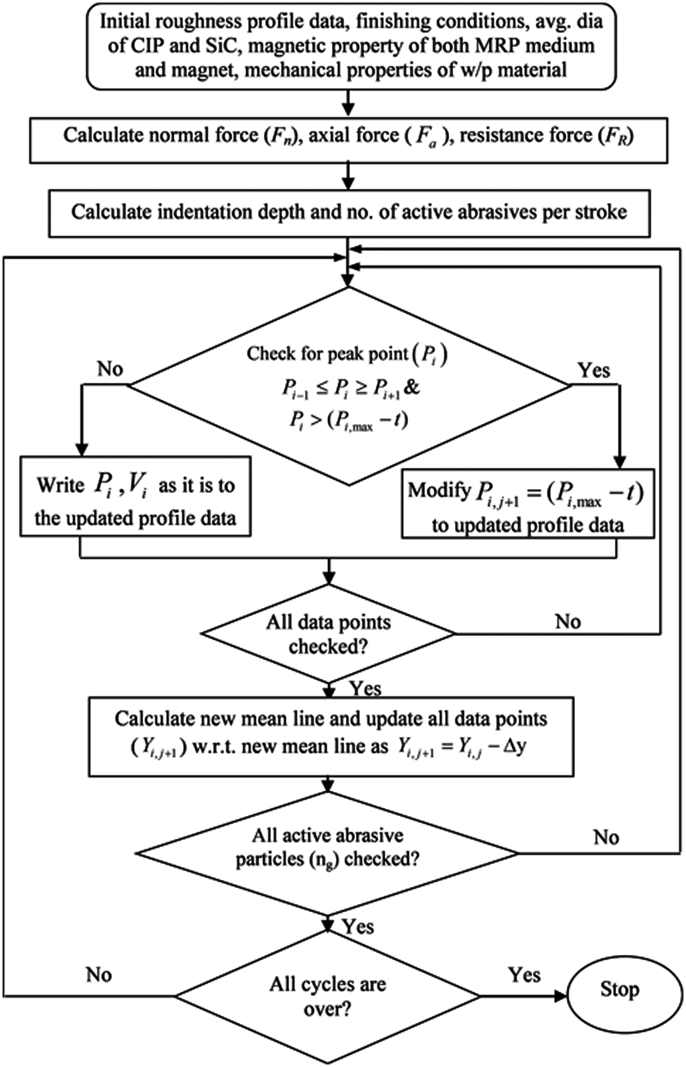
Flow chart for the simulation of surface roughness profile in the MFAF process.
Step 1. The initial surface roughness profile data points from the surface roughness measuring instrument are stored in an array. After that the peak points of the profile data are identified if the condition of
Step 2. It is important to note that only those points that are identified as the peak points (
Step 3. Therefore, in the next cycle (j+1) the new height of the ith roughness peak (

where
From Figure 9, it can be seen that the new peak heights updated after cutting one abrasive particle is given as
Step 4. After each iteration all the data points that were separated earlier into two arrays consisting of peak points (
Step 5. One more thing to notice is that the roughness value is calculated with respect to the mean line of the profile, which can be defined as the line that divides the profile in such a way that the area above and below the mean line are equal. After each iteration, some material from the upper half of the mean line is removed, and thus, there would be a shift in the position of the mean line (Δy). Therefore, after each iteration, the new mean line of the roughness profile is calculated and accordingly all the data points (

Step 6. The centreline average surface roughness value (Ra), calculated from the profile data points (

where, n is the number of data points.
Results and discussion
In this section, the simulation results of fluid flow analysis, magnetic field analysis, and final surface roughness profiles at different CIP concentration, finishing cycles, and extrusion pressures are discussed. The experimental data of the initial surface roughness profile, obtained from the surface roughness measuring instrument (‘Federal Surfanalyzer 5000’ with an accuracy of 1 nm), are utilized for the simulation of the final surface roughness profile after finishing of the stainless steel workpiece and is validated with the experimental results. The finishing conditions during experimentation and simulation are kept the same.
Effect of CIP concentration
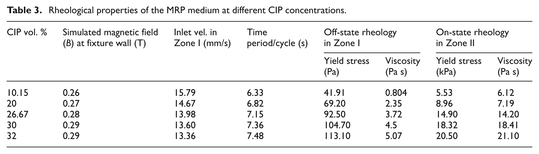
The finishing experiments are conducted with the MRP medium of different CIP concentrations (Table 3) keeping other constituents of the fluid fixed. Owing to an increase in the CIP concentration in the MRP medium, the induced magnetic field (B) inside the workpiece fixture is also increased. The simulated magnetic field on the workpiece surface, rheological properties of the MRP fluid, measured inlet velocity, and the time period for the single finishing cycle in Zone I are provided in Table 3 for different CIP concentrations.
Rheological properties of the MRP medium at different CIP concentrations.
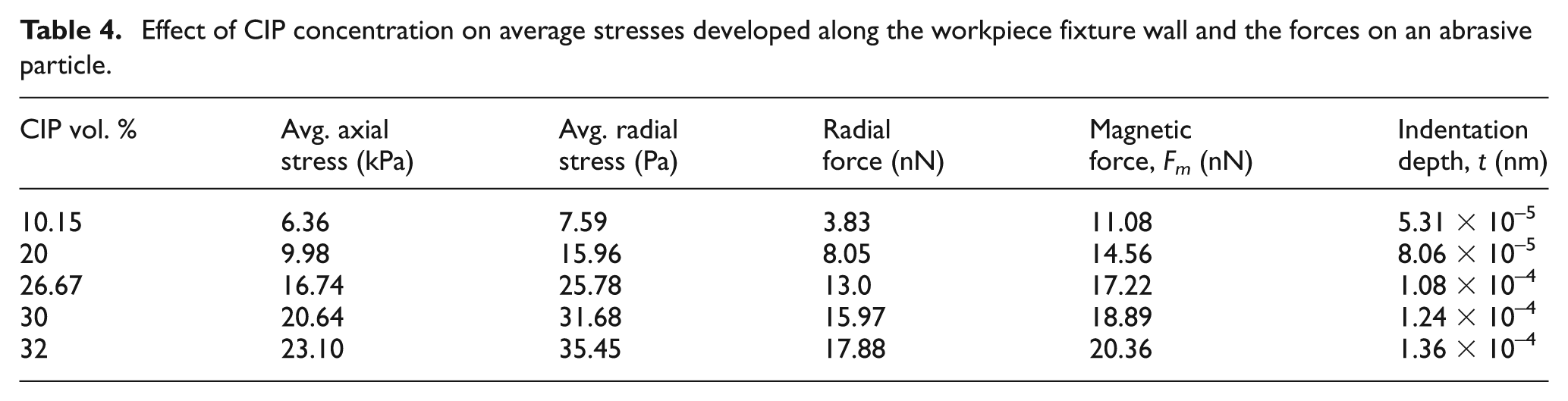
With the rheological data provided in Table 3, the MRP fluid is simulated for different CIP concentrations in the computational domain. The radial variation of the axial velocity profiles at the (a) inlet, and (b) outlet of the finishing Zone (Zone II) are shown in Figure 11(a) and (b), respectively. The area weighted average axial and radial stresses at different CIP concentrations are tabulated in Table 4. It can be seen that with the increase in CIP concentration, inlet and outlet velocity reduces (Figure 11(a) and (b)) and the axial and radial stresses increase (Table 4). The reason for such behaviour is as follows.
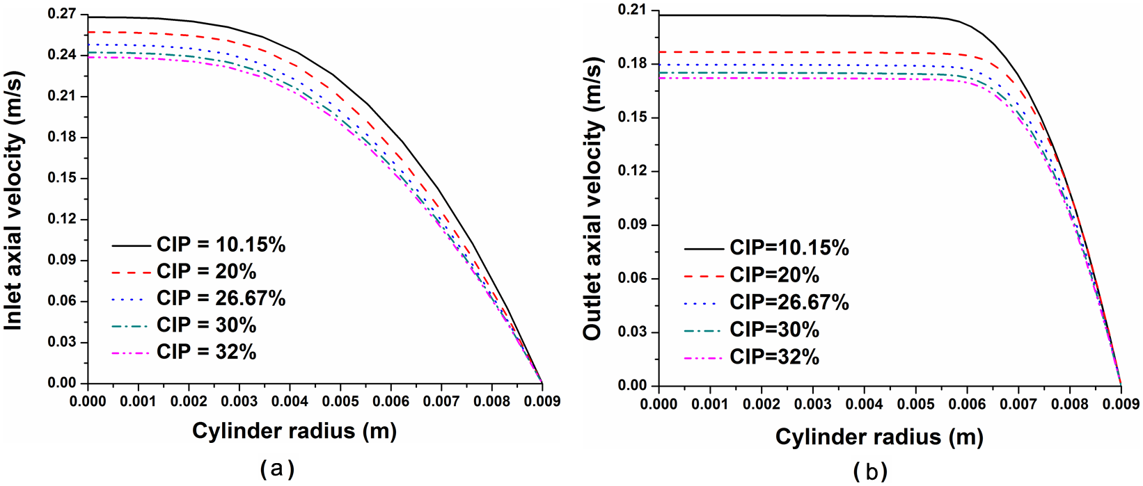
Radial variation of axial velocity profiles: (a) at the entry and, (b) exit of the finishing Zone (Zone II) at different CIP concentrations (SiC = 10%, grease = 12%, rest of the fluid is paraffin oil). Finishing conditions: 37.5 bar pr, 700 finishing cycles with N17 permanent magnet.
Effect of CIP concentration on average stresses developed along the workpiece fixture wall and the forces on an abrasive particle.
CIP is the main ingredient of the MRP fluid composition, and gives a significant contribution to the rheological properties of the MRP fluid. From Table 3, it is found that a higher concentration of CIPs increases yield stress and viscosity of the polishing medium significantly and the simulated magnetic field at the workpiece surface is also increased marginally. Off-state yield stress and viscosity of the polishing medium also increase to some extent (Table 3). Hence, the axial velocity at the inlet (Figure 11(a)) and outlet (Figure 11(b)) in the finishing zone (Zone II) reduces with the increased CIP concentration. Also, at a higher volume fraction, a highly compact BCT structure of particles could be expected, where the restriction of affine deformation leads to a larger yield stress. 10 For the same reason the polishing medium generates higher axial and radial stresses along the workpiece fixture wall at higher CIP concentration (Table 4).
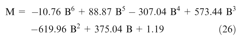
The magnetization (M) plots, as a function of applied magnetic field (B), are shown in Figure 12(a) at different CIP concentrations. From this figure, it is observed that the hysteresis of the MRP fluids is low and exhibits low levels of magnetic coercivity, which will lead to negligible remnant magnetization in the MRP fluid. This may play an important role in the long-term redispersibility of the polishing medium. From Figure 12(a), it is also observed that, with the increase in the concentration of CIPs in the MRP medium, the saturation magnetization becomes larger owing to denser clustering of the CIP chains at higher CIP concentrations for the same magnetic field. The data plotted at the first quadrant of the curve in Figure 12(a) are best fitted (with co-efficient of multiple determination, R2 = 0.99) with a polynomial equation and is given in equation (26) for 10.15% CIPs
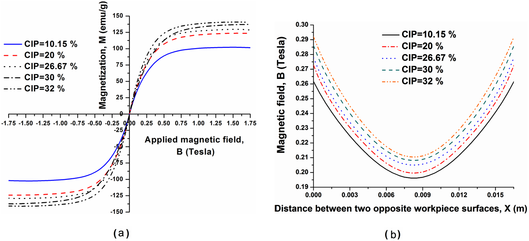
(a) Magnetization (M) versus magnetic field (B) relationship of the MRP fluid, (b) variation in simulated magnetic field (B) with a change in distance (X) between two opposite flat workpiece surfaces of N17 permanent magnet at different CIP concentrations.
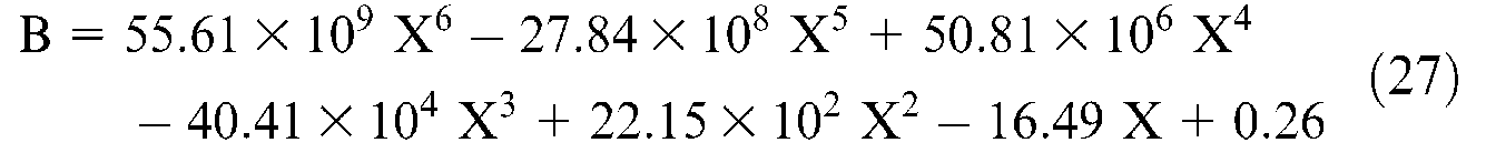
The simulated magnetic field, B (Tesla) of the MRP fluid at different CIP concentrations is plotted in Figure 12(b) as a function of distance, X (m) in between two workpieces. From Figure 12(b), it is observed that, with the increase in the CIP concentration in the polishing medium, the simulated magnetic field at the workpiece surface increases owing to the increased MR effect at higher CIP concentrations. These data are best fitted (R2 = 0.99) with a polynomial equation (equation (27)) for 10.15% CIPs
Similarly, at other CIP concentrations, the data shown in Figure 12 are fitted but not shown here owing to space constraint. Table 4 shows the radial and magnetic force on a single abrasive particle and indentation depth on the workpiece surface at different CIP concentrations.
Figure 13(a) shows the experimental and simulated surface roughness plots with different CIP concentrations. From this figure, it can be seen that the simulated and experimental final surface roughness values almost match each other with different CIP concentrations with a maximum difference of 0.02 μm between them. From Figure 12(b), it is observed that, with an increase in the CIP concentration, the magnetic field at the workpiece surface increases. At higher CIP concentrations, CIPs in the MRP fluid form a thick column of chains holding abrasive particles in between the chains and within the chains with higher force leading to higher indentation force on the active abrasives. Also, with the increase in the CIP concentration, axial and radial stresses along the workpiece surface increase (Table 4), which creates a higher indentation on the workpiece surface. As the MR effect increases with higher CIP concentration, surface finish also improves.
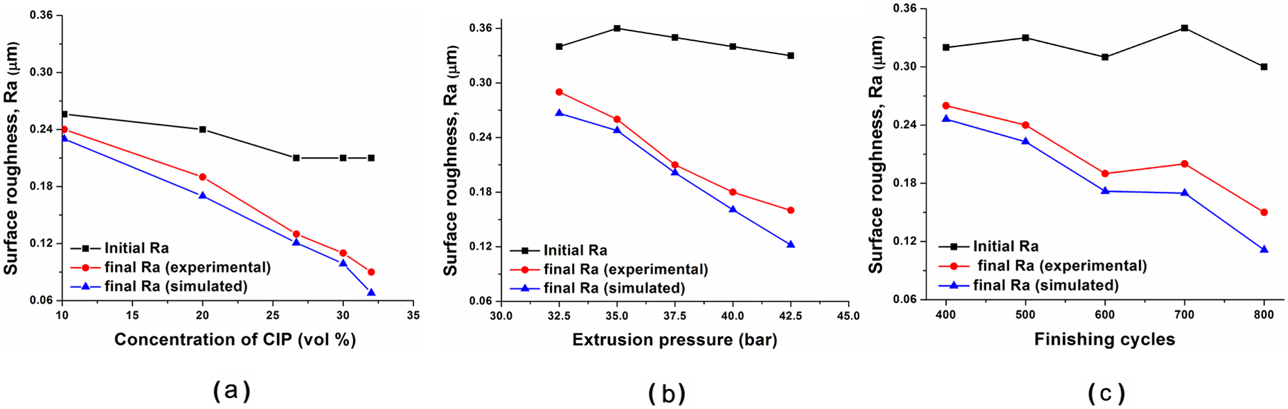
Comparison of simulated and experimental surface roughness values with different (a) CIP concentrations, (b) extrusion pressures, and (c) finishing cycles.
From Figure 13(a), it has also been found that the simulated final surface roughness values are lower than the corresponding experimental results for all the cases considered here. During simulation, it has been assumed that all the abrasive particles touching the workpiece surface are active and an equal amount of material is removed by each one of them in each finishing cycle. During the actual finishing operation, it does not happen. Hence the deviation between the simulated and experimental results exists. The wear of the abrasive cutting edges is not considered during simulation. Further, the simulated results give a better Ra value owing to the assumption that the MRP medium is in a static state, although the polishing medium itself gets sheared during finishing.
Figure 14 shows (a) the initial roughness profile, (b) the final simulated profile, and (c) the measured surface roughness profiles for 32% CIP concentrations. From Figure 14, it is observed that the final (b) simulated, and (c) measured surface roughness profiles match well. The rest of the surface roughness profiles at different CIP concentrations are not provided here owing to space limitations. It is found that, with the increase in CIP concentrations, the surface roughness profile becomes smoother owing to the increased depth of indentation at higher CIP concentrations, which leads to better finishing performance.
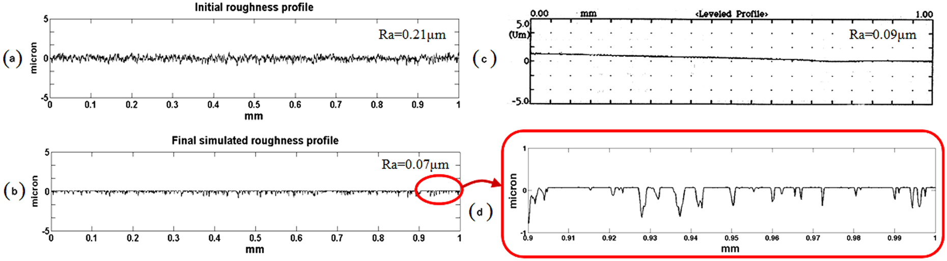
(a) Initial profile, (b) final simulated profile, and (c) measured final surface roughness profile for 32% CIP concentration; (d) magnified view of the simulated surface roughness profile for the marked portion of the curve in (b).
As observed in Table 4, the axial stress is much higher than the radial stress of the fluid inside the workpiece fixture and the width of the valleys along the mean line is less than the size of the abrasive. Therefore, the abrasive particles cut the roughness peaks along a straight line at each finishing cycle and the same is reflected in both measured (Figure 14(c)) and simulated (Figure 14(b)) surface roughness profiles. The magnified view of the simulated surface roughness profile for the marked portion of the curve in Figure 14(b) is shown in Figure 14(d) where the straight line cut of the abrasive particle on the roughness profile is clearly shown.
Effect of extrusion pressure
To study the effect of extrusion pressure on surface finish, five numerical finishing experiments were conducted at different pressures (Table 5) with N48 permanent magnet. The evaluated inlet velocity in Zone I at different pressures is given in Table 5. Using the above information, the polishing medium is simulated at different extrusion pressures.
Effect of extrusion pressure on average stresses developed along the workpiece fixture wall and the forces on an abrasive particle.
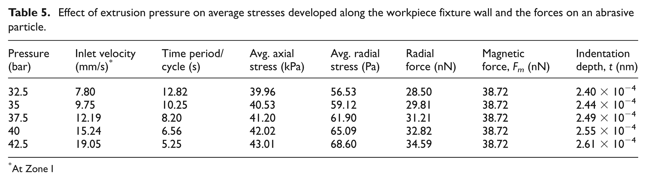
At Zone I
The simulated axial velocity profiles at the (a) entry, and (b) exit of Zone II are given in Figures 15(a) and (b), respectively, at different extrusion pressures. In Figure 15(b), the flat portion of the velocity profile, where the velocity gradient ≈ 0, is called the solid core or plug flow region and beyond that there is a sharp change in the velocity gradient near the wall. With the increase in the extrusion pressure from 32.5 to 42.5 bar, the plug flow radius of the velocity profile decreases for a fixed magnetic field (Figure 15(b)). The radial variation of the shear stress (
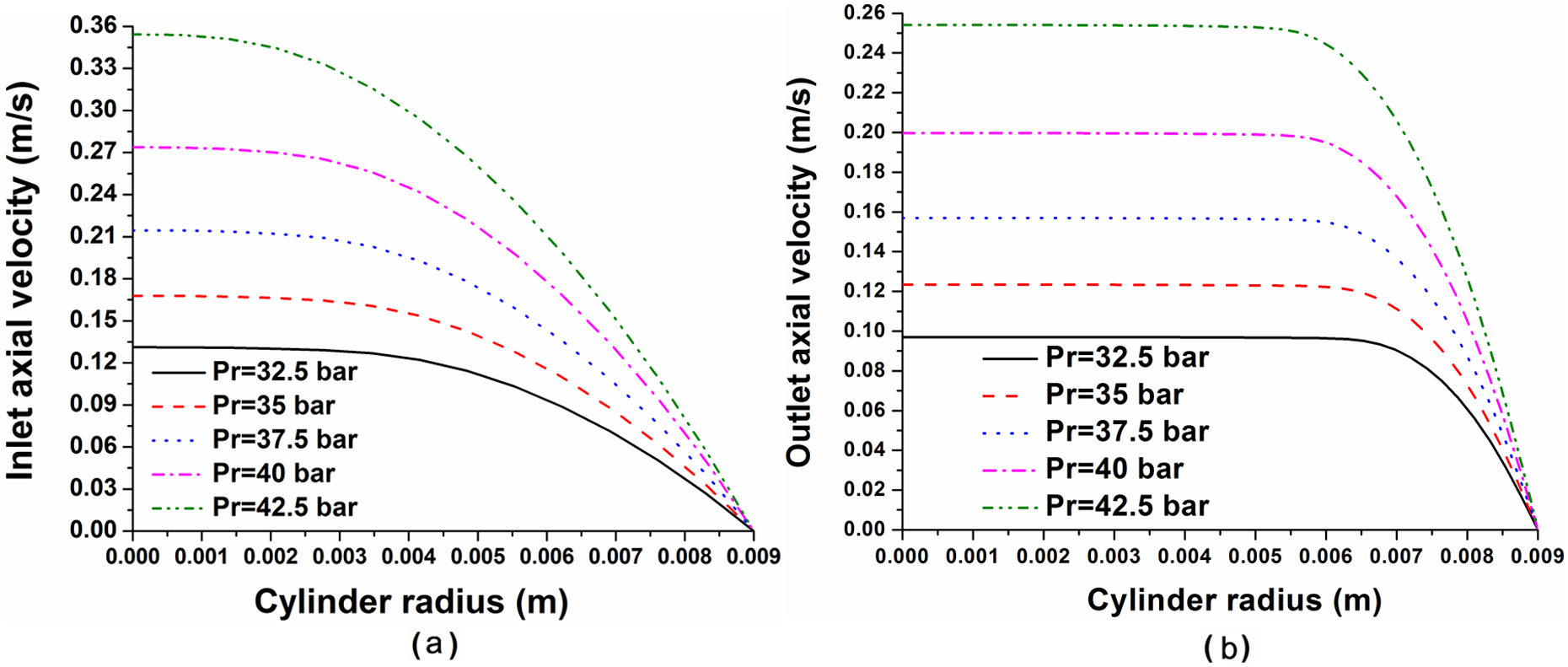
Radial variation of axial velocity profiles at the (a) inlet, and (b) outlet of the finishing zone (Zone II) at different extrusion pressures (26.67% CIP, 13.33% SiC). Finishing conditions: 700 finishing cycles with N48 permanent magnet (Zone I:

Yielding of the fluid occurs at the solid core radius,
Similarly, as in Figure 12(a) and (b), magnetization M (emu/g) of the MRP fluid with different magnetic fields, B (Tesla) and simulated magnetic fields, B (Tesla) as a function of distance, X (m) in between two workpieces in front of two opposite poles of the permanent magnet, are plotted and the best fitted polynomial equations (R2 = 0.99) of the data are given in equations (28) and (29), respectively
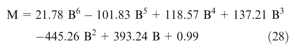
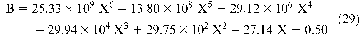
Table 5 shows the radial and magnetic force on a single abrasive particle and the indentation depth on the workpiece surface at different extrusion pressures.
The simulated and experimental surface roughness results at different extrusion pressures are shown in Figure 13(b). The theoretically calculated Ra values are in close agreement with the experimental results except at a higher extrusion pressure. At the higher extrusion pressure, owing to the shear thinning nature of the polishing medium, the strength of the fluid reduces. 4 Hence, the experimental final surface roughness value is higher than the simulated one at the higher extrusion pressure.
Effect of finishing cycles
For evaluating the effect of the number of finishing cycles on the finishing performance, the finishing cycles are varied from 400 to 800 with an interval of 100 cycles. As the polishing is performed under the same experimental conditions (except finishing cycles) with the same polishing medium as in the section ‘Effect of extrusion pressure’, the output results provided in Table 5 at 37.5 bar pressure are utilized for the simulation of surface roughness for the current case. The time period for the single finishing cycle is 8.20 s.
Figure 13(c) shows a comparison between the experimental and simulated surface roughness values at different finishing cycles. From this figure, it is observed that the surface finish is improved with the increase in the number of finishing cycles for both cases. Comparatively, a larger difference in final surface roughness values between the experimental and simulated results is observed beyond 600 finishing cycles. The final surface roughness value decreases rapidly for the initial finishing cycles during finishing owing to the smooth removal of the roughness peaks. However, at higher finishing cycles, the shear area of the roughness peaks increases, which requires a higher cutting force leading to less reduction in the roughness value experimentally. However, the assumption of constant indentation to the roughness peaks at each finishing cycle leads to a constant finishing rate in the simulated results. Hence, the differences in the final surface roughness values between the simulated and experimental results are observed beyond 600 finishing cycles.
Conclusions
On the basis of the present work reported in this article, the following conclusions are drawn.
A CFD simulation of the flow of the MRP medium inside the cylindrical workpiece fixture is performed to calculate the axial and radial stresses developed on the fixture wall. The axial velocity profiles of the simulation results match well with the analytical solution of the Bingham plastic pipe flow equation. It is observed from the numerical simulation that a higher axial pressure gives rise to a smaller plug flow region at a given magnetic field.
From the velocity vector plot of the MRP fluid in the finishing zone, it is observed that the velocity vectors are slightly inclined towards the wall near the inlet section, which helps the abrasive particles in the polishing medium to efficiently scoop up the surface asperities from the workpiece surface.
From comparison of the magnetic fields between the Maxwell simulation results with experimentally measured magnetic fields without the polishing medium, it is found that they are in good agreement.
From the analysis of forces acting on the abrasive particles, it has been found that the axial force on an active abrasive particle is greater than the material reaction force, which establishes the shearing action of the abrasive particle on the workpiece surface during finishing.
The final surface roughness value predicted from the simulation results of the stainless steel workpiece are lower than the corresponding experimental results for all the cases considered here, although there is insignificant difference between them.
The simulated final surface roughness profile matches well with the measured final roughness profile validating the proposed model of the MRAFF process with the process physics and mechanism of the finishing action.
From the simulated final surface roughness profile, it is observed that the abrasive particles cut the roughness peaks along a straight line at each finishing cycle, as the axial stress of the medium is much higher than the radial stress and the width of the valleys along the mean line is lesser than the size of the abrasive.
The surface finish improves with higher CIP concentrations owing to the increased strength of the CIP chain structure at higher CIP concentrations.
Footnotes
Appendix
Acknowledgements
We sincerely thank BASF Germany for making CIPs available at different grades for our research work.
Funding
This work was supported by the Department of Science and Technology, New Delhi [grant number SR/S3/NERC/0072/2008] entitled “Rotational – magnetorheological abrasive flow finishing (R-MRAFF)”.